
Angular Spectral Density and Information Entropy for Eddy Current Distribution

School of Mechanical Engineering, Beijing Institute of Technology, Beijing 100081, China
*
Author to whom correspondence should be addressed.
Entropy 2016, 18(11), 392; https://doi.org/10.3390/e18110392
Submission received: 20 September 2016
/
Revised: 2 November 2016
/
Accepted: 7 November 2016
/
Published: 10 November 2016
(This article belongs to the Special Issue Maximum Entropy and Its Application II)
Abstract
:Here, a new method is proposed to quantitatively evaluate the eddy current distribution induced by different exciting coils of an eddy current probe. Probability of energy allocation of a vector field is modeled via conservation of energy and imitating the wave function in quantum mechanics. The idea of quantization and the principle of circuit sampling is utilized to discretize the space of the vector field. Then, a method to calculate angular spectral density and Shannon information entropy is proposed. Eddy current induced by three different exciting coils is evaluated with this method, and the specific nature of eddy current testing is discussed.
1. Introduction
Improving the performance of eddy current (EC) non-destructive testing (NDT) systems is important for enhancing the accuracy of such measurement devices, and the innovation in EC probes is one of the most important ways to achieve this goal. An EC probe is mainly composed of exciting coils and a pick-up element, and carries a non-uniform current that induces the eddy current in conductive materials. Depending on applications, different pick-up elements, coils, and sensors such as Superconducting Quantum Interference Device (SQUID), Hall, Anisotropic Magnetoresistance (AMR), Giant Magneto-impedance (GMI), Giant Magnetoresistance (GMR) [1,2,3,4,5,6], and Tunnel MagnetoResistance (TMR) [7] are used.
However, depending on the goal, many publications propose the use of different waveforms of exciting current. The conventional EC testing method is based on the single-frequency current exciting waveform and is used in many fields, such as defect detection and stress measurement. Multi-frequency EC testing [8] was proposed to detect defects in different depths, and pulse current exciting current [9] was proposed to enrich the frequency component. Chirp excitation [10], whose frequency changes with time, was used for frequency sweep. In short, the innovations in exciting current waveforms only improved the eddy current distribution over time at a certain position. However, the sensitivity of an EC probe depends on the relationship between the EC direction and the defect direction, so different exciting coils were proposed to improve the eddy current distribution, such as the meandering magnetometer (MWM) [11,12], rosette-like [13], fractal Koch curve [14,15], and rectangular exciting coil. Moreover, a rotating field EC planar probe [2,4,6] was proposed to generate an eddy current that can automatically rotate in the time domain. Thus, eddy current direction both in time and in space domains is of vital importance to a probe’s sensitivity.
To improve the performance of an EC probe, optimizing the eddy current distribution induced by the EC probe is a promising approach. However, the eddy current distribution can only be observed by the eyes and there is no appropriate index to be considered as an objective function. Shannon information entropy measures the uniformity of the distribution of information distribution. In 2016, Zhang et al. [16] first used the Shannon information entropy to evaluate eddy current in a plane distributed in different directions. To improve this method, a theoretical approach is proposed in this paper.
In general, probability density of energy allocation of a multidimensional vector in multidimensional space is modeled via the conservation of energy. Probability density discretization is described in Section 2 and Section 3, describing the discretization method for space utilizing the idea of quantization and sampling from circuit principle. Moreover, in Section 4, the method is applied to EC distribution evaluation, and an angular spectral method is proposed. Section 5 presents the method to calculate information entropy. Section 6 briefly describes the method of eddy current acquisition. In Section 7, the main results are presented and analyzed. Conclusions and future studies are addressed in the last section.
2. Energy of Field Distribution Density of a Multidimensional Vector in a Multidimensional Space
Without loss of generality, a multidimensional vector in a multidimensional space is investigated in this section. In general, a vector field includes two kinds of information: position vector and field vector. Assuming is an m-dimensional space (i.e., the position vector space), vector in represents a point in and is in a position of the position vector space. Similarly, assuming is n-dimensional space (i.e., the field vector space) the vector in represents a field vector in in one position vector. In the position vector space , if m = 0, is a 0-dimensional space, like a point; if m = 2 or 3, is a 2-dimensional planar space and a 3-dimensional cubic space; if m = 4, is a time–space. In the field vector space , if n = 1, is a scalar vector; if n = 2, is a 2-dimensional vector, like the EC vector studied in this paper; if n = 3, is a 3-dimensional electric field, magnetic field or a gradient field for temperature field. Different kinds of fields are distributed in different ways, such as a uniform field and a radial field, among others, so the different field distribution may carry different amounts of information.
Assume the function about position vector and field vector , has the following property
where is the energy allocation at position when the field vector is . For example, in a 2-dimensional EC vector field
is the energy allocation of EC at position , where the EC vector is .
For Equation (1), the total energy of a field in the whole position vector space and the field vector space is
here is the infinitesimal position vector space and is the infinitesimal field vector space. Dividing both sides of Equation (3) gives
Function is defined as
is a percentage of the energy allocation of field at position where the field vector is . By substituting Equation (5) into Equation (4) one obtains
According to Equation (1)
The aforementioned Equations (6) and (7) represent the normalization condition and the non-negative condition, respectively and is additive. Thus, is defined as a probability density of field energy allocation at position where the field vector is .
By ignoring information of and only considering the position of field energy allocation, marginal probability density
represents the probability of field energy allocation at position .
Similarly, by ignoring the information of position and only considering the vector of field energy allocation, marginal probability density
represents the probability of field energy allocation for anywhere when the field vector is .
Certainly, if the same component of vectors and is only considered, types of marginal probability densities exist, each of which has their own obvious physical meaning.
The probability density function in this study is modeled by imitating the wave function of quantum mechanics. In quantum mechanics [17], the wave function obeys the superposition of the principle to explain the phenomenon of interference, diffraction and others; however is considered as a probability. Similarly, the eddy current distribution vector induced by different coils obeys the superposition principle. For example, , and are eddy current density distributions induced by two different coils, and is the eventual eddy current distribution. Due to and , is selected to model the probability density function.
3. Probability Density Discretization
To calculate the information entropy of the field, probability density described in Section 1 must be discretized. Borrowing the idea of an analog-to-digital converter (ADC) in circuit principle, the position vector space and the field vector space are discretized by equal interval sampling. Thus, the continuous spaces and are converted to discretized spaces. The combination of one point in the discretized position vector space and one point in the discretized field vector space is defined as a discrete random variable. All discrete random variables form the probability density of space. Thus, the probability of the discretized random variable is
here , is the probability of event () and the energy allocation percentage of the field at position when the field vector is . Similar to Equation (5) in Section 1, is the normalization condition, non-negative and additive.
Similar to Section 1, is a joint probability density function for the m + n dimensional discrete random variable. has types of marginal probability density functions. If the information of field vector is ignored and the position of field energy allocation is only considered, a marginal probability density of the discrete random variable is given by
here, is called space spectral density.
Similarly, by ignoring the information of position and only considering the vector of field energy allocation, a marginal probability density of the discrete random variable is expressed as
here, is called gesture spectral density.
4. Information Entropy of Energy Allocation of a Vector Field
Shannon information entropy is the expected value of self-information of a discrete random variable. In this study, information entropy of energy allocation of a vector field in the whole position vector space and the whole field vector field space is defined as
where is the self-information for event , the base of the logarithmic function is 2 in this study. The physical meaning of is the following: if the probability of event is strong, the event is more decided, so the self-information of event is small, and vice versa; if the probability of event equals 1, the event is absolutely certain, so its self-information is 0.
If the information entropy in position vector space is only considered, the special entropy is defined as
Similarly, if the information entropy in the field vector space is only considered, the special entropy is defined as
Certainly, information entropy of other marginal probability densities can be calculated. For example,
where is the information entropy of the field vector space at the particular position .
5. Two-Dimensional EC Vector in a Two-Dimensional Plane
In EC non-destructive testing, the direction of EC vector distribution is very important because it is related to the sensitivity of the probe. In this study, the information entropy of the 2-dimensional EC in a 2-dimensional plane induced by three different exciting coils is calculated and analyzed.
The EC and defect interaction domain is considered as , the 2D field vector space in Cartesian coordinates is , and the 2D field vector space in polar coordinates is .
According to Equation (1), EC energy allocation at where the EC is is defined as
However, EC energy allocation at where the EC in polar coordinates is is defined as
According to the law of conservation of energy
Dividing both sides of Equation (19) by results in
Probability density function of the field can be defined as
Equations (22) and (23) express the non-negativity condition of two kinds of the probability density functions and .
According to Equations (17) and (18), and are complete:
In this study, marginal probability densities and are studied first; and are defined as angular spectral density and angular spectral density along the x-axis, respectively. represents the EC’s energy of the whole space allocated in different directions. However, is the energy of EC at position allocated in different directions. Then, the information entropy and of and are studied.
6. Acquisition of EC Vector
According to [16], three finite element models were studied and their EC distributions were acquired. The studied exciting coils were a line, a circle, and a second-order Koch curve, respectively, the centers of which were all located in the origin of coordinates and the line was along the y-axis. The eddy current in a hypothetical defect-eddy current interaction domain was sampled at equal intervals. The interaction domain, shown in Figure 1, was a rectangle with axial symmetry along both the x-axis and y-axis. For all cases and the x-axis were sampled with 0.5 mm-long steps. However, different values were chosen to simulate different lengths of defects. In the y direction, EC sampling was of 64 points uniformly distributed within . Angle and magnitude of eddy current were calculated by
where and are the component and component of the EC vector at position , respectively; and are the angle to the x-axis and magnitude of the EC vector at position .
7. Results and Discussion
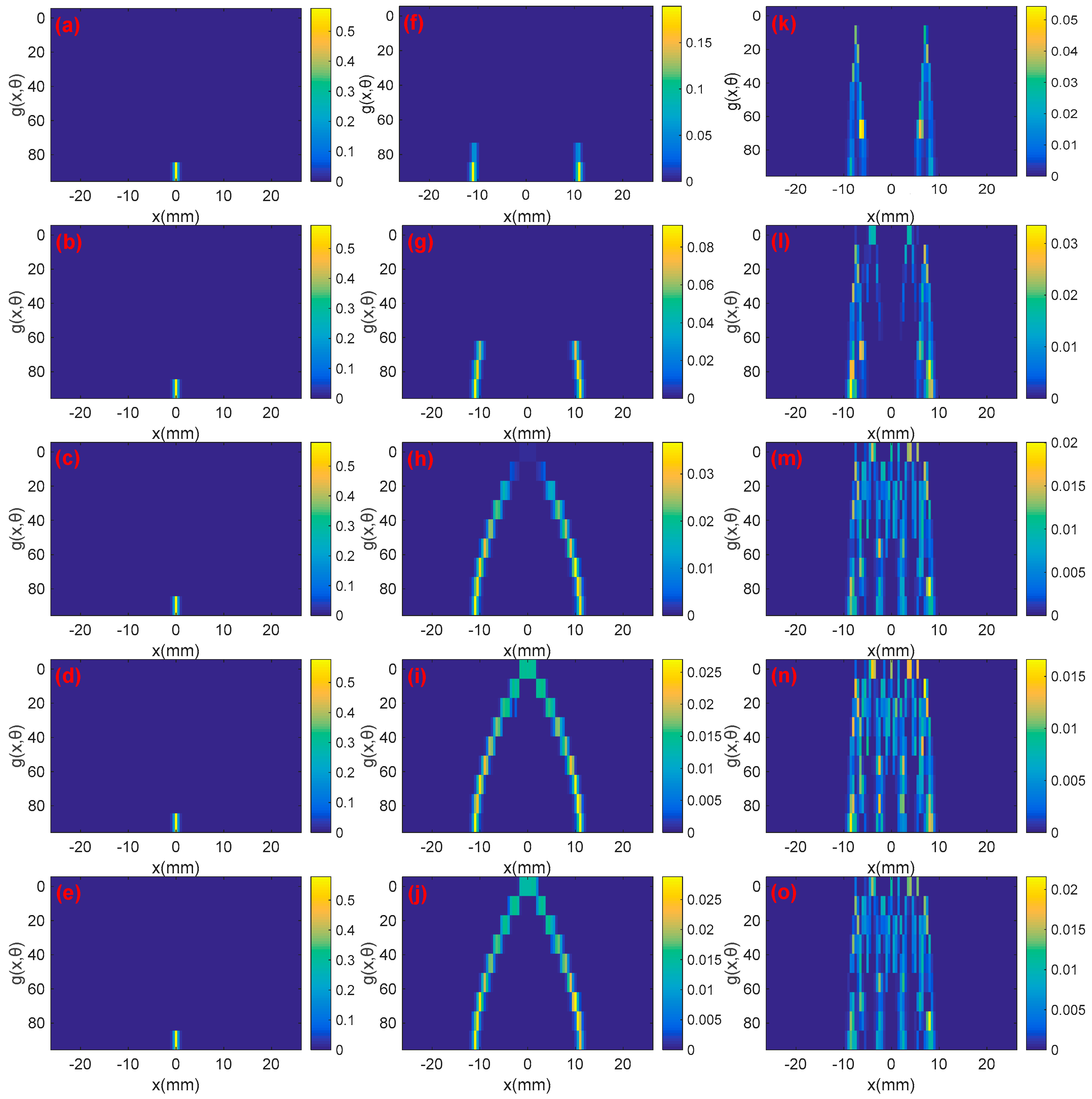
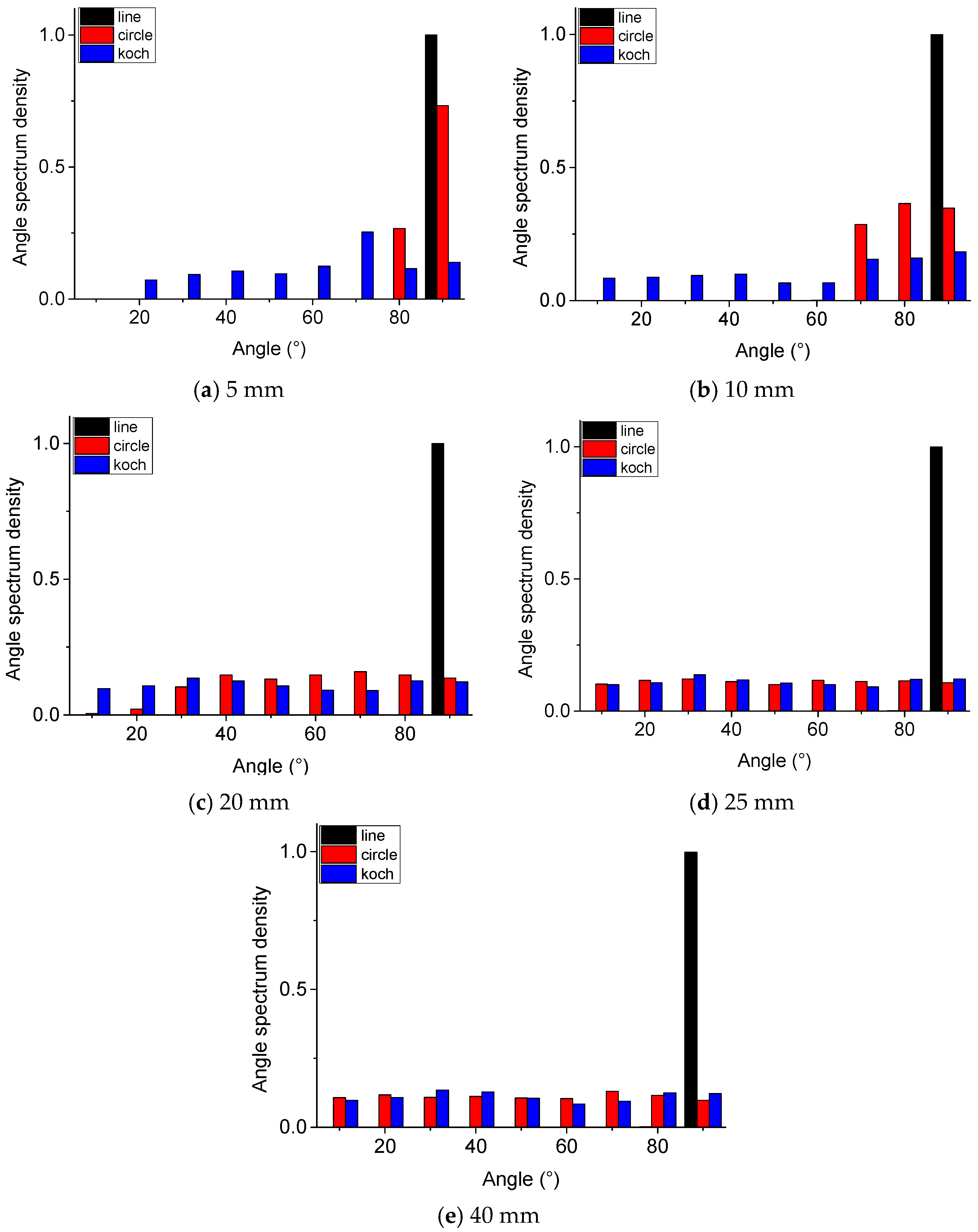
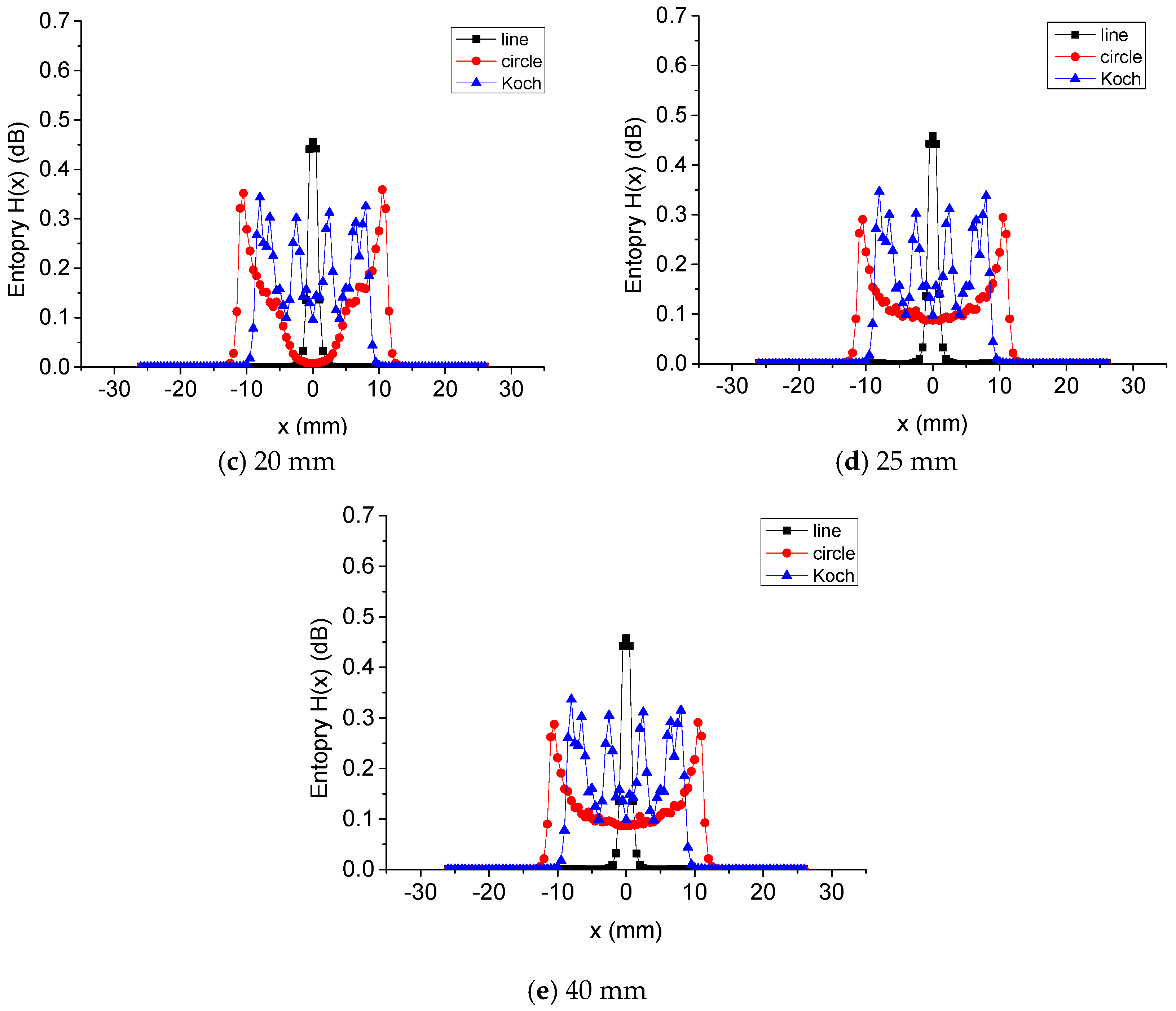
Angular spectral densities along the x-axis of the EC distribution induced by different exciting coils of different widths of the interaction domain are shown in Figure 2. Angular spectral densities are shown in Figure 3. Information entropy and are shown in Figure 4 and Figure 5, respectively.
7.1. Analysis of Angular Spectral Density along the x-Axis
The exciting coils and the width of the interaction domain influence the analysis of angular spectral density along the x-axis. As detailed in Figure 2a–e, angular spectral densities along the x-axis of the EC induced by a linear inducer in different width interaction domains are centrally concentrated on 90°.
For a circular exciting coil, the distribution of angular spectral density along the x-axis is shown in Figure 2f–j. As the interaction domain width increases, angular spectrum density along the x-axis distributes to different angles. When the width of the interaction is 5 mm, the angular spectral density along the x-axis is only distributed to 90°, but at 25 mm or 40 mm, the eddy current density ranges from 0° to 90° angles. Note that the angular spectrum is concentrated in a narrow angle at a certain x because the EC induced by one winding is distributed on the position underneath the coil.
For the Koch exciting coil, differences in angular spectrum density along the x-axis can be seen in Figure 2k–o: angular spectral density along the x-axis ranges from 0° to 90°, and at a certain value x, it is located in a large angle range. For linear and circular exciting coils, it is distributed on a certain angle at a certain x.
7.2. Angular Spectral Density
As shown in Figure 3, angular spectral density represents the EC distribution in different angles on the whole interaction domain. Similar to the cases described in Section 7.1, the angular spectral density for linear exciting coils is distributed in a narrow range. For a circular coil, its range increases with the width of the interaction domain. For a Koch coil, when the width of the interaction is 5 mm, angular spectral density ranges from 30° to 90°. However, when the widths of the interaction are larger than 10 mm, the density is distributed in all angles, and the larger the width, the more uniform the angular spectral density. In summary, when the interaction width is smaller, the angular spectral density of a circular coil is similar to that of the linear coil shown in Figure 3a. However, when the interaction width is larger, the angular spectral density is similar to that of a Koch coil, shown in Figure 3b.
7.3. Information Entropy along the x-Axis
The information entropy for the EC distributed in different angles along the x-axis is shown in Figure 4. For linear exciting coils, has only one peak and the peak value remains almost constant with the increasing width of the interaction domain.
For a circular coil, has two peaks. As the width of the interaction domain increases, the peak value decreases but the value of between the two peaks increases.
For Koch coils, the number and the position of the peaks of change with the width of the interaction domain. The peak value decreases with the increasing of the width of the interaction domain, but the value between the peaks also increases.
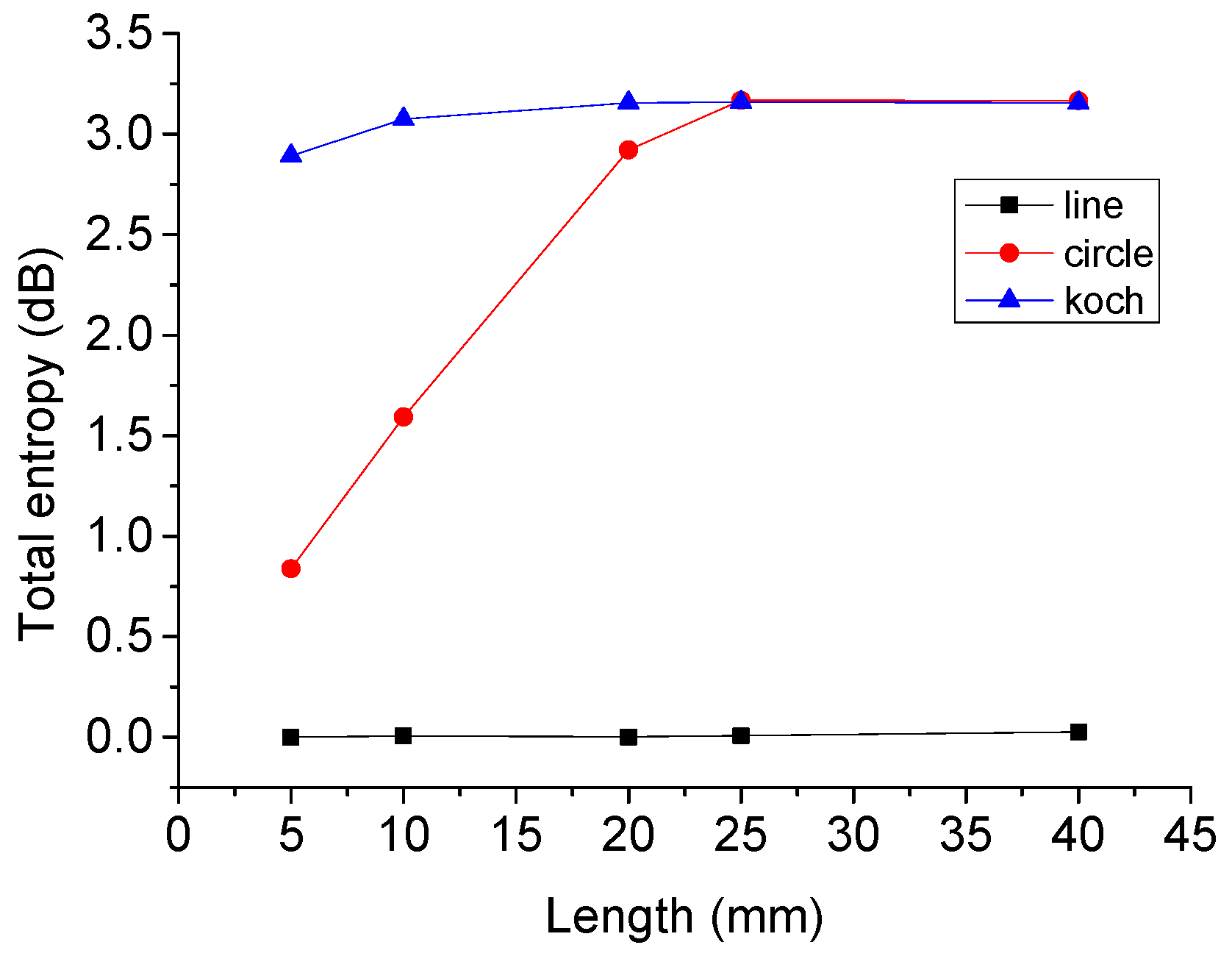
7.4. Information Entropy of the Whole Interaction Domain
The information entropy of the whole interaction domain is shown in Figure 5, measuring the complexity of the EC distribution at different angles. For the EC induced by a linear coil, its information entropy for different widths of interaction domains is nearly zero. Angular spectrum density for linear exciting coils is concentrated in a narrow angle range, so . In this case, the EC is a high-certainty event, and its self-information is almost zero .
For other exciting coils, when the width of the interaction domain is larger than 25 mm, the entropy of the circular and Koch coils approaches its maximum value of 3.1699. In this case, the interaction domain covers the whole exciting coil, and the angular spectral density is almost uniformly distributed; therefore, the information entropy reaches its maximum value . When the width of the interaction domain is smaller than 25 mm, the total information entropy of the EC distributed in more than one angle increases with the width of the interaction domain. However, the rate of change of the information entropy of the Koch coil is larger than that of the circular coil. Therefore, when the width of interaction is 5 mm, the total information entropy of the Koch coil is more than three times higher than that of the circular coil. This validates the idea of using a Koch exciting coil as its induced EC is allocated in a larger angle range of a smaller domain compared to circular and linear exciting coils.
8. Conclusions
Without loss of generality, energy allocation density of a multi-dimensional vector field in a multidimensional space is proposed using conservation of energy. Via the method of quantization and sampling from circuit theory, the position vector space and field vector space are discretized. Then, the quantity of information of the field, using information entropy, is proposed. Finally, the proposed method is applied to evaluate two-dimensional eddy currents in a plane. Angular spectral density is proposed to illustrate the EC allocated in different directions, and the complexity of EC distribution in different directions is calculated by using information entropy. The EC induced by three typical exciting coils, i.e., linear, circular and Koch, is evaluated. Results highlight that angular spectral and information entropy can intrinsically and quantitatively reveal the disturbance principle of EC NDT.
In the next study, the EC in time–space, induced by the rotating field EC method and pulse EC testing method will be evaluated and analyzed.
Acknowledgments
This work was financially supported by the National Nature Science Foundation of China (51275048).
Author Contributions
Guolong Chen conceived and designed the experiments, analyzed the data, contributed reagents/materials/analysis tools and wrote the paper. Weimin Zhang guided the work. Both authors have read and approved the final manuscript.
Conflicts of Interest
The authors declare no conflict of interest.
References
- Yang, G.; Dib, G.; Udpa, L.; Tamburrino, A.; Udpa, S.S. Rotating field EC-GMR sensor for crack detection at fastener site in layered structures. IEEE Sens. J. 2015, 15, 463–470. [Google Scholar] [CrossRef]
- Ye, C.; Huang, Y.; Udpa, L.; Udpa, S.S. Novel Rotating Current Probe With GMR Array Sensors for Steam Generate Tube Inspection. IEEE Sens. J. 2016, 16, 4995–5002. [Google Scholar] [CrossRef]
- Jarvis, R.; Cawley, P.; Nagy, P.B. Current deflection NDE for the inspection and monitoring of pipes. NDT E Int. 2016, 81, 46–59. [Google Scholar]
- Ye, C.; Huang, Y.; Udpa, L.; Udpa, S.; Tamburrino, A. Magnetoresistive sensor with magnetic balance measurement for inspection of defects under magnetically permeable fasteners. IEEE Sens. J. 2016, 16, 2331–2338. [Google Scholar] [CrossRef]
- Sakthivel, M.; George, B.; Sivaprakasam, M. A Novel GMR-Based Eddy Current Sensing Probe with Extended Sensing Range. IEEE Trans. Magn. 2016, 52. [Google Scholar] [CrossRef]
- Ye, C.; Huang, Y.; Udpa, L.; Udpa, S.S. Differential Sensor Measurement with Rotating Current Excitation for Evaluating Multilayer Structures. IEEE Sens. J. 2016, 16, 782–789. [Google Scholar] [CrossRef]
- Jander, A.; Smith, C.; Schneider, R. Magnetoresistive sensors for nondestructive evaluation. In Proceedings of the SPIE 5770, Advanced Sensor Technologies for Nondestructive Evaluation and Structural Health Monitoring, San Diego, CA, USA, 13 May 2005; pp. 1–13.
- Bernieri, A.; Betta, G.; Ferrigno, L.; Laracca, M. Crack Depth Estimation by Using a Multi-Frequency ECT Method. IEEE Trans. Instrum. Meas. 2013, 62, 544–552. [Google Scholar] [CrossRef]
- Buck, J.; Underhill, P.; Mokros, S.; Morelli, J.; Babbar, V.; Lepine, B.; Renaud, J.; Krause, T.W. Pulsed eddy current inspection of support structures in steam generators. IEEE Sens. J. 2015, 15, 4305–4312. [Google Scholar] [CrossRef]
- Betta, G.; Ferrigno, L.; Laracca, M.; Burrascano, P.; Ricci, M.; Silipigni, G. An experimental comparison of multi-frequency and chirp excitations for eddy current testing on thin defects. Measurement 2015, 63, 207–220. [Google Scholar] [CrossRef]
- Zilberstein, V.; Grundy, D.; Weiss, V.; Goldfine, N.; Abramovici, E.; Newman, J.; Yentzer, T. Early detection and monitoring of fatigue in high strength steels with MWM-arrays. Int. J. Fatigue 2005, 27, 1644–1652. [Google Scholar] [CrossRef]
- Russell, R.; Jablonski, K.D.D.; Washabaugh, A.; Sheiretov, Y.; Martin, M.C.; Golffine, N. Development of Meandering Winding Magnetometer (MWM®) Eddy Current Sensors for the Health Monitoring, Modeling and Damage Detection of High Temperature Composite Materials. Available online: https://ntrs.nasa.gov/search.jsp?R=20120004241 (accessed on 8 November 2016).
- Li, P.; Cheng, L.; He, Y.; Jiao, S.; Du, J.; Ding, H.; Gao, J. Sensitivity boost of rosette eddy current array sensor for quantitative monitoring crack. Sens. Actuators A Phys. 2016, 246, 129–139. [Google Scholar] [CrossRef]
- Chen, G.; Zhang, W.; Qin, F.; Guo, Y. An Eddy Current Probe Based on the Fractal Koch Curve Exciting for Detecting Crack in Metal. Available online: http://www.paper.edu.cn/html/releasepaper/2015/03/428/ (accessed on 8 November 2016). (In Chinese)
- Chen, G.; Zhang, W.; Pang, W.; Qin, F.; Guo, Y.; Wang, C. Analysis on the Working Principle of Eddy Current Probe Using the Koch Curve Exciting Coils. Chin. J. Sens. Actuators 2015, 28, 1454–1458. (In Chinese) [Google Scholar]
- Zhang, W.; Chen, G.; Pang, W. Shannon information entropy of eddy current density distribution. Nondestructive Testing and Evaluation. Nondestruct. Test. Eval. 2016, 1–14. [Google Scholar] [CrossRef]
- Feynman, R.P.; Albert, R.H.; Daniel, F.S. Quantum Mechanics and Path Integrals; Dover: Mineola, NY, USA, 2005. [Google Scholar]
Figure 1.
Defect eddy current (EC) interaction domain.
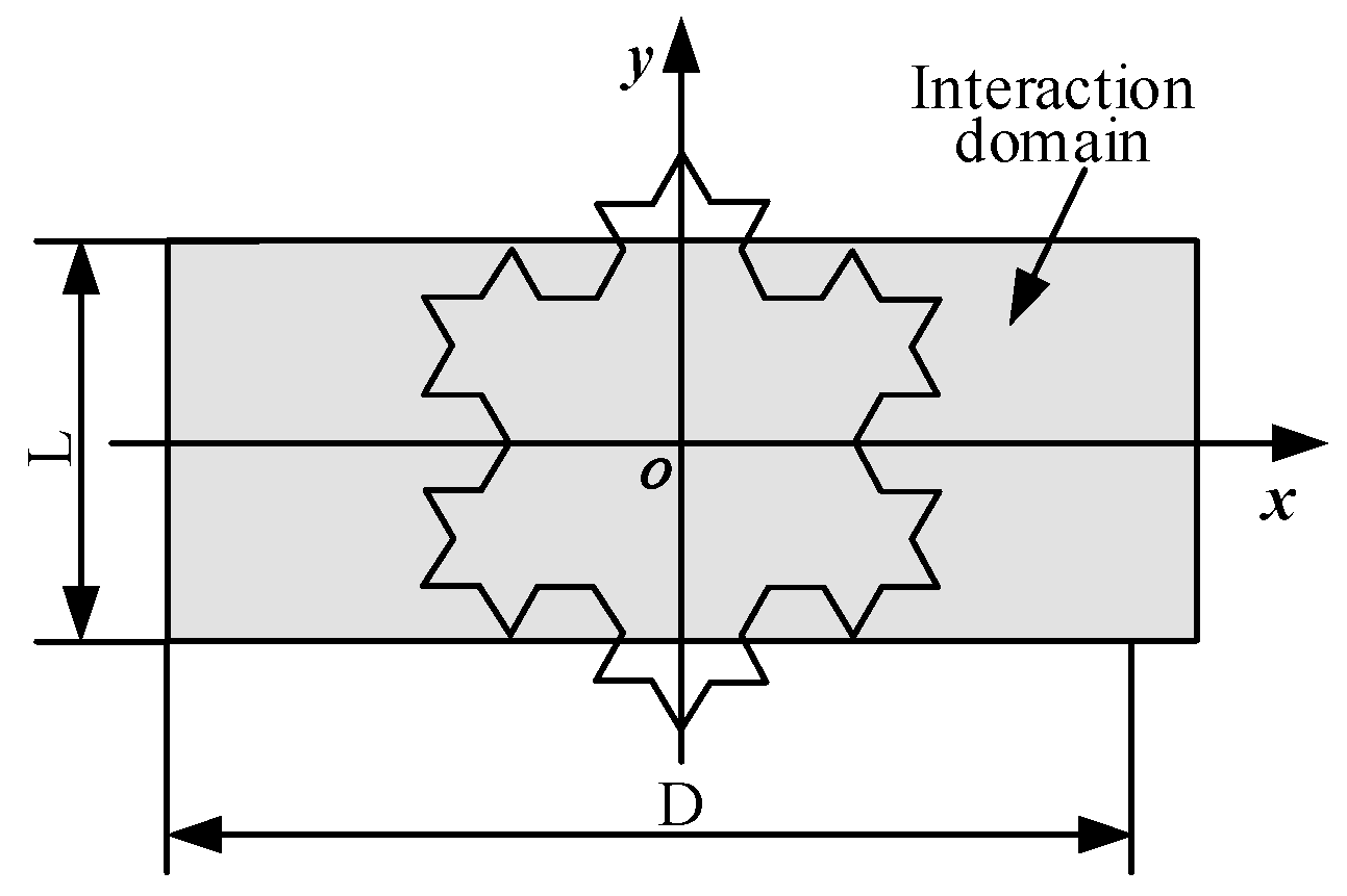
Figure 2.
Angle spectrum density along the x-axis of different exciting coils and different widths of the interaction domain: (a) line exciting, ; (b) line exciting, ; (c) line exciting, ; (d) line exciting, ; (e) circle exciting, ; (f) circle exciting, ; (g) circle exciting, ; (h) circle exciting, ; (i) circle exciting, ; (j) circle exciting, ; (k) Koch exciting, ; (l) Koch exciting, ; (m) Koch exciting, ; (n) Koch exciting, ; (o) Koch exciting, .

Figure 3.
Total angle spectrum for different exciting coils and different widths of the interaction domain. (a) ; (b) ; (c) ; (d) ; (e) .
Figure 3.
Total angle spectrum for different exciting coils and different widths of the interaction domain. (a) ; (b) ; (c) ; (d) ; (e) .

Figure 4.
Information entropy for different exciting coils and different widths of the interaction domain. (a) ; (b) ; (c) ; (d) ; (e)
Figure 4.
Information entropy for different exciting coils and different widths of the interaction domain. (a) ; (b) ; (c) ; (d) ; (e)
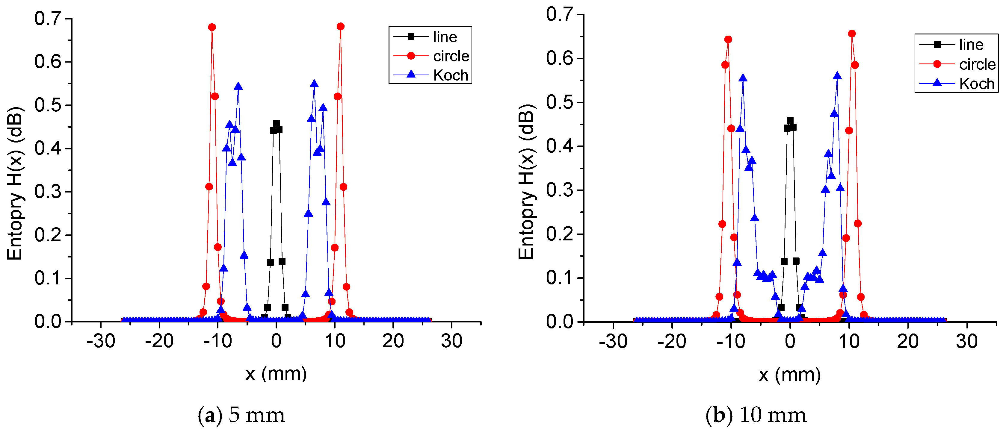

Figure 5.
Total information entropy for different exciting coils and different widths of the interaction domain.
Figure 5.
Total information entropy for different exciting coils and different widths of the interaction domain.
© 2016 by the authors; licensee MDPI, Basel, Switzerland. This article is an open access article distributed under the terms and conditions of the Creative Commons Attribution (CC-BY) license (http://creativecommons.org/licenses/by/4.0/).
Share and Cite
MDPI and ACS Style
Chen, G.; Zhang, W. Angular Spectral Density and Information Entropy for Eddy Current Distribution. Entropy 2016, 18, 392. https://doi.org/10.3390/e18110392
AMA Style
Chen G, Zhang W. Angular Spectral Density and Information Entropy for Eddy Current Distribution. Entropy. 2016; 18(11):392. https://doi.org/10.3390/e18110392
Chicago/Turabian StyleChen, Guolong, and Weimin Zhang. 2016. "Angular Spectral Density and Information Entropy for Eddy Current Distribution" Entropy 18, no. 11: 392. https://doi.org/10.3390/e18110392
Note that from the first issue of 2016, this journal uses article numbers instead of page numbers. See further details here.