
The Geometry of Signal Detection with Applications to Radar Signal Processing


Abstract
:1. Introduction
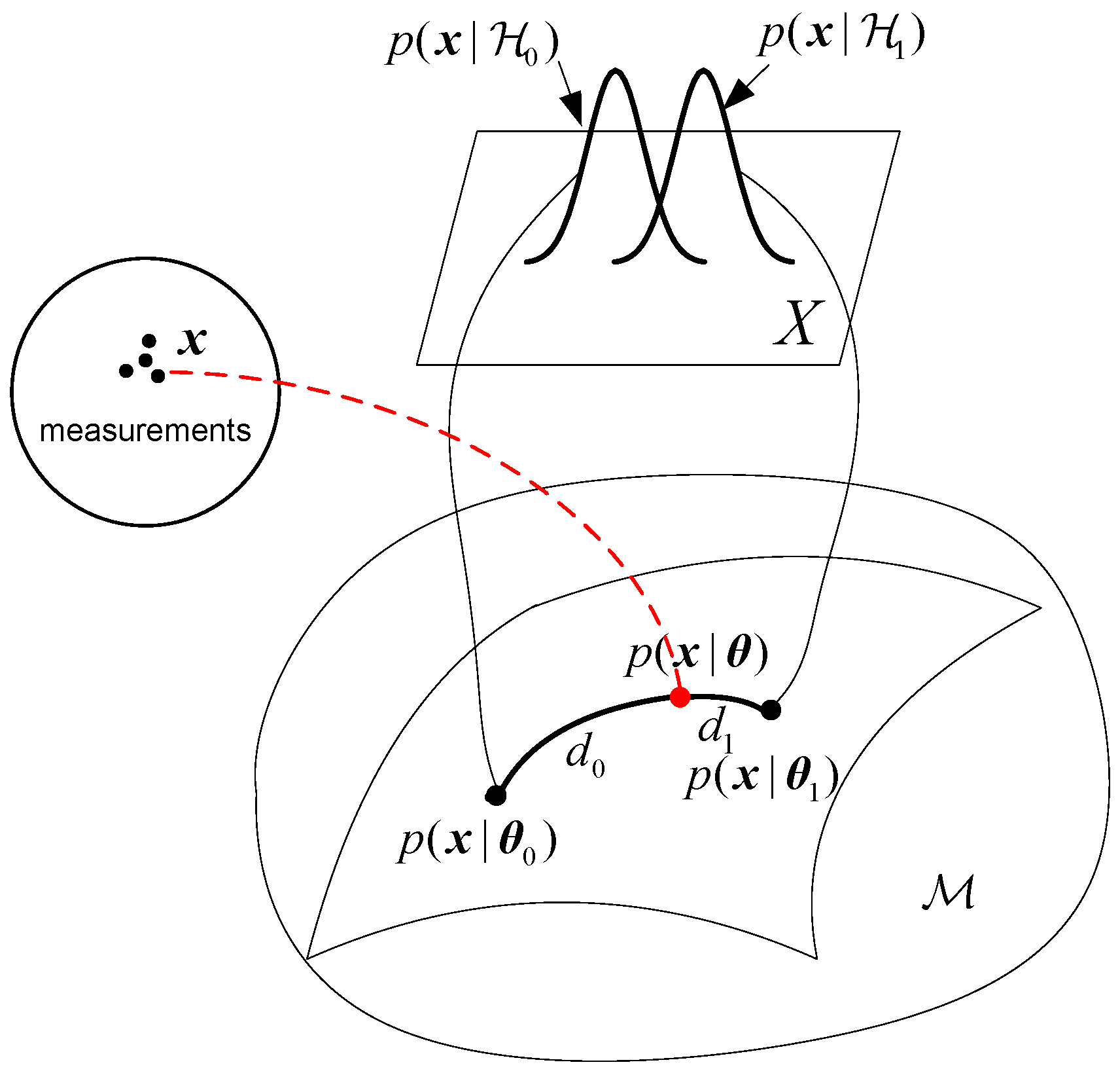
2. Geometric Interpretation of the Classical Likelihood Ratio Test
2.1. Equivalence between Likelihood Ratio Test and Kullback–Leibler Divergence
2.2. Geometric Interpretation of the Classical Likelihood Ratio Test
3. Geometry of Deterministic Signal Detection
3.1. Signal Model and Likelihood Ratio Test
3.2. Geometry of Deterministic Signal Detection
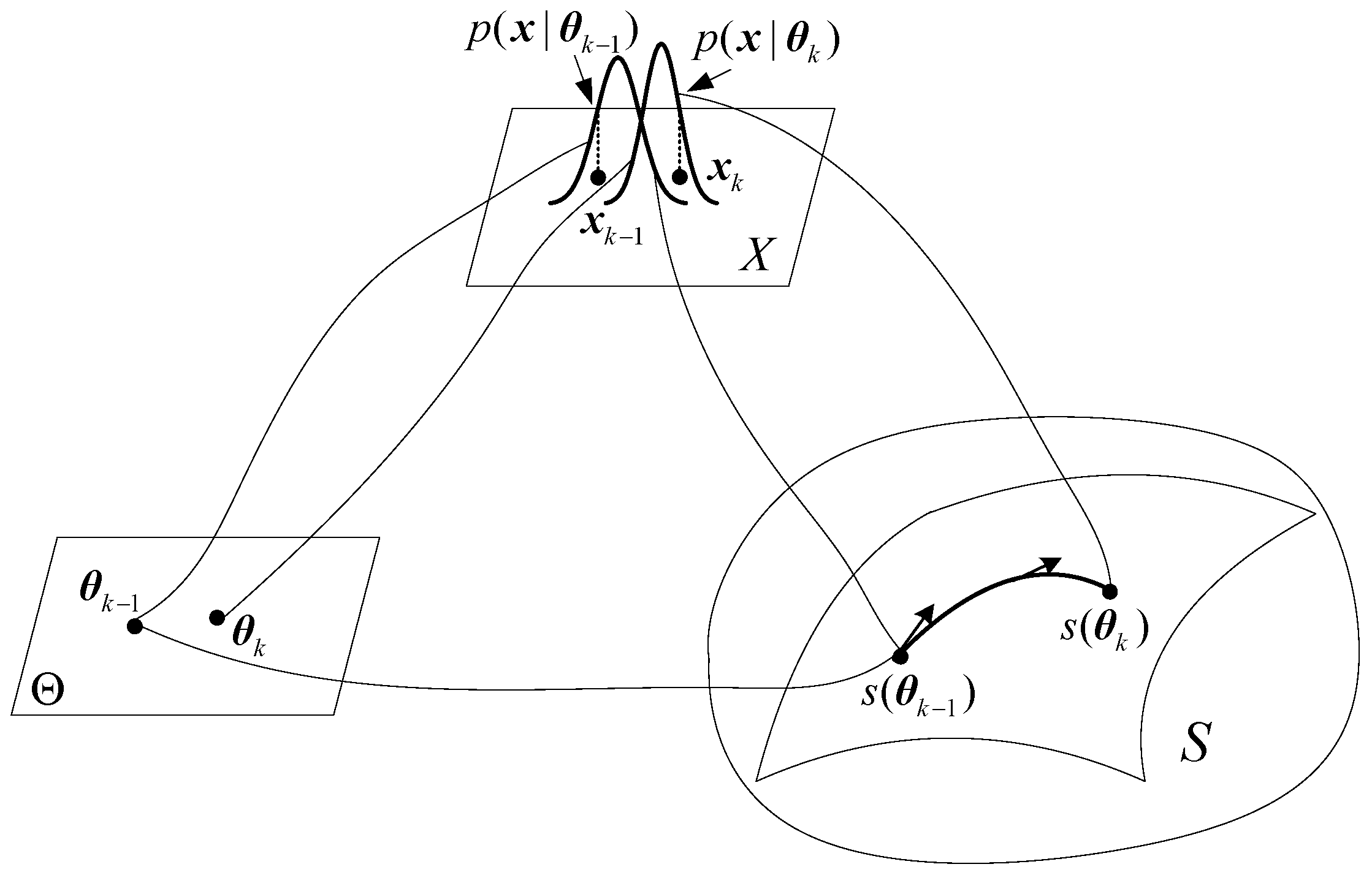
4. Geometry of Random Signal Detection
4.1. Signal Model and Likelihood Ratio Test
4.2. Geometry of Random Signal Detection
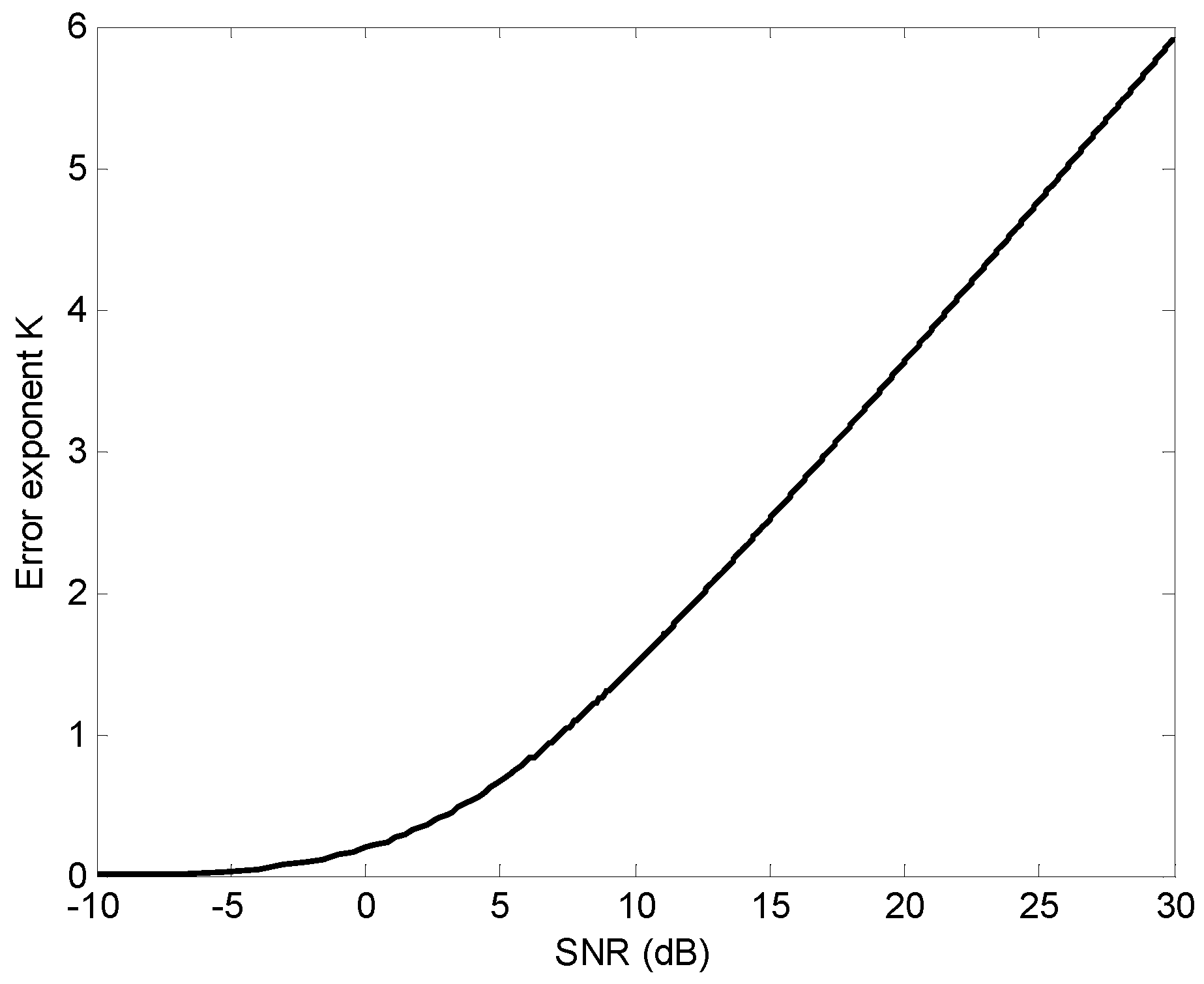
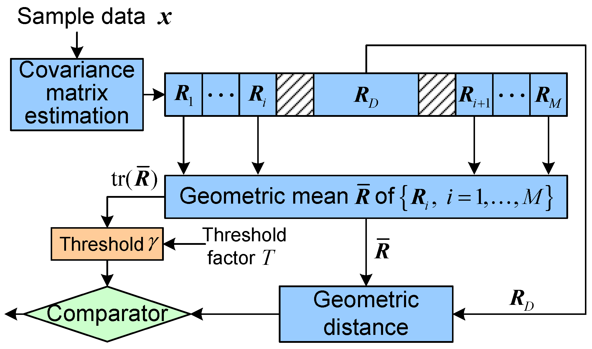
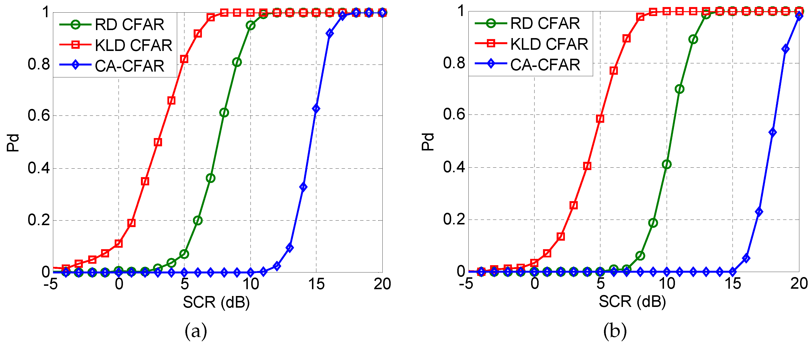
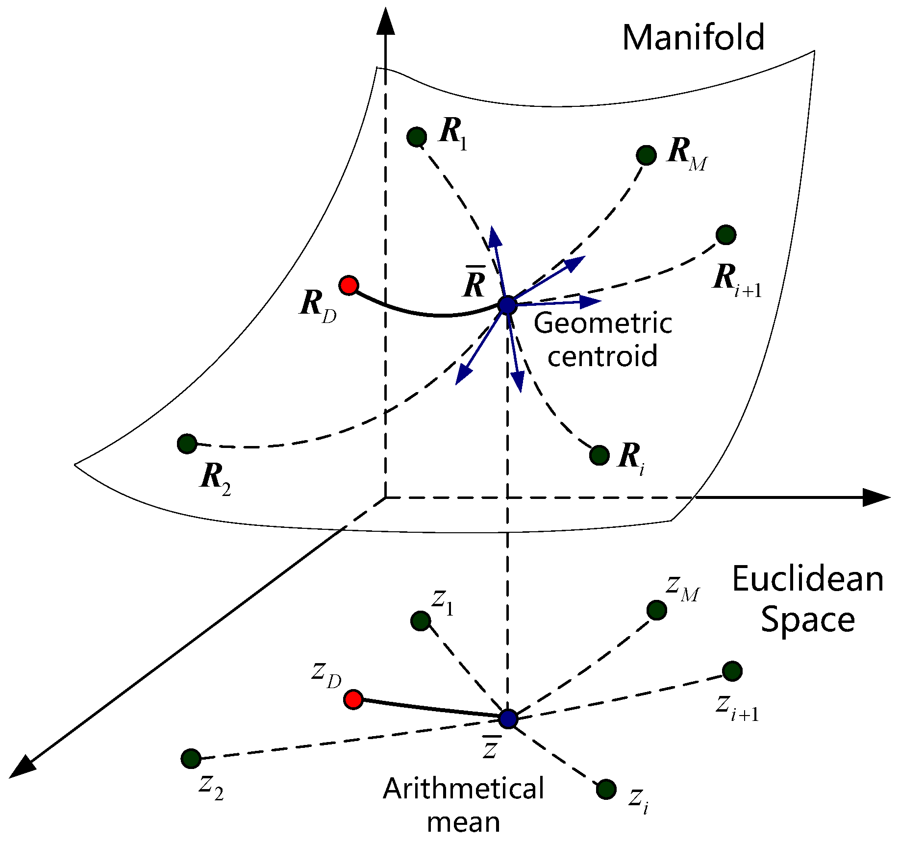
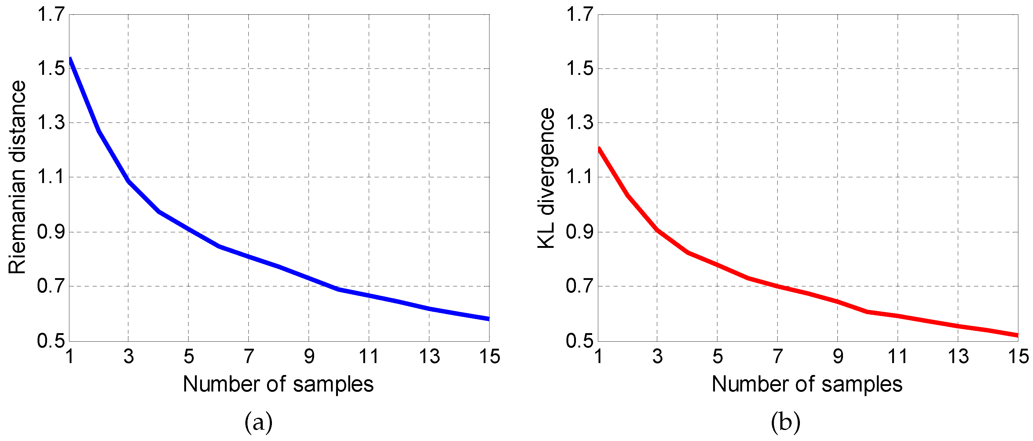
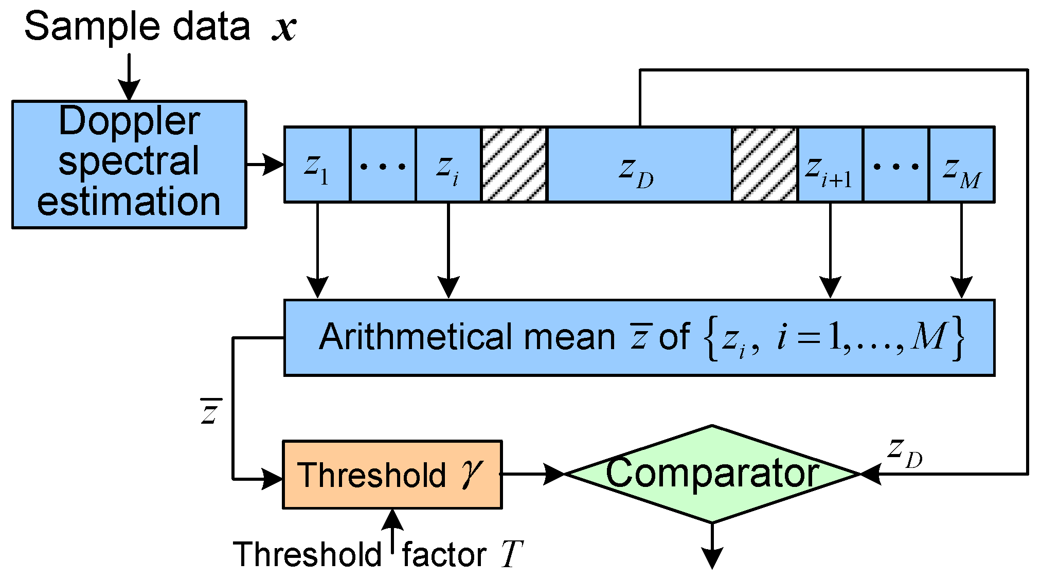
5. Application to Radar Target Detection
6. Conclusions
Acknowledgments
Author Contributions
Conflicts of Interest
References
- Kay, S.M. Fundamentals of Statistical Signal Processing: Detection Theory, 1st ed.; Prentice Hall PTR: Upper Saddle River, NJ, USA, 1993; Volume 2. [Google Scholar]
- Amari, S. Information geometry on hierarchy of probability distributions. IEEE Trans. Inf. Theory 2001, 47, 1701–1711. [Google Scholar] [CrossRef]
- Amari, S. Information geometry of statistical inference—An overview. In Proceedings of the IEEE Information Theory Workshop, Bangalore, India, 20–25 October 2002.
- Rao, C.R. Information and accuracy attainable in the estimation of statistical parameters. Bull. Calcutta Math. Soc. 1945, 37, 81–91. [Google Scholar]
- Amari, S.; Nagaoka, H. Methods of Information Geometry; Kobayashi, S., Takesaki, M., Eds.; Translations of Mathematical Monographs vol. 191; American Mathematical Society: Providence, RI, USA, 2000. [Google Scholar]
- Chentsov, N.N. Statistical Decision Rules and Optimal Inference; Leifman, L.J., Ed.; Translations of Mathematical Monographs vol. 53; American Mathematical Society: Providence, RI, USA, 1982. [Google Scholar]
- Efron, B. Defining the curvature of a statistical problem (with applications to second order efficiency). Ann. Stat. 1975, 3, 1189–1242. [Google Scholar] [CrossRef]
- Efron, B. The geometry of exponential families. Ann. Stat. 1978, 6, 362–376. [Google Scholar] [CrossRef]
- Amari, S. Differential geometry of curved exponential families-curvatures and information loss. Ann. Stat. 1982, 10, 357–385. [Google Scholar] [CrossRef]
- Kass, R.E.; Vos, P.W. Geometrical Foundations of Asymptotic Inference; Wiley: New York, NY, USA, 1997. [Google Scholar]
- Amari, S.; Kawanabe, M. Information geometry of estimating functions in semi parametric statistical models. Bernoulli 1997, 3, 29–54. [Google Scholar] [CrossRef]
- Amari, S.; Kurata, K.; Nagaoka, H. Information geometry of Boltzmann machines. IEEE Trans. Neural Netw. 1992, 3, 260–271. [Google Scholar] [CrossRef] [PubMed]
- Amari, S. Natural gradient works efficiently in learning. Neural Comput. 1998, 10, 251–276. [Google Scholar] [CrossRef]
- Amari, S. Information geometry of the EM and em algorithms for neural networks. Neural Netw. 1995, 8, 1379–1408. [Google Scholar] [CrossRef]
- Amari, S. Fisher information under restriction of Shannon information. Ann. Inst. Stat. Math. 1989, 41, 623–648. [Google Scholar] [CrossRef]
- Campbell, L.L. The relation between information theory and the differential geometry approach to statistics. Inf. Sci. 1985, 35, 199–210. [Google Scholar] [CrossRef]
- Amari, S. Differential geometry of a parametric family of invertible linear systems—Riemannian metric, dual affine connections and divergence. Math. Syst. Theory 1987, 20, 53–82. [Google Scholar] [CrossRef]
- Ohara, A.; Suda, N.; Amari, S. Dualistic differential geometry of positive definite matrices and its applications to related problems. Linear Algebra Appl. 1996, 247, 31–53. [Google Scholar] [CrossRef]
- Ohara, A. Information geometric analysis of an interior point method for semidefinite programming. In Proceedings of the Geometry in Present Day Science, Aarhus, Denmark, 16–18 January 1998; Barndorff-Nielsen, O.E., Vedel Jensen, E.B., Eds.; World Scientific: Singapore, Singapore, 1999; pp. 49–74. [Google Scholar]
- Amari, S.; Shimokawa, H. Recent Developments of Mean Field Approximation; Opper, M., Saad, D., Eds.; MIT Press: Cambridge, MA, USA, 2000. [Google Scholar]
- Richardson, T. The geometry of turbo-decoding dynamics. IEEE Trans. Inf. Theory 2000, 46, 9–23. [Google Scholar] [CrossRef]
- Li, Q.; Georghiades, C.N. On a geometric view of multiuser detection for synchronous DS/CDMA channels. IEEE Trans. Inf. Theory 2000, 46, 2723–2731. [Google Scholar]
- Smith, S.T. Covariance, subspace, and intrinsic Cramér–Rao bounds. IEEE Trans. Signal Process. 2005, 53, 1610–1630. [Google Scholar] [CrossRef]
- Srivastava, A. A Bayesian approach to geometric subspace estimation. IEEE Trans. Signal Process. 2000, 48, 1390–1400. [Google Scholar] [CrossRef]
- Srivastava, A.; Klassen, E. Bayesian and geometric subspace tracking. Adv. Appl. Probab. 2004, 36, 43–56. [Google Scholar] [CrossRef]
- Westover, M.B. Asymptotic geometry of multiple hypothesis testing. IEEE Trans. Inf. Theory 2008, 54, 3327–3329. [Google Scholar] [CrossRef]
- Varshney, K.R. Bayes risk error is a Bregman divergence. IEEE Trans. Signal Process. 2011, 59, 4470–4472. [Google Scholar] [CrossRef]
- Barbaresco, F. Innovative tools for radar signal processing based on Cartan’s geometry of SPD matrices & information geometry. In Proceedings of the 2008 IEEE Radar Conference, Rome, Italy, 26–30 May 2008.
- Barbaresco, F. New foundation of radar Doppler signal processing based on advanced differential geometry of symmetric spaces: Doppler matrix CFAR and radar application. In Proceedings of the International Radar Conference, Bordeaux, France, 12–16 October 2009.
- Barbaresco, F. Robust statistical radar processing in Fréchet metric space: OS-HDR-CFAR and OS-STAP processing in Siegel homogeneous bounded domains. In Proceedings of the International Radar Symposium, Leipzig, Germany, 7–9 September 2011.
- Etemadi, N. An elementary proof of the strong law of large numbers. Probab. Theory Relat. Fields 1981, 55, 119–122. [Google Scholar] [CrossRef]
- Kullback, S. Information Theory and Statistics; Dover Publications: New York, NY, USA, 1968. [Google Scholar]
- Cover, T.M.; Thomas, J.A. Elements of Information Theory; Wiley: New York, NY, USA, 1991. [Google Scholar]
- Pinsker, M.S. Information and Information Stability of Random Variables and Processes; Holden-Day: San Francisco, CA, USA, 1964. [Google Scholar]
- Lehmann, F.L. Testing Statistical Hypotheses; Wiley: New York, NY, USA, 1959. [Google Scholar]
- Sung, Y.; Tong, L.; Poor, H.V. Neyman–Pearson detection of Gauss-Markov signals in noise: Closed-form error exponent and properties. IEEE Trans. Inf. Theory 2006, 52, 1354–1365. [Google Scholar] [CrossRef]
- Chamberland, J.; Veeravalli, V.V. Decentralized detection in sensor networks. IEEE Trans. Signal Process. 2003, 51, 407–416. [Google Scholar] [CrossRef]
- Sullivant, S. Statistical Models Are Algebraic Varieties. Available online: https://www.researchgate.net/profile/Seth_Sullivant/publication/254069909_Statistical_Models_are_Algebraic_Varieties/links/552bdb0d0cf2e089a3aa889a.pdf?origin=publication_detail (accessed on 13 April 2015).
- Moakher, M. A differential geometric approach to the geometric mean of symmetric positive-definite matrices. SIAM J. Matrix Anal. Appl. 2005, 26, 735–747. [Google Scholar] [CrossRef]
- Balaji, B.; Barbaresco, F.; Decurninge, A. Information geometry and estimation of Toeplitz covariance matrices. In Proceedings of the 2014 International Radar Conference, Lille, France, 13–17 October 2014.
- Conte, E.; Lops, M.; Ricci, G. Asymptotically optimum radar detection in compound-Gaussian clutter. IEEE Trans. Aerosp. Electron. Syst. 1995, 31, 617–625. [Google Scholar] [CrossRef]
- Roy, L.P.; Kumar, R.V.R. A GLRT detector in partially correlated texture based compound-Gaussian clutter. In Proceedings of the 2010 National Conference on Communications (NCC), Chennai, India, 29–31 January 2010.
- Vela, G.M.; Portas, J.A.B.; Corredera, J.R.C. Probability of false alarm of CA-CFAR detector in Weibull clutter. Electron. Lett. 1998, 34, 806–807. [Google Scholar] [CrossRef]


© 2016 by the authors; licensee MDPI, Basel, Switzerland. This article is an open access article distributed under the terms and conditions of the Creative Commons Attribution (CC-BY) license (http://creativecommons.org/licenses/by/4.0/).
Share and Cite
Cheng, Y.; Hua, X.; Wang, H.; Qin, Y.; Li, X. The Geometry of Signal Detection with Applications to Radar Signal Processing. Entropy 2016, 18, 381. https://doi.org/10.3390/e18110381
Cheng Y, Hua X, Wang H, Qin Y, Li X. The Geometry of Signal Detection with Applications to Radar Signal Processing. Entropy. 2016; 18(11):381. https://doi.org/10.3390/e18110381
Chicago/Turabian StyleCheng, Yongqiang, Xiaoqiang Hua, Hongqiang Wang, Yuliang Qin, and Xiang Li. 2016. "The Geometry of Signal Detection with Applications to Radar Signal Processing" Entropy 18, no. 11: 381. https://doi.org/10.3390/e18110381
APA StyleCheng, Y., Hua, X., Wang, H., Qin, Y., & Li, X. (2016). The Geometry of Signal Detection with Applications to Radar Signal Processing. Entropy, 18(11), 381. https://doi.org/10.3390/e18110381