Entropy Cross-Efficiency Model for Decision Making Units with Interval Data

Abstract

The cross-efficiency method, as a Data Envelopment Analysis (DEA) extension, calculates the cross efficiency of each decision making unit (DMU) using the weights of all decision making units (DMUs). The major advantage of the cross-efficiency method is that it can provide a complete ranking for all DMUs. In addition, the cross-efficiency method could eliminate unrealistic weight results. However, the existing cross-efficiency methods only evaluate the relative efficiencies of a set of DMUs with exact values of inputs and outputs. If the input or output data of DMUs are imprecise, such as the interval data, the existing methods fail to assess the efficiencies of these DMUs. To address this issue, we propose the introduction of Shannon entropy into the cross-efficiency method. In the proposed model, intervals of all cross-efficiency values are firstly obtained by the interval cross-efficiency method. Then, a distance entropy model is proposed to obtain the weights of interval efficiency. Finally, all alternatives are ranked by their relative Euclidean distance from the positive solution.

1. Introduction

When decision making units (DMUs) have multiple inputs and outputs, data envelopment analysis (DEA) is a well-known non-parametric programming technique for assessing the efficiency of these DMUs. The maximum of the ratio of a DMU’s weighted sum of outputs to its weighted sum of inputs is defined as the efficiency score of this DMU. If the efficiency score of a DMU is equal to 1, it is considered as efficient. Otherwise, it is inefficient. Usually, inefficient DMUs are considered as performing worse than efficient ones. Since DEA was proposed by Charnes et al. [1], it has been widely applied to various cases of performance evaluation [2,3,4,5,6,7]. DEA models (both CCR (Charnes, Cooper and Rhodes) and BCC (Banker, Charnes, and Cooper) models) classify units into two groups: efficient and inefficient in the Pareto sense (see Sinuay-Shten et al. [8]). In addition, DEA is not able to rank the efficient DMUs that all have an efficiency score of 1. In order to solve this problem, the cross-efficiency method was developed by Sexton et al. [9]. The cross-efficiency method, as a DEA extension, could obtain the efficiency of each DMU by linking the weights of all DMUs. Its primary advantage is that all DMUs can be completely ranked [10]. In addition, the cross-efficiency method could eliminate unrealistic weight results [11].

With these advantages, the cross-efficiency evaluation has been extensively applied in various performance evaluation problems [12,13,14,15]. In spite of its wide applications, cross-efficiency evaluation still has some defects, such as non-uniqueness of the DEA optimal weights [9]. Usually, the optimal weights obtained by traditional DEA models are non-unique. If a set of weights are selected arbitrarily, then cross-efficiency scores will be arbitrarily generated [16]. To solve the problem of weight non-uniqueness, Sexton et al. [9] improved the cross-efficiency evaluation method by incorporating a secondary goal model. Following the idea of Sexton et al. [9], a number of scholars have proposed secondary goal models. For example, Liang et al. [17] proposed three secondary goal models, and each secondary goal corresponds to a practical case scenario. Based on the models of Liang et al. [17], Wang and Chin [18] proposed the improved models by replacing the target efficiency. Jahanshahloo et al. [19] improved traditional cross-efficiency evaluation by considering symmetric weights. Wu et al. [20] and Contreras [21] proposed improving the ranking position of the evaluated DMU when choosing weights. In the study of Lim [22], the secondary goal was proposed to minimize (or maximize) the cross efficiencies of evaluated DMUs. Maddahi et al. [23] proposed a proportional weight assignment secondary goal, making weights be assigned proportionally to input or output evaluated DMUs. In these secondary models, most models are benevolent or aggressive. In the benevolent (aggressive) model, the selected weights for evaluated DMUs are to make the cross-efficiencies of other DMUs as large (small) as possible. Different from the above ideas, scholars also have proposed new cross-efficiency models from different perspectives. For example, Cook and Zhu [24] proposed a units-invariant multiplicative DEA model, directly generating the unique cross-efficiency scores. Based on the Pareto optimality, Wu et al. [25] proposed the Pareto improvement cross-efficiency evaluation, which could obtain Pareto-optimal cross efficiencies for all DMUs.

Besides secondary goals in the cross-efficiency evaluation, scholars also have examined aggregating cross-efficiencies for obtaining cross-efficiency matrix. For example, Wu et al. [26] introduced Shapley cooperative game theory into cross-efficiency evaluation, considering each DMU as a player, and proposed a Shapley DEA model to obtain all the weights of cross-efficiencies. Wang et al. [27] considered that all cross-efficiencies of DMUs should have different preference weights. From the preference deviation degree, they proposed three different models for aggregating cross-efficiencies. Angiz et al. [28] argued that the DMU may be more concerned about whether the assigned weights improve their ranking when weights are selected for their cross-efficiencies. Based on this idea, they proposed a ranking preference model. Yang et al. [29] regarded the cross-efficiency as the independent evidence, and thus the evidence reasoning method was used to aggregate cross-efficiencies.

The traditional DEA or cross-efficiency models assume that the data of DMUs are known exactly. However, because of the existence of uncertainty, the data may be given in a fuzzy form. Therefore, a number of studies examined how to evaluate the efficiencies of DMUs with fuzzy data. For example, Cooper et al. [30] proposed an imprecise DEA (IDEA) model, which can be transformed into a linear programming model based on a series of variable alternations and scale transformations. However, Lee et al. [31] argued that IDEA model was complicated, and may lead to a rapid increase in computation burden. To solve this problem, Despotis and Smirlis [32] proposed two improved models. Through these two improved models, the lower and upper efficiency of each DMU could be obtained. Wang et al. [33] pointed out that Despotis and Smirlis’s model [32] used two different production frontiers to measure the efficiencies of DMUs, and this may lead to the efficiencies of DMUs’ lack of comparability. To deal with such an issue, Wang et al. [33] proposed the new DEA models based on a common frontier to obtain the interval efficiency of each DMU and a minimax regret-based approach was then used for ranking the interval efficiencies of all DMUs. To determine the range of interval efficiency of each DMU, Azizi and Jahed [34] introduced a virtual ideal DMU into the DEA model. The efficiency of ideal DMU is definitely the largest among all the DMUs, so the worst and the best relative efficiencies of each DMU can be obtained. Then, the worst and the best relative efficiencies constitute an interval for the overall performance evaluation of each DMU. Wang and Chin [35] proposed the fuzzy DEA models based on two pairs of expected value models to measure the optimistic and the pessimistic efficiencies of DMUs. They integrated two extreme efficiencies through a geometric average for obtaining the overall performances of the DMUs. Dotoli et al. [36] proposed a novel approach by integrating the DEA cross-efficiency technique with the fuzzy logic framework. This approach not only maintains the cross-efficiency DEA discriminative power but also deals with uncertainty.

Although the existing cross-efficiency methods have well examined how to be aggressive or benevolent to DMUs when evaluating the efficiencies, the maximum discrimination of DMUs has been largely ignored. In addition, there is a paucity of research on aggregating interval cross-efficiency matrices. To fill these gaps, the present study proposes a new cross-efficiency method based on the entropy theory. In this new approach, the model of Wang et al. [33] is first extended into cross-efficiency evaluation to obtain the intervals of all cross-efficiency values. Then, the DEA entropy model is used to calculate the weights of all interval cross-efficiencies. Finally, all DMUs are evaluated and ranked according to the distance to ideal positive cross-efficiency. This approach is illustrated and verified by a demonstrative case using data from China’s primary schools. We conclude that the proposed approach is effective to evaluate DMUs with interval data and can provide complete and fair results for all DMUs.

The rest of the paper is organized as follows. Section 2 introduces the interval DEA models and Section 3 presents the cross-efficiency evaluation method with interval data. The cross-efficiency model based on Shannon entropy is discussed in Section 4, followed by a numerical demonstration using data from Chinese primary schools in Section 5. Conclusions are presented in Section 6.

2. Interval DEA Models

There are n DMUs to be evaluated, and each DMU has s different outputs and m different inputs. Input i and output r for $DM{U}_j$ are denoted as $x_{ij}$ and $y_{rj}$, respectively. The input and output data may be imprecise because of uncertainty and thus only their bounded intervals $[x_{ij}^l,x_{ij}^u]$ and $[y_{rj}^l,y_{rj}^u]$, with $x_{ij}^l>0$ and $y_{rj}^l>0$, are provided. For measuring the efficiencies of the DMUs with interval data, Despotis and Smirlis [32] proposed a linear problem model to generate the lower and upper bounds of the efficiency for each DMU, as shown in Model (1):

$$\begin{array}{l}\max E_{dd}=\frac{{\displaystyle \sum _{r=1}^s{\mu }_{rd}}[y_{rd}^l,y_{rd}^u]}{{\displaystyle \sum _{j=1}^m{\omega }_{id}}[x_{id}^l,x_{id}^u]}\\ s.t.\frac{{\displaystyle \sum _{r=1}^s{\mu }_{rd}}[y_{rd}^l,y_{rd}^u]}{{\displaystyle \sum _{j=1}^m{\omega }_{id}}[x_{id}^l,x_{id}^u]}\le 1,j=1,2,\cdots ,n\\ {\omega }_{id},{\mu }_{rd}\ge \epsilon \forall id,rd\end{array}.$$

(1)

However, Wang et al. [33] pointed out that Despotis and Smirlis [32] used two different production frontiers to obtain interval efficiency, and thus all DMUs cannot be compared on the basis of a common evaluation criterion. In order to calculate the lower and upper bound of the efficiency of $DM{U}_d$, Wang et al. [33] proposed two linear formulations to generate the bounded interval $[E_{dd}^l,E_{dd}^u]$, as follows:

$$\begin{array}{l}\max E_{dd}^l={\displaystyle \sum _{r=1}^s{\mu }_{rd}}{y}_{rd}^l\\ s.t.{\displaystyle \sum _{i=1}^m{\omega }_{id}}{x}_{ij}^l-{\displaystyle \sum _{r=1}^s{\mu }_{rd}}{y}_{rj}^u\ge 0,j=1,2,\cdots ,n\\ {\displaystyle \sum _{j=1}^m{\omega }_{id}}{x}_{id}^u=1\\ {\omega }_{id},{\mu }_{rd}\ge \epsilon ,\forall id,rd\end{array},$$

(2)

and

$$\begin{array}{l}\max E_{dd}^u={\displaystyle \sum _{r=1}^s{\mu }_{rd}}{y}_{rd}^u\\ s.t.{\displaystyle \sum _{i=1}^m{\omega }_{id}}{x}_{ij}^l-{\displaystyle \sum _{r=1}^s{\mu }_{rd}}{y}_{rj}^u\ge 0,j=1,2,\cdots ,n\\ {\displaystyle \sum _{i=1}^m{\omega }_{id}}{x}_{id}^l=1\\ {\omega }_{id},{\mu }_{rd}\ge \epsilon ,\forall id,rd\end{array}.$$

(3)

In Models (2) and (3), $DM{U}_d$ is to be evaluated. ${\omega }_{id}$ and ${\mu }_{rd}$ are the weights of the input i and output r, respectively. $E_{dd}^l$ (or $E_{dd}^u$) is the lower (or upper) efficiency for $DM{U}_d$. $\epsilon$ is the non-Archimedean infinitesimal. From Models (2) and (3), it is clear that $E_{dd}^l\le E_{dd}^u$.

3. Cross-Efficiency Evaluation Method with Interval Data

Models (2) and (3) are the self-assessment models. The self-evaluated DEA model enables each DMU to choose the most favorable weights for evaluating its efficiency. This may lead to more than one DMU is assessed as efficient, and such DEA-efficient DMUs cannot be further distinguished (Wang and Chin, [37]). To solve this problem, Sexton et al. [9] proposed a cross-efficiency DEA method by introducing the concept of peer evaluation. However, the method of Sexton et al. [9] has a problem of multiple optimum weight solutions. A weight scheme obtained by Sexton et al. [9] may be favorable to one DMU, but not to another. To address this ambiguity of weight selection, Doyle and Green [10] proposed the aggressive and benevolent formulations by introducing a secondary goal into the cross-efficiency method. In the case of aggressive (or benevolent) formulation, the secondary goal could choose the weights to make the efficiency of the target DMU the best that it can be, and all other DMUs worst (or best). However, Oukil and Amin [38] pointed out that the aggressive and benevolent models of Doyle and Green [10] used a common set of weights for all DMUs, which would not guarantee maximum discrimination among DMUs. To improve discrimination, Oukil and Amin [38] proposed using different weights for cross-efficiency scores. The purpose of our present study is to effectively discriminate all DMUs with interval data. Therefore, our study adopts the viewpoint of Oukil and Amin [38]. In our study, the model [33] is extended to obtain the lower and upper cross-efficiencies for each DMU. Model (4) can calculate the low cross-efficiency values for interval data:

$$\begin{array}{l}\max {\displaystyle \sum _{r=1}^s{\mu }_{rd}{y}_{rj}^l}\\ s.t.{\displaystyle \sum _{i=1}^m{\omega }_{id}}{x}_{ij}^l-{\displaystyle \sum _{r=1}^s{\mu }_{rd}}{y}_{rj}^u\ge 0,j=1,2,\cdots ,n\\ {\displaystyle \sum _{i=1}^m{\omega }_{id}{x}_{ij}^u}=1\\ E_{dd}^l\times {\displaystyle \sum _{j=1}^m{\omega }_{id}}{x}_{id}^u-{\displaystyle \sum _{r=1}^s{\mu }_{rd}}{y}_{rd}^l=0\\ {\omega }_{id},{\mu }_{rd}\ge \epsilon ,\forall id,rd\end{array}.$$

(4)

Similarly, the upper cross-efficiency values of interval data can be computed with Model (5):

$$\begin{array}{l}\max {\displaystyle \sum _{r=1}^s{\mu }_{rd}{y}_{rj}^u}\\ s.t.{\displaystyle \sum _{i=1}^m{\omega }_{id}}{x}_{ij}^l-{\displaystyle \sum _{r=1}^s{\mu }_{rd}}{y}_{rj}^u\ge 0,j=1,2,\cdots ,n\\ {\displaystyle \sum _{i=1}^m{\omega }_{id}{x}_{ij}^l}=1\\ E_{dd}^u\times {\displaystyle \sum _{j=1}^m{\omega }_{id}}{x}_{id}^l-{\displaystyle \sum _{r=1}^s{\mu }_{rd}}{y}_{rd}^u=0\\ {\omega }_{id},{\mu }_{rd}\ge \epsilon ,\forall id,rd\end{array}.$$

(5)

After all cross-efficiency values are computed, an interval efficiency matrix can be obtained as shown in

Table 1. A generalized interval cross-efficiency matrix.

Rating $\mathit{D}\mathit{M}{\mathit{U}}_{\mathit{d}}$	Rated $\mathit{D}\mathit{M}{\mathit{U}}_{\mathit{j}}$
	1	2	3	…	n
1	[$E_{11}^l$,$E_{11}^u$]	[$E_{12}^l$,$E_{12}^u$]	[$E_{13}^l$,$E_{13}^u$]	…	[$E_{1n}^l$,$E_{1n}^u$]
2	[$E_{21}^l$,$E_{21}^u$]	[$E_{22}^l$,$E_{22}^u$]	[$E_{23}^l$,$E_{23}^u$]	…	[$E_{2n}^l$,$E_{2n}^u$]
3	[$E_{31}^l$,$E_{31}^u$]	[$E_{32}^l$,$E_{32}^u$]	[$E_{33}^l$,$E_{33}^u$]	…	[$E_{3n}^l$,$E_{3n}^u$]
…	…	…	…	…	…
n	[$E_{n1}^l$,$E_{n1}^u$]	[$E_{n2}^l$,$E_{n2}^u$]	[$E_{n3}^l$,$E_{n3}^u$]	…	[$E_{nn}^l$,$E_{nn}^u$]

. In each column, [$E_{dj}^l$,$E_{dj}^u$] represents the lower and upper bounds of the cross-efficiency scores of $DM{U}_j$ by using the weights of $DM{U}_d$.

Models (4) and (5) are built upon the classical cross-efficiency DEA framework, and we consider only the CRS (constant returns to scale) condition in the present study. Models (4) and (5) are inappropriate to be extended to the case of VRS (variable returns to scale). The reason is that integrating the concept of the VRS into the cross-efficiency DEA framework may yield negative cross-efficiency scores (Cook and Zhu [39] and Lim and Zhu [40]).

The DEA method mainly has two orientation modes—inputs and outputs. Under the form of the multiplier DEA model, the input orientation mode is expressed as maximizing the ratio of the DMU’s sum of weighted outputs to its sum of weighted inputs. Output orientation mode is formulated as maximizing the ratio of the DMU’s sum of weighted inputs to its sum of weighted outputs (Cooper et al. [41] and Cook and Bala [42]). Therefore, per these definitions, Models (4) and (5) are input orientation modes.

4. The Cross-Efficiency Model Based on Shannon Entropy

Shannon entropy is a useful and effective mathematical concept for measuring uncertainty [43]. Incorporating Shannon entropy into DEA has attracted the interests of a number of scholars [44,45,46]. In this section, Shannon entropy is utilized to calculate the weights of interval cross-efficiency. The weights are obtained by making the distance between the self-evaluation entropy score and peer evaluation entropy score as small as possible. The cross-efficiency entropy model is proposed as in the following steps:

• Step 1: Determining the entropy value of interval cross-efficiency.

As defined in Table 1, $E=(E_{ij}^l,E_{ij}^u)|(E_{ij}^l\in R_{+}^{n\times n},E_{ij}^u\in R_{+}^{n\times n})$ is the interval cross-efficiency matrix, and the elements $E_{dj}^l$ and $E_{dj}^u$ represent the interval efficiency that $DM{U}_d$ accords to $DM{U}_j$. After normalizing the matrix E, the entropy value of interval cross-efficiency can be defined as follows:

Definition 1.

For $DM{U}_j$, the lower (or upper) entropy value of lower (or upper) cross-efficiency score is defined as:

$$h_{ij}^l=-D_{ij}^l\ln D_{ij}^l,$$

(6)

$$h_{ij}^u=-D_{ij}^u\ln D_{ij}^u,$$

(7)

where $D_{ij}^l=\frac{E_{ij}^l}{{\displaystyle \sum _{i=1}^n{E}_{ij}^l}}$ and $D_{ij}^u=\frac{E_{ij}^u}{{\displaystyle \sum _{i=1}^n{E}_{ij}^u}}$.

Theorem 1.

Entropy values can be added.

For each $DMU$ (e.g., $DM{U}_j$), it has n lower cross-efficiency scores ($E_{ij}^l$, $i=1,2,\cdots ,n$) and n upper cross-efficiency scores ($E_{ij}^u$, $i=1,2,\cdots ,n$). After Step 1, the lower (or upper) entropy of $DM{U}_j$ is equal to the sum of its n entropy cross-efficiency scores. That is,

$$H_j^l={\displaystyle \sum _{i=1}^n{h}_{ij}^l}=-{\displaystyle \sum _{i=1}^n{D}_{ij}^l\ln D_{ij}^l}\mathrm{or}{H}_j^u={\displaystyle \sum _{i=1}^n{h}_{ij}^u}=-{\displaystyle \sum _{i=1}^n{D}_{ij}^u\ln D_{ij}^u}.$$

• Step 2: Calculating the weights based on the proposed cross-efficiency entropy model.

Definition 2.

For $DM{U}_j$, the distance entropy function between cross-efficiency score and its self-evaluation efficiency score is defined as:

$$b_{ij}^l=h_{jj}^{l*}-h_{ij}^l,i=1,2,\cdots ,n,$$

(8)

$$b_{ij}^u=h_{jj}^{u*}-h_{ij}^u,i=1,2,\cdots ,n,$$

(9)

where $h_{ij}^l$ (or $h_{ij}^u$) and $h_{jj}^{l*}$ (or $h_{jj}^{u*}$) are the entropy values of cross-efficiency score $E_{ij}^l$ (or $E_{ij}^u$) and efficiency score $E_{jj}^l$ (or $E_{jj}^u$) of Models (2) or (3), respectively. Entropy is a measurement of uncertainty, and we assume that the reasonable weights should make distance entropy of all cross-efficiencies be the smallest and thus uncertainty of interval cross-efficiency would be the smallest. Therefore, cross-efficiency entropy model are as follows:

$$\begin{array}{cc}\hfill \min Z& ={\displaystyle \sum _{j=1}^n{\displaystyle \sum _{i=1}^n{(b_{ij}^l)}^2{\lambda }_i^2}}+{\displaystyle \sum _{j=1}^n{\displaystyle \sum _{i=1}^n{(b_{ij}^u)}^2{\lambda }_i^2}}\hfill \\ & ={\displaystyle \sum _{j=1}^n{\displaystyle \sum _{i=1}^n{(h_{jj}^{l*}-h_{ij}^l)}^2{\lambda }_i^2}}+{\displaystyle \sum _{j=1}^n{\displaystyle \sum _{i=1}^n{(h_{jj}^{u*}-h_{ij}^u)}^2{\lambda }_i^2}}\\ & ={\displaystyle \sum _{j=1}^n{\displaystyle \sum _{i=1}^n[{(h_{jj}^{l*}-h_{ij}^l)}^2+{(h_{jj}^{u*}-h_{ij}^u)}^2]{\lambda }_i^2}}\\ \hfill s.t.& {\displaystyle \sum _{i=1}^n{\lambda }_i}=1\hfill \\ & {\lambda }_i>0(j=1,\cdots ,n)\hfill \end{array}.$$

(10)

Model (10) essentially is a multi-attribute decision making method. According to characteristics of multi-attribute decision making model (Wang and Parkan [47], Wang and Luo [48], and Tzeng and Huang [49]), the sum of weights is equal to 1. Therefore, the weights ${\lambda }_i$ in Model (10) also need to satisfy this constraint. Then, according to Lagrangian sufficiency theorem, the weight ${\lambda }_i$ can be determined as follows:

$${\lambda }_i=\frac{{\left\{{\displaystyle \sum _{j=1}^n[{(h_{jj}^{l*}-h_{ij}^l)}^2+{(h_{jj}^{u*}-h_{ij}^u)}^2]}\right\}}^{-1}}{{\displaystyle \sum _{i=1}^n({\displaystyle \sum _{j=1}^n[{(h_{jj}^{l*}-h_{ij}^l)}^2+{(h_{jj}^{u*}-h_{ij}^u)}^2]{)}^{-1}}}}.$$

(11)

• Step 3: Determining the weighted normalization decision matrix.

The weighted normalization value is calculated by

$$V_{ij}^l={\lambda }_i*E_{ij}^l,V_{ij}^u={\lambda }_i*E_{ij}^u,$$

(12)

where ${\lambda }_i$ is the weight of attribute $j$, for all $i=1,2,\cdots ,n\mathrm{and}j=1,2,\cdots ,n$.

• Step 4: Determining the positive ideal solutions.

After Step 3, there are two weighted normalization matrix ($V_{ij}^l$ and $V_{ij}^u$). In this step, the maximum value of each row in each matrix is found as the positive ideal solution:

$$v_i^{l*}=\underset{1\le j\le n}{\max }{v}_{ij}^l,i=1,2,\cdots ,n,v_i^{u*}=\underset{1\le j\le n}{\max }{v}_{ij}^u,i=1,2,\cdots ,n.$$

(13)

• Step 5: Calculating the Euclidean distance from the positive solutions:

$$d_j^{u*}={\displaystyle \sum _{i=1}^n{(v_{ij}^u-v_i^{u*})}^2},d_j^{l*}={\displaystyle \sum _{i=1}^n{(v_{ij}^l-v_i^{l*})}^2},d_j^{*}=d_j^{u*}+d_j^{l*}.$$

(14)

Therefore, the final distance from the positive solutions is $d_j^{*}$.

• Step 6: Determining the rank of all alternatives on the basis of their relative Euclidean distance from the positive solutions.

The smaller the $d_j$ is, the better the alternative $A_i$ will be. The best alternative is the one with the smallest relative Euclidean distance to the ideal solutions.

Theorem 2.

The constraints of Model (10) are non-empty convex set.

Proof. 

Let C be the constraints of Model (7). It is evident that C is non-empty. Now, assume both $({\lambda }_1^{\prime },\cdots ,{\lambda }_n^{\prime })$ and $({\lambda }_1^{″},\cdots ,{\lambda }_n^{″})\in C$. For any $\beta \in [0,1]$, we have $\beta {\lambda }_i^{\prime }+(1-\beta ){\lambda }_i^{″}\in C$. Therefore, C is convex.  □

Theorem 3.

The objective function $Z={\displaystyle \sum _{j=1}^n{\displaystyle \sum _{i=1}^n{(b_{ij}^l)}^2{\lambda }_i^2}}+{\displaystyle \sum _{j=1}^n{\displaystyle \sum _{i=1}^n{(b_{ij}^u)}^2{\lambda }_i^2}}$ is a convex function in the definition domain.

Proof. 

For $C\subset R_{+}^n$ and C is a non-empty convex set, the objective function $Z={\displaystyle \sum _{j=1}^n{\displaystyle \sum _{i=1}^n{(b_{ij}^l)}^2{\lambda }_i^2}}+{\displaystyle \sum _{j=1}^n{\displaystyle \sum _{i=1}^n{(b_{ij}^u)}^2{\lambda }_i^2}}$ has the continuous second partial derivatives. The Hessian matrix of the objective function is:

$$\left[\begin{array}{cccc}\frac{{\partial }_z^2}{\partial {\lambda }_1\partial {\lambda }_1}& \frac{{\partial }_z^2}{\partial {\lambda }_1\partial {\lambda }_2}& \cdots & \frac{{\partial }_z^2}{\partial {\lambda }_1\partial {\lambda }_n}\\ \frac{{\partial }_z^2}{\partial {\lambda }_2\partial {\lambda }_1}& \frac{{\partial }_z^2}{\partial {\lambda }_2\partial {\lambda }_2}& \cdots & \frac{{\partial }_z^2}{\partial {\lambda }_2\partial {\lambda }_n}\\ \cdots & \cdots & \cdots & \cdots \\ \frac{{\partial }_z^2}{\partial {\lambda }_n\partial {\lambda }_1}& \frac{{\partial }_z^2}{\partial {\lambda }_n\partial {\lambda }_2}& \cdots & \frac{{\partial }_z^2}{\partial {\lambda }_n\partial {\lambda }_n}\end{array}\right]=\left[\begin{array}{cccc}2{\displaystyle \sum _{j=1}^n[{(b_{1j}^l)}^2+{(b_{1j}^u)}^2]}& 0& \cdots & 0\\ 0& 2{\displaystyle \sum _{j=1}^n[{(b_{2j}^l)}^2+{(b_{2j}^u)}^2]}& \cdots & 0\\ \cdots & \cdots & \cdots & \cdots \\ 0& 0& \cdots & 2{\displaystyle \sum _{j=1}^n[{(b_{nj}^l)}^2+{(b_{nj}^u)}^2]}\end{array}\right].$$

(15)

Hessian matrix is always positive definite. Therefore, the objective function is a strongly convex function.  □

Theorem 4.

${\lambda }_i^{*}$ is the global optimal solution of Model (10).

Proof. 

C is a non-empty convex set, the objective function $Z={\displaystyle \sum _{j=1}^n{\displaystyle \sum _{i=1}^n{(b_{ij}^l)}^2{\lambda }_i^2}}+{\displaystyle \sum _{j=1}^n{\displaystyle \sum _{i=1}^n{(b_{ij}^u)}^2{\lambda }_i^2}}$ is a convex function, thus Model (10) is a convex programming model, and the generated ${\lambda }_i^{*}$ is the global optimal solution of Model (10).  □

5. Illustrations

5.1. The Case of Primary Schools

The illustrative application uses a dataset of all primary schools in China’s Jinhu County, Jiangsu, China. To be consistent with extant studies in the literature, we choose input variables as the number of staff, school building area (in Square meters), copies of books, fixed assets (in 10⁶ RMB), and school budget (in 10⁶ RMB). The output variable is the number of students in each school. All the data was collected from the Education Bureau of Jinhu County. The school profile is shown in

Table 2. The data of input and output of all schools.

School	Number of Staff	School Building Area (Square meters)	Copies of Books	Fixed Asset (Million RMB)	School Budget (Million RMB)	Number of Students
1	[47,53]	3964	8947	3.54	9.26	[313,360]
2	[39,40]	965	4247	2.04	3.41	[102,110]
3	[65,70]	2222	8543	2.23	12.07	[263,300]
4	[43,54]	2316	7560	2.42	5.70	[261,274]
5	[47,49]	3362	11,035	1.23	5.90	[292,312]
6	[49,59]	3273	6120	5.61	8.53	[261,289]
7	[30,36]	1534	7439	2.55	5.73	[256,270]
8	[45,57]	1130	4043	2.25	10.07	[73,81]
9	[38,45]	2278	7306	1.51	7.60	[293,311]
10	[104,124]	7321	25,218	16.91	15.73	[1129,1195]
11	[92,110]	6218	11,552	10.86	13.95	[410,455]
12	[38,40]	1878	4155	3.89	6.43	[191,202]
13	[42,46]	2649	6986	1.41	6.22	[242,263]
14	[39,50]	2402	8623	2.18	7.25	[264,341]
15	[55,57]	2359	7200	5.06	8.57	[221,264]
16	[30,39]	1328	6260	1.87	5.68	[179,227]
17	[132,137]	11,922	53,840	8.28	20.07	[2672,3122]
18	[59,62]	3552	11,674	6.76	8.20	[417,505]
19	[17,19]	1666	3926	2.98	2.83	[125,147]
20	[173,180]	23,200	40,000	23.09	25.18	[3066,3122]
21	[73,74]	3271	21,484	2.34	10.90	[360,386]
22	[59,72]	4301	10,300	2.26	10.14	[290,363]
23	[99,112]	21,175	47,060	7.34	14.35	[1995,2317]
24	[35,41]	1410	13,803	1.65	5.37	[212,230]
25	[65,105]	30,705	22,000	38.30	15.99	[1252,1276]

.

Table 2 indicates significant differences in the input–outputs of these primary schools, with the maximum value being 31 times greater than the minimum value. The differences between the variables of school building area, fixed asset and the number of students among schools are substantial. Of these indicators, the number of staff and the number of students are given in an interval form. The staff and students might quit from the school or transfer from one school to another. Therefore, these data were not fixed, and we thus collected data from the beginning and end of the year, in an interval form.

5.2. The Results and Compared with Other Models

After solving Models (2) and (3), we can obtain the cross-efficiency matrix according to Models (4) and (5), as listed in

Table 3. Interval cross-efficiencies of all DMUs.

Evaluated DMUs
		DMU1	DMU2	DMU3	DMU4	DMU5	DMU6	DMU7	DMU8	DMU9	DMU10	DMU11	DMU12	DMU13
Evaluating DMUs	DMU1	[0.50,0.58]	[0.33,0.35]	[0.49,0.56]	[0.52,0.55]	[0.47,0.50]	[0.45,0.50]	[0.52,0.54]	[0.24,0.26]	[0.66,0.70]	[0.55,0.58]	[0.37,0.42]	[0.49,0.51]	[0.57,0.62]
	DMU2	[0.50,0.57]	[0.41,0.44]	[0.51,0.58]	[0.55,0.58]	[0.42,0.45]	[0.56,0.63]	[0.60,0.64]	[0.29,0.33]	[0.64,0.68]	[0.72,0.77]	[0.47,0.52]	[0.65,0.69]	[0.52,0.56]
	DMU3	[0.50,0.57]	[0.41,0.44]	[0.51,0.58]	[0.55,0.58]	[0.42,0.45]	[0.56,0.63]	[0.60,0.64]	[0.29,0.33]	[0.64,0.68]	[0.72,0.77]	[0.47,0.52]	[0.65,0.69]	[0.52,0.56]
	DMU4	[0.50,0.57]	[0.41,0.44]	[0.51,0.58]	[0.55,0.58]	[0.42,0.45]	[0.56,0.63]	[0.60,0.64]	[0.29,0.33]	[0.64,0.68]	[0.72,0.77]	[0.47,0.52]	[0.65,0.69]	[0.52,0.56]
	DMU5	[0.24,0.27]	[0.13,0.14]	[0.31,0.36]	[0.29,0.30]	[0.63,0.67]	[0.13,0.14]	[0.27,0.28]	[0.09,0.10]	[0.52,0.55]	[0.20,0.21]	[0.11,0.12]	[0.13,0.14]	[0.46,0.50]
	DMU6	[0.50,0.57]	[0.41,0.44]	[0.51,0.58]	[0.55,0.58]	[0.42,0.45]	[0.56,0.63]	[0.60,0.64]	[0.29,0.33]	[0.64,0.68]	[0.72,0.77]	[0.47,0.52]	[0.65,0.69]	[0.52,0.56]
	DMU7	[0.30,0.35]	[0.40,0.44]	[0.45,0.52]	[0.43,0.45]	[0.33,0.36]	[0.31,0.34]	[0.64,0.67]	[0.25,0.27]	[0.49,0.52]	[0.59,0.63]	[0.26,0.28]	[0.39,0.41]	[0.35,0.38]
	DMU8	[0.50,0.57]	[0.41,0.44]	[0.51,0.58]	[0.55,0.58]	[0.42,0.45]	[0.56,0.63]	[0.60,0.64]	[0.29,0.33]	[0.64,0.68]	[0.72,0.77]	[0.47,0.52]	[0.65,0.69]	[0.52,0.56]
	DMU9	[0.50,0.58]	[0.33,0.35]	[0.49,0.56]	[0.52,0.55]	[0.47,0.50]	[0.45,0.50]	[0.51,0.54]	[0.23,0.26]	[0.66,0.70]	[0.55,0.58]	[0.37,0.42]	[0.48,0.51]	[0.57,0.62]
	DMU10	[0.50,0.57]	[0.41,0.44]	[0.51,0.58]	[0.55,0.58]	[0.42,0.45]	[0.56,0.63]	[0.60,0.64]	[0.29,0.33]	[0.64,0.68]	[0.72,0.77]	[0.47,0.52]	[0.65,0.69]	[0.52,0.56]
	DMU11	[0.50,0.57]	[0.41,0.44]	[0.51,0.58]	[0.55,0.58]	[0.42,0.45]	[0.56,0.63]	[0.60,0.64]	[0.29,0.33]	[0.64,0.68]	[0.72,0.77]	[0.47,0.52]	[0.65,0.69]	[0.52,0.56]
	DMU12	[0.50,0.57]	[0.41,0.44]	[0.51,0.58]	[0.55,0.58]	[0.42,0.45]	[0.56,0.63]	[0.60,0.64]	[0.29,0.33]	[0.64,0.68]	[0.72,0.77]	[0.47,0.52]	[0.65,0.69]	[0.52,0.56]
	DMU13	[0.50,0.58]	[0.33,0.35]	[0.49,0.56]	[0.52,0.55]	[0.47,0.50]	[0.45,0.50]	[0.51,0.54]	[0.23,0.26]	[0.66,0.70]	[0.55,0.58]	[0.37,0.42]	[0.48,0.51]	[0.57,0.62]
	DMU14	[0.50,0.57]	[0.41,0.44]	[0.51,0.58]	[0.55,0.58]	[0.42,0.45]	[0.56,0.63]	[0.60,0.64]	[0.29,0.33]	[0.64,0.68]	[0.72,0.77]	[0.47,0.52]	[0.65,0.69]	[0.52,0.56]
	DMU15	[0.50,0.57]	[0.41,0.44]	[0.51,0.58]	[0.55,0.58]	[0.42,0.45]	[0.56,0.63]	[0.60,0.64]	[0.29,0.33]	[0.64,0.68]	[0.72,0.77]	[0.47,0.52]	[0.65,0.69]	[0.52,0.56]
	DMU16	[0.30,0.35]	[0.40,0.44]	[0.45,0.52]	[0.43,0.45]	[0.33,0.36]	[0.31,0.34]	[0.64,0.67]	[0.25,0.27]	[0.49,0.52]	[0.59,0.64]	[0.26,0.28]	[0.39,0.41]	[0.35,0.38]
	DMU17	[0.50,0.58]	[0.41,0.44]	[0.51,0.58]	[0.55,0.58]	[0.63,0.67]	[0.56,0.63]	[0.64,0.67]	[0.29,0.33]	[0.66,0.70]	[0.72,0.77]	[0.47,0.52]	[0.65,0.69]	[0.57,0.62]
	DMU18	[0.50,0.57]	[0.41,0.44]	[0.51,0.58]	[0.55,0.58]	[0.42,0.45]	[0.56,0.63]	[0.60,0.64]	[0.29,0.33]	[0.64,0.68]	[0.72,0.77]	[0.47,0.52]	[0.65,0.69]	[0.52,0.56]
	DMU19	[0.50,0.57]	[0.41,0.44]	[0.51,0.58]	[0.55,0.58]	[0.42,0.45]	[0.56,0.63]	[0.60,0.64]	[0.29,0.33]	[0.64,0.68]	[0.72,0.77]	[0.47,0.52]	[0.65,0.69]	[0.52,0.56]
	DMU20	[0.50,0.58]	[0.41,0.44]	[0.51,0.58]	[0.55,0.58]	[0.47,0.50]	[0.56,0.63]	[0.60,0.64]	[0.29,0.33]	[0.66,0.70]	[0.72,0.77]	[0.47,0.52]	[0.65,0.69]	[0.57,0.62]
	DMU21	[0.30,0.35]	[0.40,0.44]	[0.45,0.52]	[0.43,0.45]	[0.33,0.36]	[0.31,0.34]	[0.64,0.67]	[0.25,0.27]	[0.49,0.52]	[0.59,0.63]	[0.26,0.28]	[0.39,0.41]	[0.35,0.39]
	DMU22	[0.50,0.58]	[0.33,0.35]	[0.49,0.56]	[0.52,0.55]	[0.47,0.50]	[0.45,0.50]	[0.51,0.54]	[0.23,0.26]	[0.66,0.70]	[0.55,0.58]	[0.37,0.42]	[0.49,0.51]	[0.57,0.62]
	DMU23	[0.24,0.29]	[0.21,0.23]	[0.16,0.18]	[0.32,0.33]	[0.34,0.36]	[0.22,0.24]	[0.31,0.35]	[0.05,0.06]	[0.27,0.31]	[0.48,0.51]	[0.21,0.23]	[0.22,0.23]	[0.27,0.30]
	DMU24	[0.28,0.35]	[0.40,0.44]	[0.45,0.52]	[0.43,0.45]	[0.33,0.36]	[0.31,0.34]	[0.64,0.67]	[0.25,0.27]	[0.49,0.52]	[0.59,0.63]	[0.26,0.28]	[0.39,0.41]	[0.35,0.38]
	DMU25	[0.45,0.46]	[0.21,0.31]	[0.32,0.40]	[0.40,0.45]	[0.34,0.37]	[0.41,0.55]	[0.44,0.49]	[0.14,0.23]	[0.49,0.52]	[0.58,0.62]	[0.34,0.46]	[0.39,0.59]	[0.40,0.45]
Evaluated DMUs
		DMU14	DMU15	DMU16	DMU17	DMU18	DMU19	DMU20	DMU21	DMU22	DMU23	DMU24	DMU25	-
Evaluating DMUs	DMU1	[0.49,0.63]	[0.37,0.44]	[0.44,0.56]	[0.86,1.00]	[0.46,0.56]	[0.37,0.43]	[0.98,1.00]	[0.30,0.32]	[0.46,0.58]	[0.72,0.84]	[0.27,0.30]	[0.43,0.44]	-
	DMU2	[0.50,0.65]	[0.48,0.57]	[0.50,0.63]	[0.86,1.00]	[0.57,0.69]	[0.46,0.54]	[0.98,1.00]	[0.31,0.33]	[0.41,0.51]	[0.60,0.70]	[0.30,0.33]	[0.46,0.47]	-
	DMU3	[0.50,0.65]	[0.48,0.57]	[0.50,0.63]	[0.86,1.00]	[0.57,0.69]	[0.46,0.54]	[0.98,1.00]	[0.31,0.33]	[0.41,0.51]	[0.60,0.70]	[0.30,0.32]	[0.46,0.47]	-
	DMU4	[0.50,0.65]	[0.48,0.57]	[0.50,0.63]	[0.86,1.00]	[0.57,0.69]	[0.46,0.54]	[0.98,1.00]	[0.31,0.33]	[0.41,0.51]	[0.60,0.70]	[0.30,0.32]	[0.46,0.47]	-
	DMU5	[0.32,0.42]	[0.12,0.14]	[0.26,0.32]	[0.86,1.00]	[0.17,0.21]	[0.11,0.13]	[0.39,0.40]	[0.40,0.43]	[0.34,0.43]	[0.73,0.83]	[0.34,0.37]	[0.11,0.11]	-
	DMU6	[0.50,0.65]	[0.48,0.57]	[0.50,0.63]	[0.86,1.00]	[0.57,0.69]	[0.46,0.54]	[0.98,1.00]	[0.31,0.33]	[0.41,0.51]	[0.60,0.70]	[0.30,0.32]	[0.46,0.47]	-
	DMU7	[0.42,0.54]	[0.36,0.43]	[0.51,0.65]	[0.86,1.00]	[0.45,0.55]	[0.29,0.34]	[0.54,0.54]	[0.42,0.45]	[0.26,0.33]	[0.38,0.44]	[0.57,0.62]	[0.17,0.18]	-
	DMU8	[0.50,0.65]	[0.48,0.57]	[0.50,0.63]	[0.86,1.00]	[0.57,0.69]	[0.46,0.54]	[0.98,1.00]	[0.31,0.33]	[0.41,0.51]	[0.60,0.70]	[0.30,0.32]	[0.46,0.47]	-
	DMU9	[0.49,0.63]	[0.37,0.44]	[0.44,0.56]	[0.86,1.00]	[0.46,0.56]	[0.37,0.43]	[0.99,1.00]	[0.30,0.32]	[0.46,0.58]	[0.72,0.84]	[0.27,0.30]	[0.43,0.44]	-
	DMU10	[0.50,0.65]	[0.48,0.57]	[0.50,0.63]	[0.86,1.00]	[0.57,0.69]	[0.46,0.54]	[0.98,1.00]	[0.31,0.33]	[0.41,0.51]	[0.60,0.70]	[0.30,0.32]	[0.46,0.47]	-
	DMU11	[0.50,0.65]	[0.48,0.57]	[0.50,0.63]	[0.86,1.00]	[0.57,0.69]	[0.46,0.54]	[0.98,1.00]	[0.31,0.33]	[0.41,0.51]	[0.60,0.70]	[0.30,0.32]	[0.46,0.47]	-
	DMU12	[0.50,0.65]	[0.48,0.57]	[0.50,0.63]	[0.86,1.00]	[0.57,0.69]	[0.46,0.54]	[0.98,1.00]	[0.31,0.33]	[0.41,0.51]	[0.60,0.70]	[0.30,0.32]	[0.46,0.47]	-
	DMU13	[0.49,0.63]	[0.37,0.44]	[0.44,0.56]	[0.86,1.00]	[0.46,0.56]	[0.37,0.43]	[0.99,1.01]	[0.29,0.32]	[0.46,0.58]	[0.73,0.85]	[0.27,0.30]	[0.44,0.44]	-
	DMU14	[0.50,0.65]	[0.48,0.57]	[0.50,0.63]	[0.86,1.00]	[0.57,0.69]	[0.46,0.54]	[0.98,1.00]	[0.31,0.33]	[0.41,0.51]	[0.60,0.70]	[0.30,0.32]	[0.46,0.47]	-
	DMU15	[0.50,0.65]	[0.48,0.57]	[0.50,0.63]	[0.86,1.00]	[0.57,0.69]	[0.46,0.54]	[0.98,1.00]	[0.31,0.33]	[0.41,0.51]	[0.60,0.70]	[0.30,0.32]	[0.46,0.47]	-
	DMU16	[0.42,0.54]	[0.36,0.43]	[0.51,0.65]	[0.86,1.00]	[0.45,0.55]	[0.29,0.34]	[0.54,0.55]	[0.42,0.45]	[0.26,0.33]	[0.38,0.44]	[0.57,0.62]	[0.17,0.18]	-
	DMU17	[0.50,0.65]	[0.48,0.57]	[0.51,0.65]	[0.86,1.00]	[0.57,0.69]	[0.46,0.54]	[0.98,1.00]	[0.42,0.45]	[0.46,0.58]	[0.86,1.00]	[0.57,0.62]	[0.65,0.89]	-
	DMU18	[0.50,0.65]	[0.48,0.57]	[0.50,0.63]	[0.86,1.00]	[0.57,0.69]	[0.46,0.54]	[0.98,1.00]	[0.31,0.33]	[0.41,0.51]	[0.60,0.70]	[0.30,0.32]	[0.46,0.47]	-
	DMU19	[0.50,0.65]	[0.48,0.57]	[0.50,0.63]	[0.86,1.00]	[0.57,0.69]	[0.46,0.54]	[0.98,1.00]	[0.31,0.33]	[0.41,0.51]	[0.60,0.70]	[0.30,0.32]	[0.46,0.47]	-
	DMU20	[0.50,0.65]	[0.48,0.57]	[0.50,0.63]	[0.86,1.00]	[0.57,0.69]	[0.46,0.54]	[0.98,1.00]	[0.31,0.33]	[0.46,0.58]	[0.79,0.92]	[0.30,0.32]	[0.72,0.89]	-
	DMU21	[0.42,0.54]	[0.36,0.43]	[0.51,0.65]	[0.86,1.00]	[0.45,0.55]	[0.29,0.34]	[0.52,0.55]	[0.42,0.45]	[0.26,0.33]	[0.38,0.44]	[0.57,0.62]	[0.16,0.18]	-
	DMU22	[0.49,0.63]	[0.37,0.44]	[0.44,0.56]	[0.86,1.00]	[0.46,0.56]	[0.37,0.43]	[0.98,1.00]	[0.30,0.32]	[0.46,0.58]	[0.73,0.85]	[0.27,0.30]	[0.43,0.44]	-
	DMU23	[0.26,0.34]	[0.18,0.22]	[0.22,0.60]	[0.86,1.00]	[0.35,0.42]	[0.31,0.36]	[0.80,0.81]	[0.22,0.24]	[0.20,0.25]	[0.86,1.00]	[0.26,0.29]	[0.52,0.59]	-
	DMU24	[0.42,0.54]	[0.36,0.43]	[0.51,0.65]	[1.24,1.00]	[0.46,0.55]	[0.29,0.34]	[0.52,0.55]	[0.42,0.45]	[0.29,0.33]	[0.37,0.44]	[0.57,0.62]	[0.05,0.18]	-
	DMU25	[0.39,0.50]	[0.33,0.40]	[0.37,0.44]	[0.65,1.00]	[0.46,0.51]	[0.41,0.48]	[0.98,0.99]	[0.22,0.27]	[0.36,0.38]	[0.55,0.90]	[0.20,0.28]	[0.72,0.89]	-

.

Table 3 is the cross-efficiency matrix. The elements on the diagonal are the self-evaluation results when $DM{U}_d$ evaluates itself according to Models (2) and (3). After normalizing the elements in the cross-efficiency matrix, we can calculate the final weights by using Model (12). The weights of all DMUs are:

$$\begin{array}{llllll}{\omega }_1=0.0204,& {\omega }_2=0.0289,& {\omega }_3=0.0289,& {\omega }_4=0.0289,& {\omega }_5=0.0028,& {\omega }_6=0.0289,\\ {\omega }_7=0.0076,& {\omega }_8=0.0289,& {\omega }_9=0.0203,& {\omega }_{10}=0.0289,& {\omega }_{11}=0.0289,& {\omega }_{12}=0.0289,\\ {\omega }_{13}=0.0204,& {\omega }_{14}=0.0289,& {\omega }_{15}=0.0289,& {\omega }_{16}=0.0076,& {\omega }_{17}=0.4714,& {\omega }_{18}=0.0289,\\ {\omega }_{19}=0.0289,& {\omega }_{20}=0.0537,& {\omega }_{21}=0.0076,& {\omega }_{22}=0.0203,& {\omega }_{23}=0.0041,& {\omega }_{24}=0.0069,\\ {\omega }_{25}=0.0107.\end{array}$$

The relative Euclidean distances to the ideal cross-efficiency of all DMUs can be then calculated. Based on these relative Euclidean distances, the ranking results of the DMUs are obtained, which are shown in

Table 4. The distance and ranking results of all DMUs.

DMU	The Proposed Model		The Model of Sun et al. [50]
			${\mathit{h}}_1=0.1$, ${\mathit{h}}_2=0.9$		${\mathit{h}}_1=0.2$, ${\mathit{h}}_2=0.8$		${\mathit{h}}_1=0.3$, ${\mathit{h}}_2=0.7$		${\mathit{h}}_1=0.4$, ${\mathit{h}}_2=0.6$
	Distance	Ranking	Efficiency	Ranking	Efficiency	Ranking	Efficiency	Ranking	Efficiency	Ranking
1	0.3445	18	0.5718	18	0.5643	18	0.5567	18	0.5491	18
2	0.5383	24	0.4410	24	0.4377	24	0.4345	24	0.4313	24
3	0.3348	17	0.5766	16	0.5694	17	0.5622	17	0.5550	17
4	0.3097	16	0.5750	17	0.5722	16	0.5695	16	0.5667	16
5	0.2000	9	0.6684	10	0.6641	10	0.6598	9	0.6555	9
6	0.2671	12	0.6192	14	0.6132	14	0.6071	14	0.6011	13
7	0.1926	8	0.6686	9	0.6652	9	0.6617	8	0.6582	8
8	0.7852	25	0.3239	25	0.3207	25	0.3175	25	0.3142	25
9	0.1612	6	0.6996	6	0.6955	6	0.6915	6	0.6874	6
10	0.1030	5	0.7620	4	0.7578	4	0.7536	4	0.7493	4
11	0.4191	22	0.5151	22	0.5099	22	0.5048	22	0.4996	22
12	0.1783	7	0.6821	7	0.6784	7	0.6746	7	0.6709	7
13	0.2610	11	0.6197	13	0.6147	13	0.6097	12	0.6048	11
14	0.3031	15	0.6318	12	0.6172	12	0.6026	15	0.5880	15
15	0.3683	19	0.5642	20	0.5549	19	0.5455	19	0.5362	19
16	0.2880	14	0.6389	11	0.6251	11	0.6113	11	0.5975	14
17	0.0135	3	0.9856	3	0.9712	3	0.9568	3	0.9423	3
18	0.2250	10	0.6788	8	0.6667	8	0.6547	10	0.6426	10
19	0.4118	21	0.5319	21	0.5238	21	0.5157	21	0.5077	21
20	0.0000	1	0.9982	1	0.9964	1	0.9946	1	0.9928	1
21	0.5298	23	0.4476	23	0.4446	23	0.4415	23	0.4385	23
22	0.3839	20	0.5652	19	0.5536	20	0.5420	20	0.5304	20
23	0.0125	2	0.9861	2	0.9722	2	0.9583	2	0.9444	2
24	0.2681	13	0.6180	15	0.6132	15	0.6083	13	0.6034	12
25	0.1009	4	0.7417	5	0.7403	5	0.7389	5	0.7375	5

. In order to compare our approach with other models, the interval DEA model proposed by Sun et al. [50] is selected to evaluate these DMUs. Hadad and Hanani [51] provided a survey on the common weight DEA models (Ganley and Cubbin [52]; Friedman and Sinuany-Stern [53] and Adler et al. [54]). However, these models can only be used to evaluate the efficiencies of DMUs with precise data, and they are incapable of assessing DMUs with interval data. Based on the idea of common weights, Sun et al. [50] proposed an interval DEA model. Therefore, to make a fair comparison, we compare our results with the results from Sun et al. [50]. Sun et al. [50] used a simple weighting method to aggregate the lower and upper efficiencies for obtaining the final efficiency. The aggregating weights of the lower and upper efficiencies are $h_1$ and $h_2$, and $h_1+h_2=1$. The results obtained by Sun et al. [50] are presented in Table 4.

By comparing the results, we have several findings. Firstly, Sun et al. [50] used a simple weighted method to aggregate the lower and upper efficiencies of each DMU. However, the different aggregation weights are given to the lower or upper bound of the interval, and the final ranking results are not the same. This may confuse the decision makers regarding how to determine aggregation weights. This problem does not appear in our model. The results of our models show that only one set of solutions are obtained. Secondly, Despotis [16] pointed out that using the simple weighted method to aggregate efficiencies is not good enough since it is not a Pareto solution. However, this problem does not appear in the model in our study. Our study proposes a Shannon entropy DEA model to obtain a set of aggregation weights, which are proved to be the global optimal solutions. Thirdly, Sun et al.’s [50] model is a self-evaluated model. There is a significant shortcoming in the self-evaluated DEA model. The self-evaluated DEA allows each DMU to be evaluated using its most favorable weights. This leads to the weights obtained by the DEA being usually inconsistent with the real-world production processes (Wang et al. [55]). From

Table 5. Weights for 25 schools from Sun et al. [50].

DMU	Input 1	Input 2	Input 3	Input 4	Input 5	Output 1
1	0.000000	0.000000	0.000082	0.000000	0.076254	0.001609
2	0.000000	0.000226	0.000184	0.000000	0.000000	0.004038
3	0.000000	0.000109	0.000089	0.000000	0.000000	0.001946
4	0.000000	0.000118	0.000096	0.000000	0.000000	0.002108
5	0.000000	0.000000	0.000000	0.000000	0.813008	0.002156
6	0.000000	0.000121	0.000099	0.000000	0.000000	0.002164
7	0.000000	0.000652	0.000000	0.000000	0.000000	0.002489
8	0.000000	0.000226	0.000184	0.000000	0.000000	0.004039
9	0.000000	0.000000	0.000115	0.000000	0.107204	0.002263
10	0.000000	0.000036	0.000029	0.000000	0.000000	0.000641
11	0.000000	0.000064	0.000052	0.000000	0.000000	0.001143
12	0.000000	0.000190	0.000155	0.000000	0.000000	0.003395
13	0.000000	0.000000	0.000120	0.000000	0.112541	0.002375
14	0.000000	0.000106	0.000086	0.000000	0.000000	0.001895
15	0.000000	0.000122	0.000099	0.000000	0.000000	0.002173
16	0.000000	0.000753	0.000000	0.000000	0.000000	0.002876
17	0.000000	0.000004	0.000005	0.004922	0.072459	0.000320
18	0.000000	0.000077	0.000062	0.000000	0.000000	0.001368
19	0.000000	0.000206	0.000167	0.000000	0.000000	0.003673
20	0.000000	0.000006	0.000013	0.012582	0.000862	0.000320
21	0.000000	0.000306	0.000000	0.000000	0.000000	0.001167
22	0.000000	0.000000	0.000081	0.000000	0.075290	0.001589
23	0.000000	0.000001	0.000000	0.060539	0.014946	0.000432
24	0.000000	0.000709	0.000000	0.000000	0.000000	0.002708
25	0.000000	0.000000	0.000045	0.000000	0.000000	0.000582

, we find that each DMU has zero weight, which is inconsistent with the production process or prior knowledge (Ramón et al. [56]). However, this problem can be effectively solved by our approach. Our approach uses the peer-evaluated model, which ranks all DMUs using the weights of all DMUs and can eliminate unreasonable weight schemes without any priori assumptions on weight restrictions. Fourthly, from Table 4, we can find that the performance of DMU₂₀ is the best, while DMU₈ is the worst. In the column of DMU₂₀ of Table 3, we can find that most of the upper and lower interval efficiencies of DMU₂₀ are the largest among cross efficiencies of all DMUs. The most interval efficiencies of DMU₈ are the smallest among cross-efficiencies of all DMUs. These findings are consistent with our ranking results, which indirectly confirm the reliability and practicability of the approach proposed in our present study.

5.3. Validating the Model by Adding Simulated Schools

To further verify the effectiveness and practicability of our approach, we simulate 10 virtual schools, as shown in

Table 6. The data of input and output of 10 simulated schools.

School	Number of Staff	School Building Area (Square Meters)	Copies of Book	Fixed Asset (Million RMB)	School Budget (Million RMB)	Number of Students
26	[17,19]	965	3926	1.23	2.83	[3066,3122]
27	[20,24]	1098	4053	3.56	2.90	[2233,2678]
28	[40,46]	2031	9083	9.73	4.51	[1865,1964]
29	[49,66]	3066	10,101	10.06	6.73	[1360,1461]
30	[80,97]	9678	15,352	11.73	9.11	[921,1076]
31	[116,143]	10,666	25,453	19.64	10.15	[831,910]
32	[147,154]	15,732	36,436	20.13	15.63	[506,783]
33	[163,170]	25,932	47,538	29.64	17.98	[365,393]
34	[171,172]	28,162	50,684	36.03	19.07	[161,232]
35	[173,180]	30,705	53,840	38.30	20.07	[73,81]

. The simulation requirements of the 10 schools’ data are as follows: (1) input data gradually increase from simulated school 26 to school 35; and (2) output data gradually decrease from simulated school 26 to school 35. All the input and output data of simulated schools are randomly generated by Matlab software (2010b version). If a school has more students (outputs) with fewer resources (inputs), it will get higher performance. Through comparing the data of Table 2 (real data) and Table 6 (simulated data), there are three observations.

(1)

The performance ranking of 10 simulated schools are:

$DM{U}_{26}\succ DM{U}_{27}\succ DM{U}_{28}\succ DM{U}_{29}\succ DM{U}_{30}\succ DM{U}_{31}\succ DM{U}_{32}\succ DM{U}_{33}\succ DM{U}_{34}\succ DM{U}_{35}$.

(2)

School 26 uses the least education resources but educates the largest number of students. Therefore, its efficiency is the highest.

(3)

Compared with other schools, School 35 has the least number of students, but its educational resources are the largest. Thus, School 35 has the worst performance.

Next, we will verify that whether the results of our model meet the three above observations.

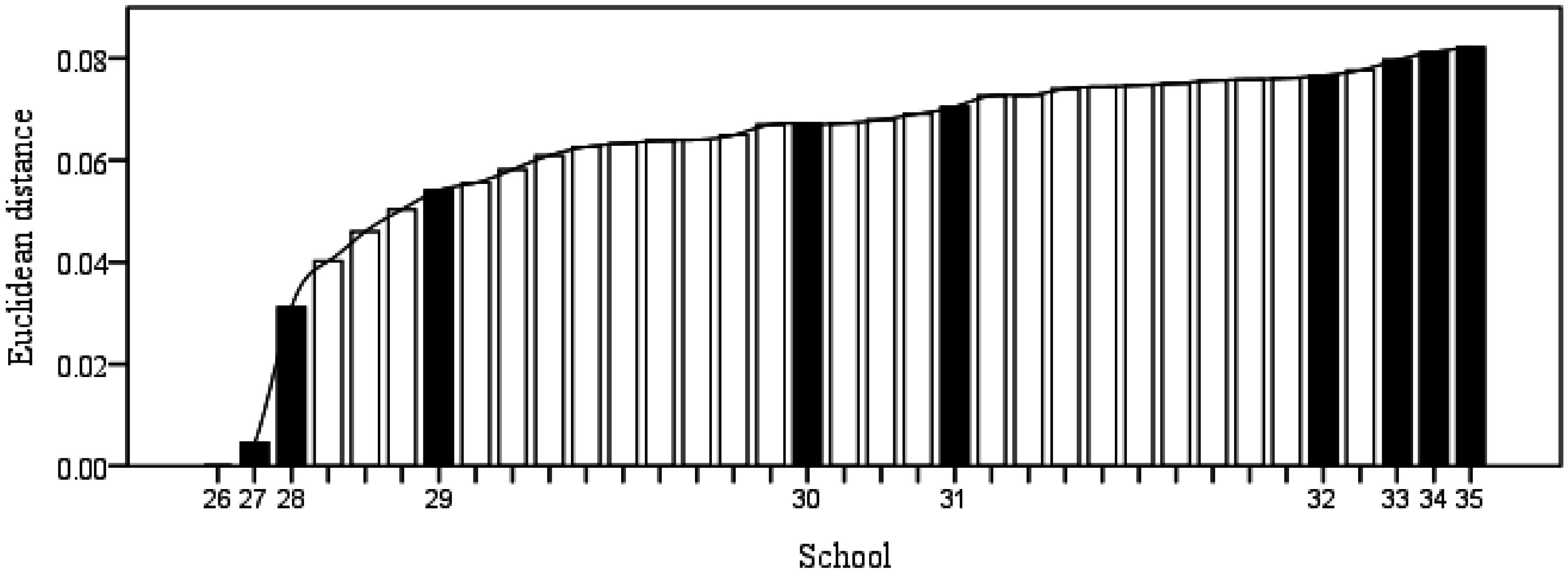
After solving Models (2) and (3), we can obtain the cross-efficiency matrix according to Models (4) and (5). After normalizing the elements in the cross-efficiency matrix, the final weights are calculated by using Model (12). Then, the relative Euclidean distances to the ideal cross-efficiency of all 35 DMUs can be calculated. These 35 schools are ranked according to the Euclidean distance results, which are shown in Figure 1. From Figure 1, we can find: (1) the Euclidean distance of DMU₂₆ is zero, so it should be ranked first among all DMUs; (2) DMU₃₅ has the largest Euclidean distance of 0.0822, so it is ranked last; (3) and the Euclidean distances gradually increase from DMU₂₆ to DMU₃₅. This indicates that performance rankings are gradually reduced from DMU₂₆ to DMU₃₅. These ranking results meet all the above observations, suggesting that the ranking obtained by our approach can represent the true ranking.

6. Conclusions

Traditional cross-efficiency models assume that the data of all DMUs are precise. However, this assumption is not always correct in the real world. In many real circumstances, the outputs and inputs of DMUs are not perfectly precise, which may only have a range in an interval form. In these cases, traditional cross-efficiency models cannot evaluate the efficiencies of DMUs. To address this problem, the present study proposes a new approach. In this approach, we firstly extend traditional cross-efficiency models for obtaining the interval efficiency of each DMU. Then, the distance entropy model is utilized to calculate the weights of interval cross-efficiency scores. Finally, all DMUs are assessed and ranked by the distance to the positive ideal cross-efficiency. A demonstrative case using data from China’s primary schools is used to illustrate the newly proposed model. Through this real case, we can conclude that the proposed method is convenient to solve problems with interval data of DMUs, and can provide complete and fair results for all DMUs.

The method proposed in this paper can be further expanded in the future studies. The DEA Shannon entropy model is proposed based on the cross-efficiency method. The proposed model can also be extended to other DEA models with intervals in the future studies. In addition, our study collected the imprecise data in an interval form. However, in some real cases, a proportion of data are missing. Under this circumstance, it is difficult to extend our method to evaluate the DMUs with missing data, but this direction is worth further investigation.

References

- Charnes, A.; Cooper, W.W.; Rhodes, E. Measuring the efficiency of decision making units. Eur. J. Oper. Res. 1978, 2, 429–444. [Google Scholar] [CrossRef]
- Co, H.C.; Chew, K.S. Performance and R&D expenditures in American and Japanese manufacturing firms. Int. J. Prod. Res. 1997, 35, 3333–3348. [Google Scholar]
- Johns, N.; Howcroft, B.; Drake, L. The use of data envelopment analysis to monitor hotel productivity. Progress in tourism and hospitality research. Prog. Tour. Hosp. Res. 1997, 3, 119–127. [Google Scholar] [CrossRef]
- Braglia, M.; Petroni, A. Evaluating and selecting investments in industrial robots. Int. J. Prod. Res. 1999, 37, 4157–4178. [Google Scholar] [CrossRef]
- Sun, S. Assessing computer numerical control machines using data envelopment analysis. Int. J. Prod. Res. 2002, 40, 2011–2039. [Google Scholar] [CrossRef]
- Reichmann, G.; Sommersguter-Reichmann, M. University library benchmarking: An international comparison using DEA. Int. J. Prod. Econ. 2006, 100, 131–147. [Google Scholar] [CrossRef]
- Wang, R.T.; Ho, C.T.B.; Oh, K. Measuring production and marketing efficiency using grey relation analysis and data envelopment analysis. Int. J. Prod. Res. 2010, 48, 183–199. [Google Scholar] [CrossRef]
- Sinuany-Stern, Z.; Mehrez, A.; Hadad, Y. An AHP/DEA methodology for ranking decision making units. Int. Trans. Oper. Res. 2000, 7, 109–124. [Google Scholar] [CrossRef]
- Sexton, T.R.; Silkman, R.H.; Hogan, A.J. Dataenvelopment analysis: Critique and extensions. New Dir. Eval. 1986, 73–105. [Google Scholar] [CrossRef]
- Doyle, J.; Green, R. Efficiency and cross-efficiency in DEA: Derivations, meanings and uses. J. Oper. Res. Soc. 1994, 45, 567–578. [Google Scholar] [CrossRef]
- Anderson, T.R.; Hollingsworth, K.; Inman, L. The fixed weighting nature of a cross-evaluation model. J. Prod. Anal. 2002, 17, 249–255. [Google Scholar] [CrossRef]
- Wu, J.; Liang, L.; Chen, Y. DEA game cross-efficiency approach to Olympic rankings. Omega 2009, 37, 909–918. [Google Scholar] [CrossRef]
- Falagario, M.; Sciancalepore, F.; Costantino, N.; Pietroforte, R. Using a DEA-cross efficiency approach in public procurement tenders. Eur. J. Oper. Res. 2012, 218, 523–529. [Google Scholar] [CrossRef]
- Lim, S.; Oh, K.W.; Zhu, J. Use of DEA cross-efficiency evaluation in portfolio selection: An application to Korean stock market. Eur. J. Oper. Res. 2014, 236, 361–368. [Google Scholar] [CrossRef]
- Cui, Q.; Li, Y. Evaluating energy efficiency for airlines: An application of VFB-DEA. J. Air Transp. Manag. 2015, 44–45, 34–41. [Google Scholar] [CrossRef]
- Despotis, D.K. Improving the discriminating power of DEA: Focus on globally efficient units. J. Oper. Res. Soc. 2002, 53, 314–323. [Google Scholar] [CrossRef]
- Liang, L.; Wu, J.; Cook, W.D.; Zhu, J. Alternative secondary goals in DEA cross-efficiency evaluation. Int. J. Prod. Econ. 2008, 113, 1025–1030. [Google Scholar] [CrossRef]
- Wang, Y.-M.; Chin, K.-S. Some alternative models for DEA cross-efficiency evaluation. Int. J. Prod. Econ. 2010, 128, 332–338. [Google Scholar] [CrossRef]
- Jahanshahloo, G.R.; Lotfi, F.H.; Jafari, Y.; Maddahi, R. Selecting symmetric weights as a secondary goal in DEA cross-efficiency evaluation. Appl. Math. Model. 2011, 35, 544–549. [Google Scholar] [CrossRef]
- Wu, J.; Sun, J.; Zha, Y.; Liang, L. Ranking approach of cross-efficiency based on improved TOPSIS technique. J. Syst. Eng. Electron. 2011, 22, 604–608. [Google Scholar] [CrossRef]
- Contreras, I. Optimizing the rank position of the DMU as secondary goal in DEA cross-evaluation. Appl. Math. Model. 2012, 36, 2642–2648. [Google Scholar] [CrossRef]
- Lim, S. Minimax and maximin formulations of cross-efficiency in DEA. Comput. Ind. Eng. 2012, 62, 726–731. [Google Scholar] [CrossRef]
- Maddahi, R.; Jahanshahloo, G.R.; Lotfi, H.F.; Ebrahimnejad, A. Optimising proportional weights as a secondary goal in DEA cross-efficiency evaluation. Int. J. Oper. Res. 2014, 19, 234–245. [Google Scholar] [CrossRef]
- Cook, W.D.; Zhu, J. DEA Cobb–Douglas frontier and cross-efficiency. J. Oper. Res. Soc. 2014, 65, 265–268. [Google Scholar] [CrossRef]
- Wu, J.; Chu, J.; Sun, J.; Zhu, Q. DEA cross-efficiency evaluation based on Pareto improvement. Eur. J. Oper. Res. 2016, 248, 571–579. [Google Scholar] [CrossRef]
- Wu, J.; Liang, L.; Yang, F. Determination of the weights for the ultimate cross efficiency using Shapley value in cooperative game. Expert Syst. Appl. 2009, 36, 872–876. [Google Scholar] [CrossRef]
- Wang, Y.M.; Wang, S. Approaches to determining the relative importance weights for cross-efficiency aggregation in data envelopment analysis. J. Oper. Res. Soc. 2013, 64, 60–69. [Google Scholar] [CrossRef]
- Angiz, M.Z.; Mustafa, A.; Kamali, M.J. Cross-ranking of decision making units in data envelopment analysis. Appl. Math. Model. 2013, 37, 398–405. [Google Scholar] [CrossRef]
- Yang, G.-L.; Yang, J.-B.; Liu, W.-B.; Li, X.-X. Cross-efficiency aggregation in DEA models using the evidential-reasoning approach. Eur. J. Oper. Res. 2013, 231, 393–404. [Google Scholar] [CrossRef]
- Cooper, W.W.; Park, K.S.; Yu, G. An illustrative application of IDEA (imprecise data envelopment analysis) to a Korean mobile telecommunication company. Oper. Res. 2001, 49, 807–820. [Google Scholar] [CrossRef]
- Lee, Y.K.; Park, K.S.; Kim, S.H. Identification of inefficiencies in an additive model based IDEA (imprecise data envelopment analysis). Comput. Oper. Res. 2002, 29, 1661–1676. [Google Scholar] [CrossRef]
- Despotis, D.K.; Smirlis, Y.G. Data envelopment analysis with imprecise data. Eur. J. Oper. Res. 2002, 140, 24–36. [Google Scholar] [CrossRef]
- Wang, Y.-M.; Greatbanks, R.; Yang, J.-B. Interval efficiency assessment using data envelopment analysis. Fuzzy Sets Syst. 2005, 153, 347–370. [Google Scholar] [CrossRef]
- Azizi, H.; Jahed, R. An improvement for efficiency interval: Efficient and inefficient frontiers. Int. J. Appl. Oper. Res. 2011, 1, 49–63. [Google Scholar]
- Wang, Y.-M.; Chin, K.-S. Fuzzy data envelopment analysis: A fuzzy expected value approach. Expert Syst. Appl. 2011, 38, 11678–11685. [Google Scholar] [CrossRef]
- Dotoli, M.; Epicoco, N.; Falagario, M.; Sciancalepore, F. A cross-efficiency fuzzy Data Envelopment Analysis technique for the performance evaluation of Decision Making Units under uncertainty. Comput. Ind. Eng. 2015, 79, 103–114. [Google Scholar] [CrossRef]
- Wang, Y.-M.; Chin, K.-S. A neutral DEA model for cross-efficiency evaluation and its extension. Expert Syst. Appl. 2010, 37, 3666–3675. [Google Scholar] [CrossRef]
- Oukil, A.; Amin, G.R. Maximum appreciative cross-efficiency in DEA: A new ranking method. Comput. Ind. Eng. 2015, 81, 14–21. [Google Scholar] [CrossRef]
- Cook, W.D.; Zhu, J. DEA Cross Efficiency. In Data Envelopment Analysis: A Handbook of Models and Methods; Zhu, J., Ed.; Springer: Berlin/Heidelberg, Germany, 2015; pp. 23–43. [Google Scholar]
- Lim, S.; Zhu, J. DEA Cross efficiency under variable returns to scale. In Data Envelopment Analysis: A Handbook of Models and Methods; Zhu, J., Ed.; Springer: Berlin/ Heidelberg, Germany, 2015; pp. 45–66. [Google Scholar]
- Cooper, W.W.; Seiford, L.M.; Zhu, J. Data envelopment analysis: History, models, and interpretations. In Handbook on Data Envelopment Analysis; Springer: Berlin/ Heidelberg, Germany, 2004; pp. 1–39. [Google Scholar]
- Cook, W.D.; Bala, K. Performance measurement and classification data in DEA: Input-oriented model. Omega 2007, 35, 39–52. [Google Scholar] [CrossRef]
- Shannon, C.E. The mathematical theory of communication. Bell Syst. Tech. J. 1948, 27, 379–423, 623–656. [Google Scholar] [CrossRef]
- Lo Storto, C. Ecological Efficiency Based Ranking of Cities: A Combined DEA Cross-Efficiency and Shannon’s Entropy Method. Sustainability 2016, 8, 124. [Google Scholar] [CrossRef]
- Xie, Q.; Dai, Q.; Li, Y.; Jiang, A. Increasing the discriminatory power of DEA using Shannon’s entropy. Entropy 2014, 16, 1571–1585. [Google Scholar] [CrossRef]
- Qi, X.-G.; Guo, B. Determining common weights in data envelopment analysis with Shannon’s entropy. Entropy 2014, 16, 6394–6414. [Google Scholar] [CrossRef]
- Wang, Y.-M.; Parkan, C. A general multiple attribute decision-making approach for integrating subjective preferences and objective information. Fuzzy Sets Syst. 2006, 157, 1333–1345. [Google Scholar] [CrossRef]
- Wang, Y.-M.; Luo, Y. Integration of correlations with standard deviations for determining attribute weights in multiple attribute decision making. Math. Comput. Model. 2010, 51, 1–12. [Google Scholar] [CrossRef]
- Tzeng, G.H.; Huang, J.J. Multiple Attribute Decision Making: Methods and Applications; CRC Press: Boca Raton, FL, USA, 2011; p. 349. [Google Scholar]
- Sun, J.; Miao, Y.; Wu, J.; Cui, L.; Zhong, R. Improved interval DEA models with common weight. Kybernetika 2014, 50, 774–785. [Google Scholar] [CrossRef]
- Hadad, Y.; Hanani, M.Z. Combining the AHP and DEA methodologies for selecting the best alternative. Int. J. Logist. Syst. Manag. 2011, 9, 251–267. [Google Scholar] [CrossRef]
- Ganley, J.A.; Cubbin, S.J. Public Sector Efficiency Measurement: Applications of Data Envelopment Analysis; Elsevier: Amsterdam, The Netherlands, 1992. [Google Scholar]
- Friedman, L.; Sinuany-Stern, Z. Combining ranking scales and selecting variables in the DEA context. The case of industrial branches. Comput. Oper. Res. 1998, 25, 781–791. [Google Scholar] [CrossRef]
- Adler, N.; Friedman, L.; Sinuany-Stern, Z. Review of ranking methods in the DEA context. Eur. J. Oper. Res. 2002, 140, 249–265. [Google Scholar] [CrossRef]
- Wang, Y.M.; Chin, K.S.; Jiang, P. Weight determination in the cross-efficiency evaluation. Comput. Ind. Eng. 2011, 61, 497–502. [Google Scholar] [CrossRef]
- Ramón, N.; Ruiz, J.L.; Sirvent, I. Reducing differences between profiles of weights: A “peer-restricted” cross-efficiency evaluation. Omega 2011, 39, 634–641. [Google Scholar] [CrossRef]
Figure 1.
The Euclidean distances of 35 DMUs.