The Analytical Solution of Parabolic Volterra Integro-Differential Equations in the Infinite Domain

Abstract

This article focuses on obtaining analytical solutions for d-dimensional, parabolic Volterra integro-differential equations with different types of frictional memory kernel. Based on Laplace transform and Fourier transform theories, the properties of the Fox-H function and convolution theorem, analytical solutions for the equations in the infinite domain are derived under three frictional memory kernel functions. The analytical solutions are expressed by infinite series, the generalized multi-parameter Mittag-Leffler function, the Fox-H function and the convolution form of the Fourier transform. In addition, graphical representations of the analytical solution under different parameters are given for one-dimensional parabolic Volterra integro-differential equations with a power-law memory kernel. It can be seen that the solution curves are subject to Gaussian decay at any given moment.

1. Introduction

In this paper, we will consider the following high (d-) dimensional parabolic Volterra integro-differential equation with memory kernel $\mathcal{K}(t)$ in the infinite domain [1]:

$$\frac{\partial u(x,t)}{\partial t}+{\displaystyle {\int }_0^t\mathcal{K}(t-t^{\prime })}u(x,t^{\prime })\mathrm{d}{t}^{\prime }=\Delta u(x,t)+f(x,t),$$

(1)

which satisfies the initial condition and boundary conditions below,

$$u(x,0)=g(x),\underset{\left|x\right|\to \infty }{\lim }u(x,t)=0,t>0,x=(x_1,x_2,\cdot \cdot \cdot ,x_d)\in R^d.$$

(2)

where function $f(x,t)$ and memory kernel function $\mathcal{K}(t)$ are assumed to be sufficiently smooth functions, and $\Delta$ is the d-dimensional Laplacian operator.

Parabolic Volterra integro-differential equations present an important model to simulate the effects of the “memory” of the system. The model is based on a partial differential equation, combining the partial differentiation and integral term containing the unknown kernel function that leads to parabolic Volterra integro-differential equations. In general, the model nonlocal effects of the memory of past history cannot be described by partial differential equations. Therefore, more and more researchers have studied the solution of integro-differential equations.

Diffusion is one of the most important and ubiquitous phenomena in nature. The parabolic Volterra integro-differential equation model Equation (1) can be also describe anomalous diffusion; see references [2,3]. The reaction diffusion level most depends on the choice of the kernel $\mathcal{K}(t)$ present in the nonlocal reaction diffusion (integral) term.

Parabolic Volterra integro-differential equations have many important physical applications to model dynamical systems, such as in compression of viscoelastic media [4], nuclear reactor dynamics [5], blow-up problems [6], reaction diffusion problems [7] and heat conduction materials with memory functional [8], etc. So far, the analysis of numerical solution of Volterra integral-differential equations has been carried out by many authors. Avazzadeh et al. [9] proposed radial basis functions through the finite difference method to find a nonlinear Volterra integro-differential equation’s numerical solution. Aguilar et al. [10] proposed collocation methods to solve second-order parabolic Volterra integro-differential equations. Dehghan et al. [8] studied numerical solution of parabolic integro-differential equations using the variational iteration method. Han et al. [1] proposed the artificial boundary method to solve parabolic Volterra integro differential equations (one/two-dimensional) in infinite spatial domains. Fakhar-Izadi et al. [11] considered the parabolic Volterra integro-differential equation in one-dimensional finite and infinite spatial domains using spectral collocation methods. Vasudeva Murthy et al. [12] investigated parabolic integro-differential equations through explicit integration and the Runge-Kutta-Chebyshev method.

However, to the authors’ knowledge, there are no studies on analytical solutions of parabolic partial Volterra integro-differential equation in the infinite domain. In this article, our goal is mainly to discuss analytical solutions of Equation (1) with three different kinds of memory kernel functions in the infinite domain.

This paper is organized as follows. In Section 2, some definitions and lemmas are introduced. In Section 3, the analytical solutions of parabolic Volterra integro-differential equation with three different kinds of memory kernel are demonstrated in the infinite domain. In Section 4, a typical example and some graphical representations of the solution are presented. Some conclusions are given in Section 5.

2. Preliminaries

In this section, we present some fundamental definitions and lemmas that are used throughout this paper.

Definition 1.

A four-parameter Mittag-Leffler (M-L) function is defined as [13]

$$E_{\alpha ,\beta }^{\gamma ,\kappa }(z):={\displaystyle \sum _{n=0}^{\infty }\frac{{(\gamma )}_{n\kappa }}{\mathrm{\Gamma }(\alpha n+\beta )}}\cdot \frac{z^n}{n!},$$

(3)

where $z,\beta ,\gamma ,\kappa \in \mathrm{ℂ}$, $\mathrm{\Re }(\alpha )>$ max $\left(\left\{0,\mathrm{\Re }(\kappa )-1\right\},\mathrm{\Re }(\kappa )>0\right)$, with Pochammer’s symbol ${(\gamma )}_{n\kappa }$ can be expressed as

$${(\gamma )}_{n\kappa }:=\mathrm{\Gamma }(\gamma +n\kappa )/\mathrm{\Gamma }(\gamma )=\{\begin{array}{l}1,ifn\kappa =0\\ \gamma (\gamma +1)(\gamma +2)\mathrm{...}(\gamma +n\kappa -1),ifn\kappa \in N,\gamma \ne 0\end{array}.$$

It is worth noting that when $\kappa =1$, the three-parameter Mittag-Leffler function can be expressed as $E_{\alpha ,\beta }^{\gamma ,1}(\cdot )=E_{\alpha ,\beta }^{\gamma }(\cdot )$ [13,14]:

$$E_{\alpha ,\beta }^{\gamma }(z):={\displaystyle \sum _{n=0}^{\infty }\frac{{(\gamma )}_n}{\mathrm{\Gamma }(\alpha n+\beta )}}\cdot \frac{z^n}{n!},$$

(4)

where $\alpha ,\beta ,\gamma \in \mathrm{ℂ}$, and ${(\gamma )}_n$ is the Pochhammer symbol.

Note the relation between generalized the Mittag-Leffler function and the Fox-H function:

$$E_{\alpha ,\beta }^{\gamma }(z)=\frac{1}{\mathrm{\Gamma }(\gamma )}{H}_{1,2}^{1,1}\left[-z|\begin{array}{cc}(1-\gamma ,1)& \\ (0,1),& (1-\beta ,\alpha )\end{array}\right].$$

where $H_{1,2}^{1,1}(z)$ [15] is a Fox-H function, and $(\mathrm{\Re }(\alpha ),\mathrm{\Re }(\beta ),\mathrm{\Re }(\gamma )>0)$.

Note that, when $\gamma =1$, we can obtain a two-parameter Mittag-Leffler function $E_{\alpha ,\beta }^1(\cdot )=E_{\alpha ,\beta }(\cdot )$ [16], there

$$E_{\alpha ,\beta }(z):={\displaystyle \sum _{n=0}^{\infty }\frac{z^n}{\mathrm{\Gamma }(\alpha n+\beta )}},$$

(5)

where $z,\beta \in \mathrm{ℂ}$, $\mathrm{\Re }(\alpha )>0$. Note that $E_{\alpha ,1}(\cdot )$ reduces to Mittag-Leffler function $E_{\alpha }(\cdot )$ when $\beta =1$, then

$$E_{\alpha ,1}(z)=E_{\alpha }(z):={\displaystyle \sum _{n=0}^{\infty }\frac{z^n}{\mathrm{\Gamma }(\alpha n+1)}},$$

where $z\in \mathrm{ℂ}$, $\mathrm{\Re }(\alpha )>0$. In particular, we can obtain a regular exponential function when $\alpha =1$.

Definition 2.

An integral operator ${ℰ}_{a+;\alpha ,\beta }^{w;\gamma ,\kappa }\phi$ is defined as [17,18]

$$\left({ℰ}_{a+;\alpha ,\beta }^{w;\gamma ,\kappa }\phi \right)(t):=\left(t^{\beta -1}{E}_{\alpha ,\beta }^{\gamma ,\kappa }(w{t}^{\alpha })\right)\ast \phi (t)={\displaystyle {\int }_a^t{(t-\tau )}^{\beta -1}}{E}_{\alpha ,\beta }^{\gamma ,\kappa }(w{(t-\tau )}^{\alpha })\phi (\tau )\mathrm{d}\tau .$$

(6)

It is worth noting that, when $w=0$ and $a=0$, integral operator ${ℰ}_{a+;\alpha ,\beta }^{w;\gamma ,\kappa }\phi$ would correspond to the Riemann-Liouville integral operator [13].

In this section, we will introduce some fundamental lemmas for the Laplace transform ($ℒ$), which will be help us handle some problems in the next section.

Lemma 1.

Let s, b, α, ${\lambda }_n\in {\mathrm{ℝ}}^{+}$, and then the following inverse Laplace transform (${ℒ}^{-1}$) is true [18].

$${ℒ}^{-1}\left\{\frac{1}{s^2+b{s}^{\alpha }+{\lambda }_n}ℒ\left[g(t)\right](s)\right\}(t)={\displaystyle \sum _{n=0}^{\infty }{(-b)}^n}\left({ℰ}_{0+;2,(2-\alpha )(n+1)+1}^{-{\lambda }_n;n+1,1}g\right)(t),$$

(7)

where

$$0<\frac{{\lambda }_n}{s^2+b{s}^{\alpha }}<1,0<\frac{b}{s^{2-\alpha }}<1.$$

Lemma 2.

The Laplace transform of a three-parameter Mittag-Leffler function is given by [18,19]

$$ℒ\left[t^{\beta -1}{E}_{\alpha ,\beta }^{\gamma }(\pm w{t}^{\alpha })\right](s)={\displaystyle {\int }_0^{\infty }{e}^{-st}}{t}^{\beta -1}{E}_{\alpha ,\beta }^{\gamma }(\pm w{t}^{\alpha })\mathrm{d}t=\frac{s^{\alpha \gamma -\beta }}{{(s^{\alpha }\mp w)}^{\gamma }},$$

(8)

where $\left|w/s^{\alpha }\right|<1$.

Lemma 3.

The Laplace transform of $e^{-\lambda t}{t}^{\beta -1}{E}_{\alpha ,\beta }^{\gamma }(w{t}^{\alpha })$ is given by the following [19]:

$$ℒ\left[e^{-\lambda t}{t}^{\beta -1}{E}_{\alpha ,\beta }^{\gamma }(\pm w{t}^{\alpha })\right](s)=\frac{{(s+\lambda )}^{\alpha \gamma -\beta }}{{\left({(s+\lambda )}^{\alpha }\mp w\right)}^{\gamma }},(\lambda \ge 0)$$

(9)

where $\left|w/{(s+\lambda )}^{\alpha }\right|<1$.

It is worth noting that in case $\lambda =0$, the structure of Lemma 3 is equivalent to Lemma 2.

Lemma 4 gives one important d-dimensional integral formula for the Mittag-Leffler function.

Lemma 4.

For arbitrary α > 0, β is an arbitrary complex number, $\mu >0$, and $a\in R$, establishing the following formula: [20]

$${\displaystyle {\int }_{R^d}{e}^{ik\cdot x}{E}_{\alpha ,\beta }^{(n)}(-a{\left|k\right|}^{\mu }){\mathrm{d}}^{d}k={(2\pi )}^{d/2}{\left|x\right|}^{1-d/2}\times {\displaystyle {\int }_0^{\infty }{\left|k\right|}^{d/2}}{E}_{\alpha ,\beta }^{(n)}(-a{\left|k\right|}^{\mu })J_{d/2-1}(\left|x\right|\left|k\right|)}{\mathrm{d}}^d\left|k\right|.$$

(10)

In fact, here $J_{d/2-1}(\cdot )$ is a Bessel function, and $E_{\alpha ,\beta }^{(n)}(z)$ denotes the n-th derivatives of the two-parameter Mittag-Leffler function. n-th derivatives of the two-parameter Mittag-Leffler function can be expressed in terms of the Fox-H function as

$$E_{\alpha ,\beta }^{(n)}(z)=H_{1,2}^{1,1}\left[-z|\begin{array}{cc}(-n,1)& \\ (0,1),& (1-(\alpha n+\beta ),\alpha )\end{array}\right],$$

Furthermore, on the right of Equation (10) is the following:

$$\begin{gathered} {(\left|x\right|\left|k\right|)}^{1-d/2}{J}_{d/2-1}(\left|x\right|\left|k\right|)=2^{1-d/2}{H}_{0,2}^{1,0}\left[{\left(\frac{\left|x\right|\left|k\right|}{2}\right)}^2|\begin{array}{l}\\ (0,1)(1-d/2,1)\end{array}\right]. \\ k=(k_1,k_2,\cdot \cdot \cdot ,k_d)\in R^d \end{gathered}$$

where $H_{0,2}^{1,0}(z)$ [15] is the Fox-H function.

3. Analytical Solution of a Parabolic Volterra Integro-Differential Equation in the Infinite Domain

3.1. Analytical Solution with Frictional Memory Kernel of M-L type $\mathcal{K}(t)=\frac{1}{{\tau }^{\alpha \delta }}{t}^{\beta -1}{E}_{\alpha ,\beta }^{\delta }(-\frac{t^{\alpha }}{{\tau }^{\alpha }})$

In this case, Equation (1) can be written as follows:

$$\frac{\partial u(x,t)}{\partial t}+\frac{1}{{\tau }^{\alpha \delta }}{\displaystyle {\int }_0^t{(t-t^{\prime })}^{\beta -1}{E}_{\alpha ,\beta }^{\delta }(-\frac{{(t-t^{\prime })}^{\alpha }}{{\tau }^{\alpha }})}u(x,t^{\prime })\mathrm{d}t=\Delta u(x,t)+f(x,t).x\in R^d,t>0$$

(11)

where $\alpha ,\beta ,\delta >0$, $\tau$ is the memory time.

Theorem 1.

The analytical solution of parabolic Volterra integro-differential Equation (11) with boundary conditions and initial condition (2) can be expressed as the following analytical form

$$\begin{array}{c}u(x,t)=\frac{1}{{(2\pi )}^d}{\displaystyle {\int }_{R^d}{\displaystyle \sum _{i=0}^{\infty }{(-\frac{1}{{\tau }^{\alpha \delta }})}^i{\displaystyle \sum _{n=0}^i\left(\begin{array}{c}i\\ n\end{array}\right)}{(\frac{{\left|k\right|}^2}{1/{\tau }^{\alpha \delta }})}^n\left({ℰ}_{0+;\alpha ,(\beta +1)(i-n)+n+1}^{-{\tau }^{-\alpha };\delta (i-n),1}\tilde{f}\right)(k,t)e^{ik\cdot x}{\mathrm{d}}^{d}k}}\\ +{\displaystyle {\int }_{R^d}G(x-x^{\prime },t)g(x^{\prime }){\mathrm{d}}^d{x}^{\prime }}.x,k\in R^d\end{array}$$

(12)

In which $G(x,t)$ is the Green function and reads as

$$G(x,t)=\frac{1}{{(2\pi )}^d}{\displaystyle {\int }_{R^d}\left({\displaystyle \sum _{i=0}^{\infty }{(-\frac{1}{{\tau }^{\alpha \delta }})}^i{\displaystyle \sum _{n=0}^i\left(\begin{array}{c}i\\ n\end{array}\right)}{(\frac{{\left|k\right|}^2}{1/{\tau }^{\alpha \delta }})}^n{t}^{(\beta +1)(i-n)+n}{E}_{\alpha ,(\beta +1)(i-n)+n+1}^{\delta (i-n)}(-{\tau }^{-\alpha }{t}^{\alpha })}\right)}{e}^{ik\cdot x}{\mathrm{d}}^{d}k.$$

In general, this denotes $\tilde{f}(k,t)={\displaystyle {\int }_{R^d}{e}^{-ik\cdot x}}f(x,t){\mathrm{d}}^{d}x,(x\in R)$ as the Fourier transform of $f(x,t)$ with respect to the spatial variable $x$. The Laplace transform of a function $u(x,t)$ with regard to the time variable $t$ is defined as $\widehat{u}(k,t)={\displaystyle {\int }_0^{\infty }{e}^{-st}}u(k,t)\mathrm{d}t,(t>0).$

Proof. 

This denotes $ℱ\left\{u(x,t)\right\}:=\tilde{u}(k,t)$ as the Fourier transform of $u(x,t)$ with respect to variable $x$, and $ℒ\left\{u(x,t)\right\}:=\widehat{u}(x,s)$ as the Laplace transform of $u(x,t)$ with respect to variable $t$. Taking the Laplace transform with respect to the time variable t and the Fourier transform with respect to the spatial variable x to Equation (11), we obtain a nonhomogeneous equation, which can be written as the following:

$$s\widehat{\tilde{u}}(k,s)-\tilde{u}(k,0)+\frac{1}{{\tau }^{\alpha \delta }}\frac{s^{\alpha \delta -\beta }}{{(s^{\alpha }+{\tau }^{-\alpha })}^{\delta }}\widehat{\tilde{u}}(k,s)=-{\left|k\right|}^2\widehat{\tilde{u}}(k,s)+\widehat{\tilde{f}}(k,s).k\in R^d$$

(13)

Using the initial condition, it yields:

$$\widehat{\tilde{u}}(k,s)=\frac{1}{s+\frac{1}{{\tau }^{\alpha \delta }}\frac{s^{\alpha \delta -\beta }}{{(s^{\alpha }+{\tau }^{-\alpha })}^{\delta }}+{\left|k\right|}^2}\widehat{\tilde{f}}(k,s)+\frac{1}{s+\frac{1}{{\tau }^{\alpha \delta }}\frac{s^{\alpha \delta -\beta }}{{(s^{\alpha }+{\tau }^{-\alpha })}^{\delta }}+{\left|k\right|}^2}\tilde{g}(k).$$

(14)

Because

$$\begin{array}{c}\frac{1}{s+\frac{1}{{\tau }^{\alpha \delta }}\frac{s^{\alpha \delta -\beta }}{{(s^{\alpha }+{\tau }^{-\alpha })}^{\delta }}+{\left|k\right|}^2}=s^{-1}{\displaystyle \sum _{i=0}^{\infty }{(-\frac{1}{{\tau }^{\alpha \delta }})}^i}{\displaystyle \sum _{n=0}^i\left(\begin{array}{c}i\\ n\end{array}\right)}{({\left|k\right|}^2{s}^{-1})}^n{(\frac{s^{\alpha \delta -\beta -1}}{{(s^{\alpha }+{\tau }^{-\alpha })}^{\delta }})}^{i-n}{(\frac{1}{{\tau }^{\alpha \delta }})}^{-n}\\ ={\displaystyle \sum _{i=0}^{\infty }{(-\frac{1}{{\tau }^{\alpha \delta }})}^i}{\displaystyle \sum _{n=0}^i\left(\begin{array}{c}i\\ n\end{array}\right)}\frac{s^{\alpha \delta (i-n)-(\beta +1)(i-n)-n-1}}{{(s^{\alpha }+{\tau }^{-\alpha })}^{\delta (i-n)}}{(\frac{{\left|k\right|}^2}{1/{\tau }^{\alpha \delta }})}^n,\end{array}$$

(15)

Employing Lemma 2, we can get

$$\frac{s^{\alpha \delta (i-n)-(\beta +1)(i-n)-n-1}}{{(s^{\alpha }+{\tau }^{-\alpha })}^{\delta (i-n)}}=ℒ\left[t^{(\beta +1)(i-n)+n}{E}_{\alpha ,(\beta +1)(i-n)+n+1}^{\delta (i-n)}(-{\tau }^{-\alpha }{t}^{\alpha })\right](s).$$

(16)

Substituting Equations (15) and (16) into the first term of Equation (14), we have

$$\begin{array}{c}\frac{1}{s+\frac{1}{{\tau }^{\alpha \delta }}\frac{s^{\alpha \delta -\beta }}{{(s^{\alpha }+{\tau }^{-\alpha })}^{\delta }}+{\left|k\right|}^2}\widehat{\tilde{f}}(k,s)=\\ ℒ\left[{\displaystyle \sum _{i=0}^{\infty }{(-\frac{1}{{\tau }^{\alpha \delta }})}^i}{\displaystyle \sum _{n=0}^i\left(\begin{array}{c}i\\ n\end{array}\right)}{(\frac{{\left|k\right|}^2}{1/{\tau }^{\alpha \delta }})}^n{t}^{(\beta +1)(i-n)+n}{E}_{\alpha ,(\beta +1)(i-n)+n+1}^{\delta (i-n)}(-{\tau }^{-\alpha }{t}^{\alpha })\right](s)ℒ\left[\tilde{f}(k,t)\right](s).\end{array}$$

(17)

By applying inverse Laplace transform (${ℒ}^{-1}$), the convolution definition of a Laplace transform and Definition 2, we can obtain the inverse Laplace transform of the first term in Equation (14) as follows:

$$\begin{array}{c}{ℒ}^{-1}\left(\frac{1}{s+\frac{1}{{\tau }^{\alpha \delta }}\frac{s^{\alpha \delta -\beta }}{{(s^{\alpha }+{\tau }^{-\alpha })}^{\delta }}+{\left|k\right|}^2}ℒ\left(\tilde{f}(k,t)\right)(s)\right)(t)=\\ {\displaystyle \sum _{i=0}^{\infty }{(-\frac{1}{{\tau }^{\alpha \delta }})}^i}{\displaystyle \sum _{n=0}^i\left(\begin{array}{c}i\\ n\end{array}\right)}{(\frac{{\left|k\right|}^2}{1/{\tau }^{\alpha \delta }})}^n\left({ℰ}_{0+;\alpha ,(\beta +1)(i-n)+n+1}^{-{\tau }^{-\alpha };\delta (i-n),1}\tilde{f}\right)(k,t).\end{array}$$

(18)

It follows that the inverse Laplace transform of the second term in Equation (14) is

$$\begin{array}{c}{ℒ}^{-1}\left(\frac{1}{s+\frac{1}{{\tau }^{\alpha \delta }}\frac{s^{\alpha \delta -\beta }}{{(s^{\alpha }+{\tau }^{-\alpha })}^{\delta }}+{\left|k\right|}^2}\tilde{g}(k)\right)(t)=\\ {\displaystyle \sum _{i=0}^{\infty }{(-\frac{1}{{\tau }^{\alpha \delta }})}^i}{\displaystyle \sum _{n=0}^i\left(\begin{array}{c}i\\ n\end{array}\right)}{(\frac{{\left|k\right|}^2}{1/{\tau }^{\alpha \delta }})}^n{t}^{(\beta +1)(i-n)+n}{E}_{\alpha ,(\beta +1)(i-n)+n+1}^{\delta (i-n)}(-{\tau }^{-\alpha }{t}^{\alpha })\tilde{g}(k).\end{array}$$

(19)

According to Equations (18) and (19), we can obtain $\tilde{u}(k,t)$ from Equation (14)

$$\begin{array}{c}\tilde{u}(k,t)={\displaystyle \sum _{i=0}^{\infty }{(-\frac{1}{{\tau }^{\alpha \delta }})}^i}{\displaystyle \sum _{n=0}^i\left(\begin{array}{c}i\\ n\end{array}\right)}{(\frac{{\left|k\right|}^2}{1/{\tau }^{\alpha \delta }})}^n\left({ℰ}_{0+;\alpha ,(\beta +1)(i-n)+n+1}^{-{\tau }^{-\alpha };\delta (i-n),1}\tilde{f}\right)(k,t)+\\ {\displaystyle \sum _{i=0}^{\infty }{(-\frac{1}{{\tau }^{\alpha \delta }})}^i}{\displaystyle \sum _{n=0}^i\left(\begin{array}{c}i\\ n\end{array}\right)}{(\frac{{\left|k\right|}^2}{1/{\tau }^{\alpha \delta }})}^n{t}^{(\beta +1)(i-n)+n}{E}_{\alpha ,(\beta +1)(i-n)+n+1}^{\delta (i-n)}(-{\tau }^{-\alpha }{t}^{\alpha })\tilde{g}(k).\end{array}$$

(20)

Equation (20) can be further manipulated by employing an inverse Fourier transform:

$$\begin{array}{c}u(x,t)=\frac{1}{{(2\pi )}^d}{\displaystyle {\int }_{R^d}{e}^{ik\cdot x}{\displaystyle \sum _{i=0}^{\infty }{(-\frac{1}{{\tau }^{\alpha \delta }})}^i}{\displaystyle \sum _{n=0}^i\left(\begin{array}{c}i\\ n\end{array}\right)}{(\frac{{\left|k\right|}^2}{1/{\tau }^{\alpha \delta }})}^n\left({ℰ}_{0+;\alpha ,(\beta +1)(i-n)+n+1}^{-{\tau }^{-\alpha };\delta (i-n),1}\tilde{f}\right)(k,t){\mathrm{d}}^{d}k}+\\ \frac{1}{{(2\pi )}^d}{\displaystyle {\int }_{R^d}{e}^{ik\cdot x}{\displaystyle \sum _{i=0}^{\infty }{(-\frac{1}{{\tau }^{\alpha \delta }})}^i}{\displaystyle \sum _{n=0}^i\left(\begin{array}{c}i\\ n\end{array}\right)}{(\frac{{\left|k\right|}^2}{1/{\tau }^{\alpha \delta }})}^n{t}^{(\beta +1)(i-n)+n}{E}_{\alpha ,(\beta +1)(i-n)+n+1}^{\delta (i-n)}(-{\tau }^{-\alpha }{t}^{\alpha })\tilde{g}(k){\mathrm{d}}^{d}k}.\end{array}$$

(21)

We need $\left|\frac{1}{{\tau }^{\alpha \delta }}\frac{s^{\alpha \delta -\beta -1}}{{(s^{\alpha }+{\tau }^{-\alpha })}^{\delta }}+{\left|k\right|}^2{s}^{-1}\right|<1,$ and we presented that the series and integrals (21) are convergent. And $E_{\alpha ,(\beta +1)(i-n)+n+1}^{\delta (i-n)}(\cdot )$ is generalization of the Mittag-Leffler function.

The second term in Equation (21) can be further manipulated as follows

$$\begin{array}{c}\frac{1}{{(2\pi )}^d}{\displaystyle {\int }_{R^d}{e}^{ik\cdot x}{\displaystyle \sum _{i=0}^{\infty }{(-\frac{1}{{\tau }^{\alpha \delta }})}^i}{\displaystyle \sum _{n=0}^i\left(\begin{array}{c}i\\ n\end{array}\right)}{(\frac{{\left|k\right|}^2}{1/{\tau }^{\alpha \delta }})}^n{t}^{(\beta +1)(i-n)+n}{E}_{\alpha ,(\beta +1)(i-n)+n+1}^{\delta (i-n)}(-{\tau }^{-\alpha }{t}^{\alpha })\tilde{g}(k){\mathrm{d}}^{d}k}\\ =\frac{1}{{(2\pi )}^d}{\displaystyle {\int }_{R^d}{e}^{ik\cdot x}{\displaystyle \sum _{i=0}^{\infty }{(-\frac{1}{{\tau }^{\alpha \delta }})}^i}{\displaystyle \sum _{n=0}^i\left(\begin{array}{c}i\\ n\end{array}\right)}{(\frac{{\left|k\right|}^2}{1/{\tau }^{\alpha \delta }})}^n{t}^{(\beta +1)(i-n)+n}{E}_{\alpha ,(\beta +1)(i-n)+n+1}^{\delta (i-n)}(-{\tau }^{-\alpha }{t}^{\alpha })\left({\displaystyle {\int }_{R^d}{e}^{-ik\cdot x^{\prime }}g(x^{\prime }){\mathrm{d}}^d{x}^{\prime }}\right)}{\mathrm{d}}^{d}k\\ ={\displaystyle {\int }_{R^d}\left[\frac{1}{{(2\pi )}^d}{\displaystyle {\int }_{R^d}{e}^{ik\cdot (x-x^{\prime })}{\displaystyle \sum _{i=0}^{\infty }{(-\frac{1}{{\tau }^{\alpha \delta }})}^i}{\displaystyle \sum _{n=0}^i\left(\begin{array}{c}i\\ n\end{array}\right)}{(\frac{{\left|k\right|}^2}{1/{\tau }^{\alpha \delta }})}^n{t}^{(\beta +1)(i-n)+n}{E}_{\alpha ,(\beta +1)(i-n)+n+1}^{\delta (i-n)}(-{\tau }^{-\alpha }{t}^{\alpha }){\mathrm{d}}^{d}k}\right]}g(x^{\prime }){\mathrm{d}}^d{x}^{\prime }. \end{array}$$

(22)

Denote Green function $G(x,t)$ is

$$G(x-x^{\prime },t)=\frac{1}{{(2\pi )}^d}{\displaystyle {\int }_{R^d}{e}^{ik\cdot (x-x^{\prime })}{\displaystyle \sum _{i=0}^{\infty }{(-\frac{1}{{\tau }^{\alpha \delta }})}^i}{\displaystyle \sum _{n=0}^i\left(\begin{array}{c}i\\ n\end{array}\right)}{(\frac{{\left|k\right|}^2}{1/{\tau }^{\alpha \delta }})}^n{t}^{(\beta +1)(i-n)+n}{E}_{\alpha ,(\beta +1)(i-n)+n+1}^{\delta (i-n)}(-{\tau }^{-\alpha }{t}^{\alpha }){\mathrm{d}}^{d}k}.$$

Therefore, we complete the proof of Theorem 1. □

3.2. Analytical Solution with a Frictional Memory Kernel of Power-Law Type $\mathcal{K}(t)=\frac{t^{-\alpha }}{\mathrm{\Gamma }(1-\alpha )}$, $0<\alpha <1$

In this case, Equation (1) can be written as the following:

$$\frac{\partial u(x,t)}{\partial t}+{\displaystyle {\int }_0^t\frac{{(t-t^{\prime })}^{-\alpha }}{\mathrm{\Gamma }(1-\alpha )}}u(x,t^{\prime })\mathrm{d}{t}^{\prime }=\Delta u(x,t)+f(x,t),x\in R^d,t>0.$$

(23)

Theorem 2.

The analytical solution of parabolic Volterra integro-differential Equation (23) with boundary conditions and initial condition (2) can be expressed as

$$\begin{array}{c}u(x,t)=\frac{1}{{(2\pi )}^d}{\displaystyle {\int }_{R^d}{\displaystyle \sum _{j=0}^{\infty }{(-1)}^j\left({ℰ}_{0+;1,(2-\alpha )j+1}^{-{\left|k\right|}^2;j+1,1}\tilde{f}\right)(k,t)e^{ik\cdot x}{\mathrm{d}}^{d}k}}\\ +{\displaystyle {\int }_{R^d}G(x-x^{\prime },t)g(x^{\prime }){\mathrm{d}}^d{x}^{\prime }}.\end{array}$$

(24)

The Green function $G(x,t)$ is given as

$$G(x,t)=\frac{1}{2{\pi }^{d/2}{\left|x\right|}^d}{\displaystyle \sum _{j=0}^{\infty }\frac{{(-t^{2-\alpha })}^j}{j!}}{H}_{1,2}^{2,0}\left[\frac{\left|x\right|}{2t^{\frac{1}{2}}}|\begin{array}{ll}(1+(2-\alpha )j,1/2)& \\ (d/2,1/2),& (1+j,1/2)\end{array}\right].x,k\in R^d$$

Note that $ℱ\left\{g(x)\right\}:=\tilde{g}(k)$ and $ℱ\left\{f(x,t)\right\}:=\tilde{f}(k,t)$ are the Fourier transform of $g(x)$ and $f(x,t)$, respectively.

Remark. 

Employing the properties of the Fox-H functions, Green function $G(x,t)$ can be expressed as a power series expansion [15]

$$\begin{array}{c}G(x,t)=\frac{1}{{\pi }^{d/2}{\left|x\right|}^d}{\displaystyle \sum _{j=0}^{\infty }\frac{{(-t^{2-\alpha })}^j}{j!}}[{\displaystyle \sum _{k=0}^{\infty }\frac{\mathrm{\Gamma }(1+j-k-d/2)}{\mathrm{\Gamma }(1+(2-\alpha )j-k-d/2)}}\frac{{(-1)}^k}{k!}{\left(\frac{\left|x\right|}{2t^{\frac{1}{2}}}\right)}^{d+2k}+\\ {\displaystyle \sum _{k=0}^{\infty }\frac{\mathrm{\Gamma }(d/2-j-k-1)}{\mathrm{\Gamma }((1-\alpha )j-k)}}\frac{{(-1)}^k}{k!}{\left(\frac{\left|x\right|}{2t^{\frac{1}{2}}}\right)}^{2(k+j+1)}].\end{array}$$

For $\left|\frac{\left|x\right|}{2t^{\frac{1}{2}}}\right|\ll 1$, therefore, the power-law asymptotics behavior is given by

$$G(x,t)\sim \frac{1}{{\pi }^{d/2}{\left|x\right|}^d}{\displaystyle \sum _{j=0}^{\infty }\frac{{(-t^{2-\alpha })}^j}{j!}}[\frac{\mathrm{\Gamma }(1+j-d/2)}{\mathrm{\Gamma }(1+(2-\alpha )j-d/2)}{\left(\frac{\left|x\right|}{2t^{\frac{1}{2}}}\right)}^d+[\frac{\mathrm{\Gamma }(d/2-j-1)}{\mathrm{\Gamma }((1-\alpha )j)}{\left(\frac{\left|x\right|}{2t^{\frac{1}{2}}}\right)}^{2(j+1)}].$$

Proof. 

Employing the Laplace transform with respect to variable $t$ and Fourier transform with respect to variable $x$, respectively. We obtain the following nonhomogeneous equation

$$s\widehat{\tilde{u}}(k,s)-\tilde{u}(k,0)+s^{\alpha -1}\widehat{\tilde{u}}(k,s)=-{\left|k\right|}^2\widehat{\tilde{u}}(k,s)+\widehat{\tilde{f}}(k,s).k\in R^d$$

(25)

 ☐

Taking into account the initial condition, we obtain the following nonhomogeneous differential equation, and Equation (25) can be rewritten as

$$\widehat{\tilde{u}}(k,s)=\frac{1}{s+s^{\alpha -1}+{\left|k\right|}^2}\widehat{\tilde{f}}(k,s)+\frac{1}{s+s^{\alpha -1}+{\left|k\right|}^2}\tilde{g}(k).$$

(26)

Using the technique introduced by [18], we have

$$\frac{1}{s+s^{\alpha -1}+{\left|k\right|}^2}=\frac{1}{{\left|k\right|}^2}\cdot \frac{{\left|k\right|}^2{s}^{1-\alpha }}{s^{2-\alpha }+1}\cdot \frac{1}{1+\frac{{\left|k\right|}^2{s}^{1-\alpha }}{s^{2-\alpha }+1}}.$$

(27)

Expanding the third section on the right of Equation (27) and simplifying, one can easily get

$$\frac{1}{s+s^{\alpha -1}+{\left|k\right|}^2}={\displaystyle \sum _{n=0}^{\infty }{(-{\left|k\right|}^2)}^n\frac{s^{(1-\alpha )（n+1）}}{{(s^{2-\alpha }+1)}^{n+1}}}.$$

(28)

Employing Lemma 2 in Equation (28), the first term of Equation (26) can be expressed as

$$\frac{1}{s+s^{\alpha -1}+{\left|k\right|}^2}\widehat{\tilde{f}}(k,s)=ℒ\left[{\displaystyle \sum _{n=0}^{\infty }{(-{\left|k\right|}^2)}^n{t}^n{E}_{2-\alpha ,n+1}^{n+1}(-t^{2-\alpha })}\right](s)ℒ\left[\tilde{f}(k,t)\right](s).$$

(29)

We need $\left|\frac{{\left|k\right|}^2{s}^{1-\alpha }}{s^{2-\alpha }+1}\right|<1,$ and showed that series (29) is convergent. Also, $E_{2-\alpha ,n+1}^{n+1}(\cdot )$ is a generalization of the three-parameter Mittag-Leffler function.

According to the three-parameter Mittag-Leffler function definition, from Equation (29), we get

$$\begin{array}{c}{\displaystyle \sum _{n=0}^{\infty }{(-{\left|k\right|}^2)}^n{t}^n{E}_{2-\alpha ,n+1}^{n+1}(-t^{2-\alpha })}={\displaystyle \sum _{n=0}^{\infty }{(-{\left|k\right|}^2)}^n{t}^n{\displaystyle \sum _{j=0}^{\infty }\frac{{(n+1)}_j}{\mathrm{\Gamma }((2-\alpha )j+n+1)}}}\frac{{(-t^{2-\alpha })}^j}{j!},\\ ={\displaystyle \sum _{n=0}^{\infty }{\displaystyle \sum _{j=0}^{\infty }{(-t^{2-\alpha })}^j\frac{{(j+1)}_n}{\mathrm{\Gamma }((2-\alpha )j+n+1)}}}\frac{{(-{\left|k\right|}^{2}t)}^n}{n!},\\ ={\displaystyle \sum _{j=0}^{\infty }{(-t^{2-\alpha })}^j}{E}_{1,(2-\alpha )j+1}^{j+1}(-{\left|k\right|}^{2}t).\end{array}$$

(30)

Applying the convolution property of the Laplace transform and integral operator ${ℰ}_{a+;\alpha ,\beta }^{w;\gamma ,\kappa }\phi$ Definition 2, the inverse Laplace transform of the first term in Equation (26) can be obtained as follows:

$${ℒ}^{-1}\left[\frac{1}{s+s^{\alpha -1}+{\left|k\right|}^2}ℒ\left[\tilde{f}(k,t)\right](s)\right]={\displaystyle \sum _{j=0}^{\infty }{(-1)}^j}\left({ℰ}_{0+;1,(2-\alpha )j+1}^{-{\left|k\right|}^2;j+1,1}\tilde{f}\right)(k,t).$$

(31)

Considering the relationship between the generalized Mittag-Leffler function and the Fox-H function, the inverse Laplace transform of the second term in Equation (26) can be expressed as [15]

$${ℒ}^{-1}\left[\frac{1}{s+s^{\alpha -1}+{\left|k\right|}^2}\tilde{g}(k)\right]={\displaystyle \sum _{j=0}^{\infty }\frac{{(-1)}^j}{j!}{t}^{(2-\alpha )j}}{H}_{1,2}^{1,1}\left[{\left|k\right|}^{2}t|\begin{array}{cc}(-j,1)& \\ (0,1),& (-(2-\alpha )j,1)\end{array}\right]\tilde{g}(k).$$

(32)

Let

$$\tilde{h}(k,t)=H_{1,2}^{1,1}\left[{\left|k\right|}^{2}t|\begin{array}{cc}(-j,1)& \\ (0,1),& (-(2-\alpha )j,1)\end{array}\right],$$

(33)

and

$$\tilde{G}(k,t)={\displaystyle \sum _{j=0}^{\infty }\frac{{(-t^{2-\alpha })}^j}{j!}}\tilde{h}(k,t).$$

(34)

Using the inverse Fourier transform (${ℱ}^{-1}$) in Equation (33), we can obtain

$$h(x,t)=\frac{1}{{(2\pi )}^d}{\displaystyle {\int }_{R^d}{H}_{1,2}^{1,1}\left[{\left|k\right|}^{2}t|\begin{array}{ll}(-j,1)& \\ (0,1),& (-(2-\alpha )j,1)\end{array}\right]e^{ik\cdot x}{\mathrm{d}}^{d}k}.$$

(35)

Using Lemma 4, we get the following result from Equation (35)

$$h(x,t)=\frac{1}{{(2\pi )}^{d/2}}{\left|x\right|}^{1-d/2}{\displaystyle {\int }_0^{\infty }{\left|k\right|}^{d/2}}{H}_{1,2}^{1,1}\left[{\left|k\right|}^{2}t|\begin{array}{cc}(-j,1)& \\ (0,1),& (-(2-\alpha )j,1)\end{array}\right]J_{d/2-1}(\left|x\right|\left|k\right|){\mathrm{d}}^d\left|k\right|.$$

(36)

Employing a Hankel transform and the properties of the Fox-H functions [15,21,22], Equation (36) can be written as

$$h(x,t)=\frac{1}{2{\pi }^{d/2}{\left|x\right|}^d}{H}_{1,2}^{2,0}\left[\frac{\left|x\right|}{2t^{\frac{1}{2}}}|\begin{array}{ll}(1+(2-\alpha )j,1/2)& \\ (d/2,1/2),& (1+j,1/2)\end{array}\right].$$

(37)

Substituting Equation (37) into the inverse Fourier transform of Equation (34), we can obtain

$$G(x,t)=\frac{1}{2{\pi }^{d/2}{\left|x\right|}^d}{\displaystyle \sum _{j=0}^{\infty }\frac{{(-t^{2-\alpha })}^j}{j!}}{H}_{1,2}^{2,0}\left[\frac{\left|x\right|}{2t^{\frac{1}{2}}}|\begin{array}{ll}(1+(2-\alpha )j,1/2)& \\ (d/2,1/2),& (1+j,1/2)\end{array}\right].$$

Then Equation (32) can also be written formally as

$${ℒ}^{-1}\left[\frac{1}{s+s^{\alpha -1}+{\left|k\right|}^2}\tilde{g}(k)\right]={ℒ}^{-1}\left[ℱ\left[G(x,s)\right](k)\tilde{g}(k)\right].$$

(38)

Applying an inverse Laplace transform to Equation (26), we can finally find

$$\tilde{u}(k,t)={\displaystyle \sum _{j=0}^{\infty }{(-1)}^j}\left({ℰ}_{0+;1,(2-\alpha )j+1}^{-{\left|k\right|}^2;j+1,1}\tilde{f}\right)(k,t)+ℱ\left[G(x,t)\right](k)\tilde{g}(k).$$

(39)

Equation (39) can be further manipulated by employing inverse Fourier transform and Fourier convolution theorem, respectively. Accordingly, the Theorem 2 is clearly demonstrated.

3.3. Analytical Solution with Frictional Memory Kernel of Exponential Factor Type $\mathcal{K}(t)=t^{\beta }{e}^{-\lambda t}$, $\beta >-1$

In this case, Equation (1) can be written in the following form

$$\frac{\partial u(x,t)}{\partial t}+{\displaystyle {\int }_0^t{(t-t^{\prime })}^{\beta }{e}^{-\lambda (t-t^{\prime })}}u(x,t^{\prime })\mathrm{d}{t}^{\prime }=\Delta u(x,t)+f(x,t),\lambda >0,x\in R^d.$$

(40)

Theorem 3.

The analytical solution of parabolic Volterra integro-differential Equation (40) with boundary conditions and initial condition (2) can be expressed as the following analysis formula:

$$\begin{array}{c}u(x,t)=\frac{1}{{(2\pi )}^d}{\displaystyle {\int }_{R^d}\left\{\left({\displaystyle \sum _{n=0}^{\infty }{(-1)}^n{e}^{-\lambda t}{\displaystyle \sum _{r=0}^n\left(\begin{array}{c}n\\ r\end{array}\right)}{(-\lambda )}^r{({\left|k\right|}^2)}^{n-r}}{t}^n{E}_{\beta +2,n+1}^{n+1}(-k_{\beta }{t}^{\beta +2})\right)*\tilde{f}(k,t)\right\}{e}^{ik\cdot x}{\mathrm{d}}^{d}k}\\ +{\displaystyle {\int }_{R^d}G(x-x^{\prime },t)g(x^{\prime }){\mathrm{d}}^d{x}^{\prime }},x,k\in R^d.\end{array}$$

(41)

Letting $k_{\beta }=\mathrm{\Gamma }(\beta +1)$, using the asterisk ($\ast$) to denote a Laplace convolution, the Green function $G(x,t)$ is given by

$$G(x,t)=\frac{1}{{(2\pi )}^d}{\displaystyle {\int }_{R^d}\left({\displaystyle \sum _{n=0}^{\infty }{(-1)}^n{e}^{-\lambda t}{\displaystyle \sum _{r=0}^n\left(\begin{array}{c}n\\ r\end{array}\right)}{(-\lambda )}^r{({\left|k\right|}^2)}^{n-r}{t}^n{E}_{\beta +2,n+1}^{n+1}(-k_{\beta }{t}^{\beta +2})}\right)}{e}^{ik\cdot x}{\mathrm{d}}^{d}k.$$

Proof. 

Applying the Laplace and Fourier transform with respect to the time variable $t$ and spatial variable $x$ to Equation (40), and using the initial conditions, Equation (40) can be written as

$$s\widehat{\tilde{u}}(k,s)-\tilde{u}(k,0)+k_{\beta }{(s+\lambda )}^{-(1+\beta )}\widehat{\tilde{u}}(k,s)=-{\left|k\right|}^2\widehat{\tilde{u}}(k,s)+\widehat{\tilde{f}}(k,s),k\in R^d.$$

(42)

 ☐

From Equation (42), we have

$$\widehat{\tilde{u}}(k,s)=\frac{1}{s+k_{\beta }{(s+\lambda )}^{-(1+\beta )}+{\left|k\right|}^2}\widehat{\tilde{f}}(k,s)+\frac{1}{s+k_{\beta }{(s+\lambda )}^{-(1+\beta )}+{\left|k\right|}^2}\tilde{g}(k).$$

(43)

Applying power series expansion, one obtains

$$\frac{1}{s+k_{\beta }{(s+\lambda )}^{-(1+\beta )}+{\left|k\right|}^2}={\displaystyle \sum _{n=0}^{\infty }{(-1)}^n\frac{{({\left|k\right|}^2-\lambda )}^n{(s+\lambda )}^{(\beta +1)n+\beta +1}}{{({(s+\lambda )}^{\beta +2}+k_{\beta })}^{n+1}}}.$$

(44)

Combining with Lemma 3, Equation (44) can be expressed as

$$\frac{1}{s+k_{\beta }{(s+\lambda )}^{-(1+\beta )}+{\left|k\right|}^2}=ℒ\left[{\displaystyle \sum _{n=0}^{\infty }{(-1)}^n{e}^{-\lambda t}{({\left|k\right|}^2-\lambda )}^n}{t}^n{E}_{\beta +2,n+1}^{n+1}(-k_{\beta }{t}^{\beta +2})\right](s).$$

(45)

We need $\left|\frac{({\left|k\right|}^2-\lambda ){(s+\lambda )}^{\beta +1}}{{(s+\lambda )}^{\beta +2}+k_{\beta }}\right|<1,$ and showed that series (45) is convergent. In addition, $E_{\beta +2,n+1}^{n+1}(z)$ is a generalization of the Mittag-Leffler function.

Through Equation (45), the first term in Equation (43) can be formally written as

$$\begin{array}{c}\frac{1}{s+k_{\beta }{(s+\lambda )}^{-(1+\beta )}+{\left|k\right|}^2}\widehat{\tilde{f}}(k,s)=\\ ℒ\left[{\displaystyle \sum _{n=0}^{\infty }{(-1)}^n{e}^{-\lambda t}{\displaystyle \sum _{r=0}^n\left(\begin{array}{c}n\\ r\end{array}\right)}{(-\lambda )}^r{({\left|k\right|}^2)}^{n-r}}{t}^n{E}_{\beta +2,n+1}^{n+1}(-k_{\beta }{t}^{\beta +2})\right](s)ℒ\left[\tilde{f}(k,t)\right](s).\end{array}$$

(46)

Finally, the inverse Laplace transform of the first term in Equation(43) can be rewritten as

$$\begin{array}{c}{ℒ}^{-1}\left[\frac{1}{s+k_{\beta }{(s+\lambda )}^{-(1+\beta )}+{\left|k\right|}^2}ℒ\left[\tilde{f}(k,t)\right](s)\right]=\\ \left({\displaystyle \sum _{n=0}^{\infty }{(-1)}^n{e}^{-\lambda t}{\displaystyle \sum _{r=0}^n\left(\begin{array}{c}n\\ r\end{array}\right)}{(-\lambda )}^r{({\left|k\right|}^2)}^{n-r}}{t}^n{E}_{\beta +2,n+1}^{n+1}(-k_{\beta }{t}^{\beta +2})\right)*\tilde{f}(k,t).\end{array}$$

(47)

After analogous manipulation, the inverse Laplace transform of the second term of Equation (43) can be expressed as

$$\begin{array}{c}{ℒ}^{-1}\left[\frac{1}{s+k_{\beta }{(s+\lambda )}^{-(1+\beta )}+{\left|k\right|}^2}\tilde{g}(k)\right]=\\ {\displaystyle \sum _{n=0}^{\infty }{(-1)}^n{e}^{-\lambda t}{\displaystyle \sum _{r=0}^n\left(\begin{array}{c}n\\ r\end{array}\right)}{(-\lambda )}^r{({\left|k\right|}^2)}^{n-r}}{t}^n{E}_{\beta +2,n+1}^{n+1}(-k_{\beta }{t}^{\beta +2})\tilde{g}(k).\end{array}$$

(48)

Performing an inverse Laplace transform in Equation (43), we finally get

$$\begin{array}{c}\tilde{u}(k,t)=\left({\displaystyle \sum _{n=0}^{\infty }{(-1)}^n{e}^{-\lambda t}{\displaystyle \sum _{r=0}^n\left(\begin{array}{c}n\\ r\end{array}\right)}{(-\lambda )}^r{({\left|k\right|}^2)}^{n-r}}{t}^n{E}_{\beta +2,n+1}^{n+1}(-k_{\beta }{t}^{\beta +2})\right)\ast \tilde{f}(k,t)+\\ \left({\displaystyle \sum _{n=0}^{\infty }{(-1)}^n{e}^{-\lambda t}{\displaystyle \sum _{r=0}^n\left(\begin{array}{c}n\\ r\end{array}\right)}{(-\lambda )}^r{({\left|k\right|}^2)}^{n-r}}{t}^n{E}_{\beta +2,n+1}^{n+1}(-k_{\beta }{t}^{\beta +2})\right)\tilde{g}(k).\end{array}$$

(49)

The solution is now obtained by performing an inverse Fourier transform in Equation (49), which produces

$$\begin{array}{c}u(x,t)=\frac{1}{{(2\pi )}^d}{\displaystyle {\int }_{R^d}{e}^{ik\cdot x}\left({\displaystyle \sum _{n=0}^{\infty }{(-1)}^n{e}^{-\lambda t}{\displaystyle \sum _{r=0}^n\left(\begin{array}{c}n\\ r\end{array}\right)}{(-\lambda )}^r{({\left|k\right|}^2)}^{n-r}}{t}^n{E}_{\beta +2,n+1}^{n+1}(-k_{\beta }{t}^{\beta +2})\right)*\tilde{f}(k,t){\mathrm{d}}^{d}k}+\\ {\displaystyle {\int }_{R^d}\left[\frac{1}{{(2\pi )}^d}{\displaystyle {\int }_{R^d}{e}^{ik\cdot (x-x^{\prime })}\left({\displaystyle \sum _{n=0}^{\infty }{(-1)}^n{e}^{-\lambda t}{\displaystyle \sum _{r=0}^n\left(\begin{array}{c}n\\ r\end{array}\right)}{(-\lambda )}^r{({\left|k\right|}^2)}^{n-r}}{t}^n{E}_{\beta +2,n+1}^{n+1}(-k_{\beta }{t}^{\beta +2})\right){\mathrm{d}}^{d}k}\right]}g(x^{\prime }){\mathrm{d}}^d{x}^{\prime },\end{array}$$

(50)

where the Green function is denoted as

$$G(x-x^{\prime },t)=\frac{1}{{(2\pi )}^d}{\displaystyle {\int }_{R^d}{e}^{ik\cdot (x-x^{\prime })}\left({\displaystyle \sum _{n=0}^{\infty }{(-1)}^n{e}^{-\lambda t}{\displaystyle \sum _{r=0}^n\left(\begin{array}{c}n\\ r\end{array}\right)}{(-\lambda )}^r{({\left|k\right|}^2)}^{n-r}}{t}^n{E}_{\beta +2,n+1}^{n+1}(-k_{\beta }{t}^{\beta +2})\right){\mathrm{d}}^{d}k}.$$

Therefore, we complete the proof of Theorem 3.

4. Example

We select one-dimensional parabolic Volterra integro-differential equation with power-law memory kernel under special initial conditions (Dirac delta function) in the infinite domain. Letting $f(x,t)=0$, the initial boundary value problems in Section 3.2 are

$$\{\begin{array}{l}\frac{\partial u(x,t)}{\partial t}+{\displaystyle {\int }_0^t\frac{{(t-t^{\prime })}^{-\alpha }}{\mathrm{\Gamma }(1-\alpha )}}u(x,t^{\prime })\mathrm{d}{t}^{\prime }=\Delta u(x,t),0<\alpha <1,x\in R,t>0,\\ u(x,0)=\delta (x),\underset{\left|x\right|\to \infty }{\lim }u(x,t)=0,t>0,x\in R.\end{array}$$

(51)

According to Theorem 2, the analytical solution can be expressed as the following:

$$u(x,t)=\frac{1}{2{\pi }^{1/2}\left|x\right|}{\displaystyle \sum _{j=0}^{\infty }\frac{{(-t^{2-\alpha })}^j}{j!}}{H}_{1,2}^{2,0}\left[\frac{\left|x\right|}{2t^{\frac{1}{2}}}|\begin{array}{ll}(1+(2-\alpha )j,1/2)& \\ (1/2,1/2),& (1+j,1/2)\end{array}\right].$$

(52)

The graphical representation of solution (52) for the different parameters of $\alpha$ and $t$ are plotted in Figure 1, Figure 2, Figure 3 and Figure 4, respectively.

5. Conclusions

In practical applications, different types of the frictional memory kernel $\mathcal{K}(t)$ have been used to describe a wide variety of complex dynamics and physical phenomena with memory effects. In this paper, by applying the Laplace transform method to the time variable and the Fourier transform to the spatial variable, we obtained analytical solutions to parabolic Volterra integro-differential equations with three different kinds of memory kernel in the infinite domain. The analytical solutions to the parabolic Volterra integro-differential equation consist of some special functions, such as the multi-parameter Mittag-Leffler function and Fox-H function. 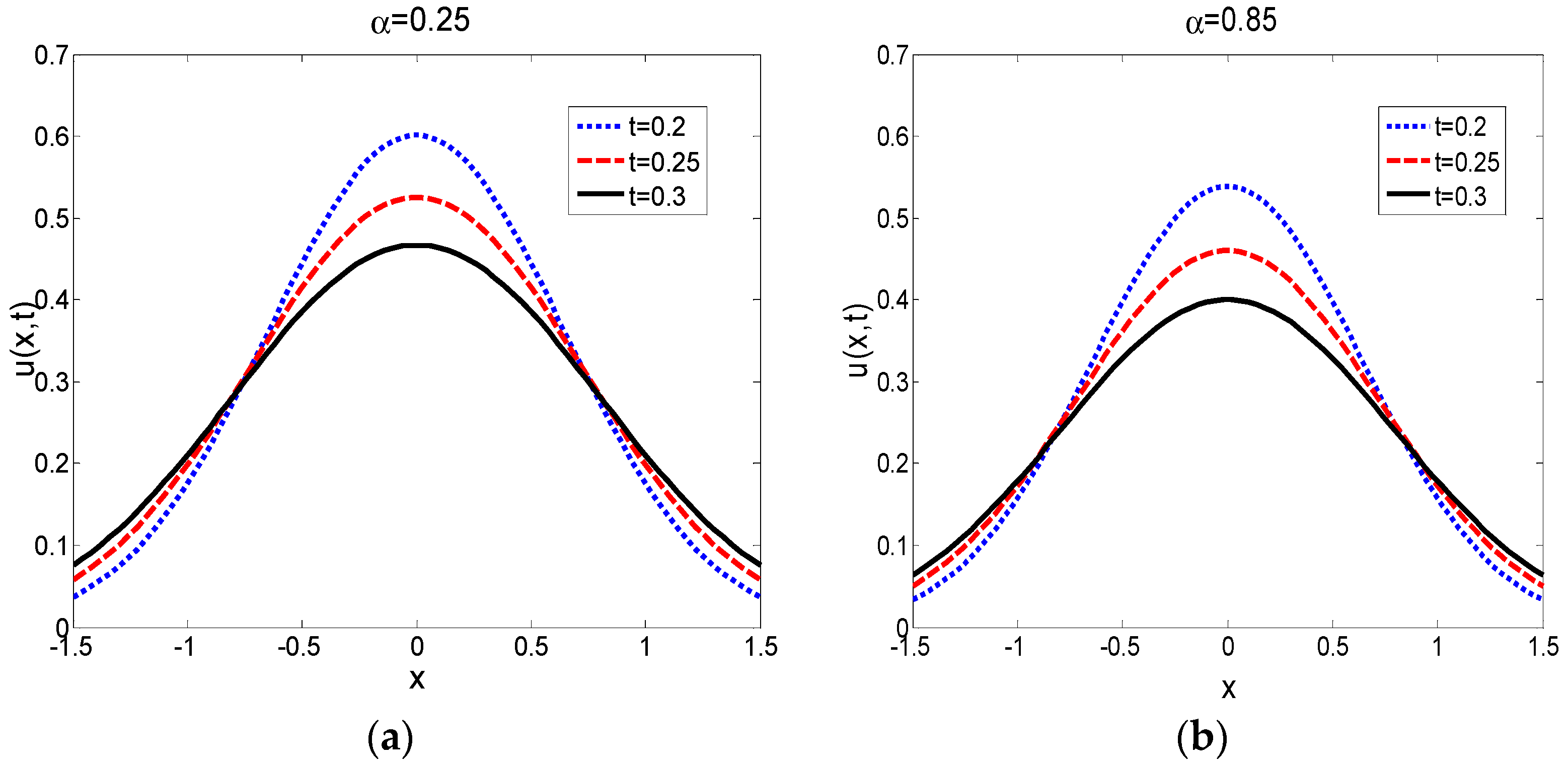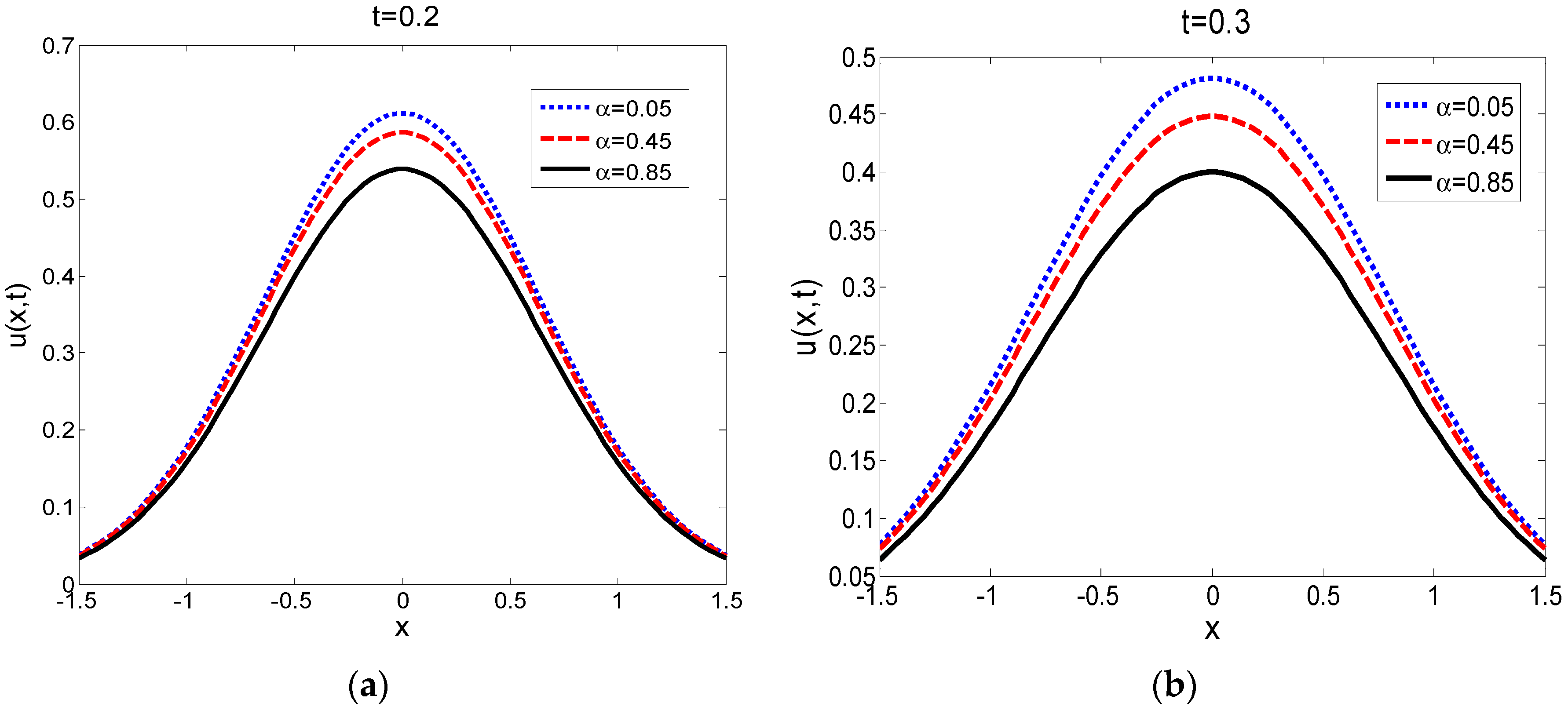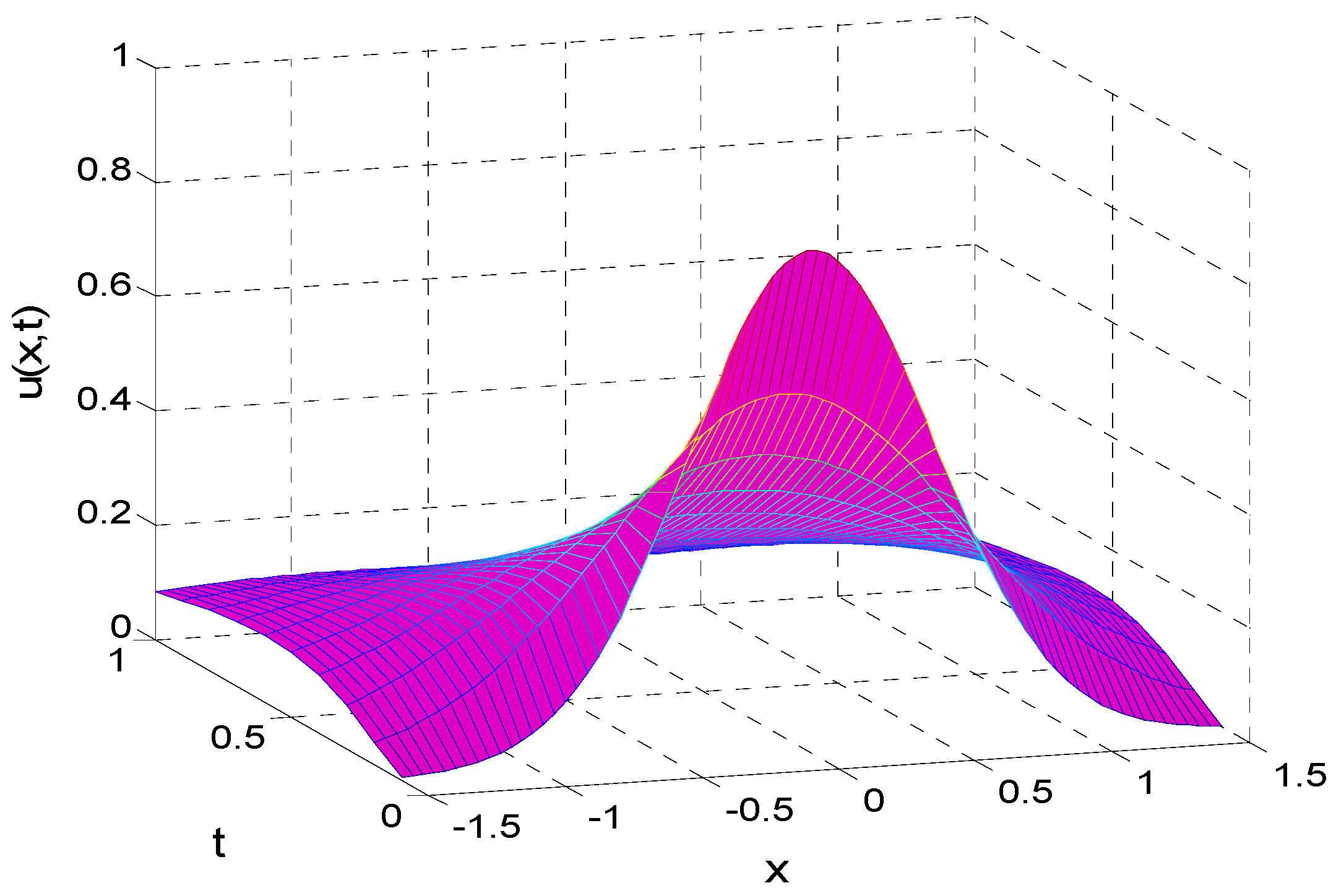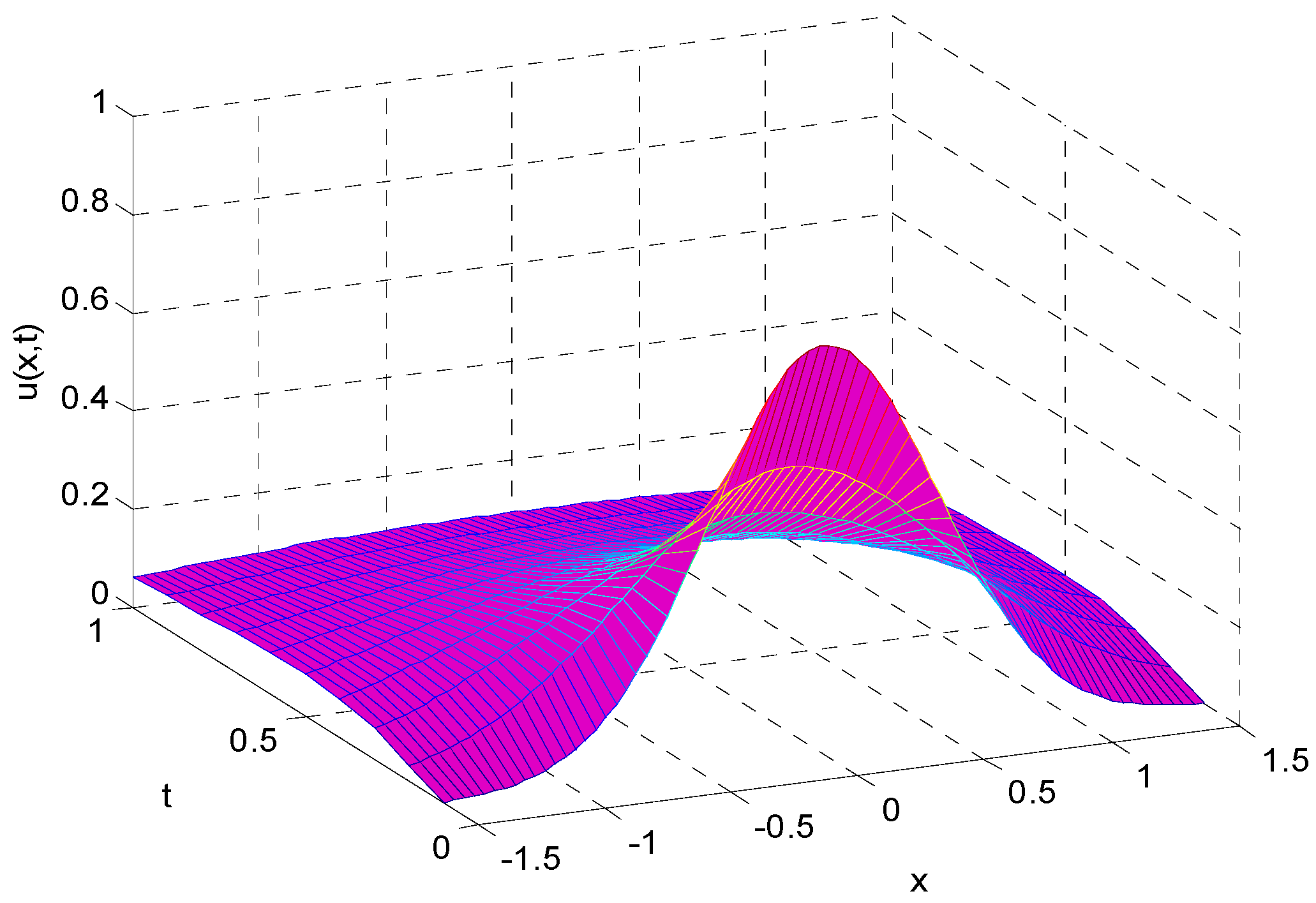It is worth mentioning that the analytical solution provided in Equation (24) can also be obtained by applying the references method [23,24,25] to Equation (23). In the end, some curves of the analytical solution are given, and the curves exhibit a long tail behavior for a large time. We found that a parabolic Volterra integro-differential equation with a power-law memory kernel is characterized by anomalous diffusion. The analytic solution of (1) can be found in some special cases, but in general it is difficult to obtain because of the non-local property of the integral term. Thus, in many cases, the more reasonable option is to find its numerical solution. Meanwhile, the analytical solutions we obtained from parabolic Volterra integro-differential equations with different types of frictional memory kernel provide great convenience for practical applications.

References

1. Han, H.; Zhu, L.; Brunner, H.; Brunner, H.; Ma, J. The numerical solution of parabolic Volterra integro-differential equations on unbounded spatial domains. Appl. Numer. Math. 2005, 55, 83–99. [Google Scholar] [CrossRef]
2. Lenzi, E.K.; Ribeiro, H.V.; Martins, J. Non-Markovian diffusion equation and diffusion in a porous catalyst. Chem. Eng. J. 2011, 172, 1083–1087. [Google Scholar] [CrossRef]
3. Lenzi, E.K.; Lenzi, M.K.; Rossato, R. Results for a fractional diffusion equation with a non-local term in spherical symmetry. Phys. Lett. A 2008, 372, 6121–6124. [Google Scholar] [CrossRef]
4. Habetler, G.J.; Schiffman, R.L. A finite difference method for analyzing the compression of poro-viscoelastic media. Computing 1970, 6, 342–348. [Google Scholar] [CrossRef]
5. Yanik, E.G.; Fairweather, G. Finite element methods for parabolic and hyperbolic partial integro-differential equations. Nonlinear Anal. Theory Methods Appl. 1988, 12, 785–809. [Google Scholar] [CrossRef]
6. Souplet, P. Blow-up in nonlocal reaction-diffusion equations. SIAM J. Math. Anal. 1998, 29, 1301–1334. [Google Scholar] [CrossRef]
7. Dehghan, M.; Shokri, A. A numerical method for two-dimensional Schrödinger equation using collocation and radial basis functions. Comput. Math. Appl. 2007, 54, 136–146. [Google Scholar] [CrossRef]
8. Dehghan, M.; Shakeri, F. Solution of parabolic integro-differential equations arising in heat conduction in materials with memory via He’s variational iteration technique. Int. J. Numer. Methods Biomed. Eng. 2010, 26, 705–715. [Google Scholar] [CrossRef]
9. Avazzadeh, Z.; Rizi, Z.B.; Ghaini, F.M.M. A numerical solution of nonlinear parabolic-type Volterra partial integro-differential equations using radial basis functions. Eng. Anal. Bound. Elem. 2012, 36, 881–893. [Google Scholar] [CrossRef]
10. Aguilar, M.; Brunner, H. Collocation methods for second-order Volterra integro-differential equations. Appl. Numer. Math. 1988, 4, 455–470. [Google Scholar] [CrossRef]
11. Fakhar-Izadi, F.; Dehghan, M. The spectral methods for parabolic Volterra integro-differential equations. Comput. Appl. Math. 2011, 235, 4032–4046. [Google Scholar] [CrossRef]
12. Murthy, A.S.V.; Verwer, J.G. Solving parabolic integro-differential equations by an explicit integration method. Comput. Appl. Math. 1992, 39, 121–132. [Google Scholar] [CrossRef]
13. Sandev, T.; Metzler, R.; Tomovski, Ž. Fractional diffusion equation with a generalized Riemann-Liouville time fractional derivative. J. Phys. A Math. Theor. 2011, 44, 255203. [Google Scholar] [CrossRef]
14. Prabhakar, T.R. A singular integral equation with a generalized Mittag Leffler function in the kernel. Yokohama Math. J. 1971, 19, 7–15. [Google Scholar]
15. Mathai, A.M.; Saxena, R.K.; Haubold, H.J. The H-Function: Theory and Applications; Springer: Berlin/Heidelberg, Germany, 2010. [Google Scholar]
16. Ding, X.L.; Jiang, Y.L. Analytical solutions for the multi-term time–space fractional advection-diffusion equations with mixed boundary conditions. Nonlinear Anal. RWA 2013, 14, 1026–1033. [Google Scholar] [CrossRef]
17. Srivastava, H.M.; Tomovski, Ž. Fractional calculus with an integral operator containing a generalized Mittag–Leffler function in the kernel. Appl. Math. Comput. 2009, 211, 198–210. [Google Scholar] [CrossRef]
18. Tomovski, Ž.; Sandev, T. Effects of a fractional friction with power-law memory kernel on string vibrations. Comput. Math. Appl. 2011, 62, 1554–1561. [Google Scholar] [CrossRef]
19. Tomovski, Ž.; Hilfer, R.; Srivastava, H.M. Fractional and operational calculus with generalized fractional derivative operators and Mittag-Leffler type functions. Integral Transform. Integral Transform. Spec. Funct. 2010, 21, 797–814. [Google Scholar] [CrossRef]
20. Li, C.; Deng, W.H.; Shen, X.Q. Exact solutions and their asymptotic behaviors for the averaged generalized fractional elastic models. Commun. Theor. Phys. 2014, 62, 443–450. [Google Scholar] [CrossRef]
21. Guo, G.; Chen, B.; Zhao, X. First passage time distribution of a modified fractional diffusion equation in the semi-infinite interval. Physica A 2015, 433, 279–290. [Google Scholar] [CrossRef]
22. Rangarajan, G.; Ding, M. Anomalous diffusion and the first passage time problem. Phys. Rev. E 2000, 62. [Google Scholar] [CrossRef]
23. Lv, L.J. Several Solution Methods and Applications of Fractional Singular Diffusion Equation. Ph.D. Thesis, Fu Dan University, Shanghai, China, 5 April 2012. [Google Scholar]
24. Langlands, T.A.M. Solution of a modified fractional diffusion equation. Physica A 2006, 367, 136–144. [Google Scholar] [CrossRef] [Green Version]
25. Qi, H.T.; Jiang, X.Y. Solutions of the space-time fractional Cattaneo diffusion equation. Physica A 2011, 390, 1876–1883. [Google Scholar] [CrossRef]
Figure 1. Graphical representation of the solution at different times with α = 0.25 , 0.85 . (a) The analytical solution u ( x , t ) in (52) for different times when parameter α is fixed, the peak of curves will decrease gradually with the increasing of the time. (b) The solution in (52) for different times when parameter α is fixed, the peak of curves distinct decrease gradually and lenitively with the increasing of time.
Entropy 18 00344 g001
Figure 2. Graphical representation of the solution with different parameters α at times t = 0.2 , 0.3. (a) Times is fixed, the peak of curves will decrease gradually with the increasing of parameter α . (b) The peak of curves distinct decrease and get fit with the increasing of parameter α under given time.
Entropy 18 00344 g002
Figure 3. Graphical representation of the solution with α = 0.25 .
Entropy 18 00344 g003
Figure 4. Graphical representation of the solution with α = 0.85 .
Entropy 18 00344 g004