Predicting Traffic Flow in Local Area Networks by the Largest Lyapunov Exponent

Abstract

The dynamics of network traffic are complex and nonlinear, and chaotic behaviors and their prediction, which play an important role in local area networks (LANs), are studied in detail, using the largest Lyapunov exponent. With the introduction of phase space reconstruction based on the time sequence, the high-dimensional traffic is projected onto the low dimension reconstructed phase space, and a reduced dynamic system is obtained from the dynamic system viewpoint. Then, a numerical method for computing the largest Lyapunov exponent of the low-dimensional dynamic system is presented. Further, the longest predictable time, which is related to chaotic behaviors in the system, is studied using the largest Lyapunov exponent, and the Wolf method is used to predict the evolution of the traffic in a local area network by both Dot and Interval predictions, and a reliable result is obtained by the presented method. As the conclusion, the results show that the largest Lyapunov exponent can be used to describe the sensitivity of the trajectory in the reconstructed phase space to the initial values. Moreover, Dot Prediction can effectively predict the flow burst. The numerical simulation also shows that the presented method is feasible and efficient for predicting the complex dynamic behaviors in LAN traffic, especially for congestion and attack in networks, which are the main two complex phenomena behaving as chaos in networks.

1. Introduction

From dynamic system viewpoint, a network is a complex nonlinear dissipative dynamic system in which there is a rich variety of nonlinear dynamic phenomena, such as traffic bursts, congestion, etc. [1,2]. Indeed, as a highly complex nonlinear system, the time sequence of network traffic, which includes a wide variety of chaotic attractors, is related to the complicated network traffic bursts, congestion, network attacks and so on [3,4]. Therefore, chaotic behaviors and their network traffic properties, have received increasingly more attention in recent years as a research new topic.

In practice, it is significant to study how to predict the changing of LAN traffic sampled at low resolution, that is, traffic prediction means to identify bursts or other singular phenomena in advance, and this will have an important significance for traffic control if the changing trend of the traffic has been predicted earlier and accurately. Moreover, it is also useful for designing congestion control, allocating resources and scheduling strategy efficiently, in order to mitigate or prevent congestion and make sufficient use of the network resources [5,6].

Traditionally, the prediction methods for the network traffic involve developing some empirical models such as fuzzy adaptive predictive method, autoregressive integrated moving average model, artificial neural networks method, and so on, instead of analyzing the real or sampled time sequences [7,8,9,10,11]. With the rapid development of nonlinear dynamics, it is shown that there exists a rich variety of nonlinear dynamics in the network traffic. To this end, a strategy, namely, the reconstruction of phase space based on the time sequence, is introduced in the prediction process, and by this method the local characteristics of flow rates can be captured directly from the real time sequence. In addition, it is well-known that there exists a butterfly-effect in chaotic systems, so the predictions of long-term behaviors maybe fail in the network traffic if the traditional model-based methods are used. Despite the issues mentioned above, the short-term behaviors can be predicted due to the slight divergence of the trajectories of the system in a sense.

Following the theories relevant to chaos, the phase space reconstruction based on time sequence, which the high-dimensional traffic can be projected onto, is introduced, and the relationships between the largest Lyapunov exponent and complicated network traffic are studied in this paper. Then, a numerical method is presented to compute the largest Lyapunov exponent, and the influences of parameters of the reconstructed phase space on the largest Lyapunov exponent are discussed further. Finally, as an example, the presented method is applied to predict LAN traffic.

2. Fundamental Theories

2.1. Phase Space Reconstructions for Time Sequences in Networks

As a complex nonlinear dissipative dynamic system, the long-term behaviors of LAN traffic will be attracted to a global compact, finite dimensional and invariant manifold. In practice, the invariant manifolds can be constructed by vast amounts of data, and then the original nonlinear dynamic system can be projected onto the invariant manifold and studied on it. It is clear that a low-dimensional dynamic model or mathematical model should be obtained directly from sampled high-dimensional data, before the largest Lyapunov exponent method is used to predict the change of the LAN traffic, that is, the phase space of the network traffic will be constructed. In 1980s, the famous Takens Theorem was proposed, and it is the basis of reconstructing the phase space of a system from which only the time sequence can be obtained [12]. For the sake of clarity, the process of phase space reconstruction for time sequences can be stated in brief as follows:

• Suppose there is a time sequence, x(t) = (x(t₁), x(t₂), …, x(t_n)), here x(t) is the sample, n the number of samples, t the time and Δt the sampling interval. The Euclidean subspace with m-dimensions can be constructed by the time sequence as a proper time lag τ = kΔt is chosen, and here k is a positive integer. The first point of the m-dimensional subspace includes m values, in which x(t₁) is the first element of the vector, x(t₁ + τ) is the next one, and the last one is x(t₁ + (m − 1)τ), so the first point in vector form in the phase space is defined as follows:

  $$Y_1=(x(t_1),x(t_1+\tau ),\cdots ,x(t_1+(m-1)\tau ))$$
• Then let x(t₂) be the first element in the vector, the second point in the m-dimensional subspace can be obtained further using the same method, that is:

  $$Y_2=(x(t_2),x(t_2+\tau ),\cdots ,x(t_2+(m-1)\tau ))$$
• The number of points in m-dimensional subspace is N = n − (m − 1)k, and all the points of the subspace are:

  $$\begin{array}{c}{Y}_1=(x(t_1),x(t_1+\tau ),\cdots ,x(t_1+(m-1)\tau ))\hfill \\ Y_2=(x(t_2),x(t_2+\tau ),\cdots ,x(t_2+(m-1)\tau ))\hfill \\ \cdots \cdots \hfill \\ Y_N=(x(t_n-(m-1)\tau ),x(t_n-(m-2)\tau ),\cdots ,x(t_n))\hfill \end{array}$$

  where Y_i can be considered as a point in the reconstructed phase space, including m elements.

So the network traffic can evolve in the m-dimensional phase space spanned by a set of vectors Y_i. Obviously, there are N points in m-dimensional phase space, and the lines connecting the phase points can describe the trajectory. In this study, C-C method is used to reconstruct the phase space.

2.2. C-C Method

In 1996, it was pointed out by Kugiumtzis [13] that the selection of the time lag τ should not be independent of the embedding dimension m, but be dependent on the time lag window τ_w, which is obtained by experiments and satisfies τ_w ≥ τ_p , where τ_p is the average trajectory period and can be obtained based on the spectra analysis of the time series [13]. Moreover, the relationship between τ_w and τ can be expressed by:

$${\tau }_w=\left(m-1\right)\tau$$

(1)

In 1999, the well-known C-C method is proposed by Kim and Eykholt [14]. The C-C method is a relatively simple method for computing the τ_w and τ by the correlation integral method, and then m could be obtained following Equation (1).

2.3. Physical Meaning of the Largest Lyapunov Exponent in Network

Lyapunov exponents λ can be used to analyze the spatial-temporal evolution of the system in the reconstructed phase space. Indeed, Lyapunov exponents are a measure for the sensitive dependence on initial conditions, and give the average growth factor of the relative distance between two adjacent trajectories in a unit time, which means this is a measure of the average divergent rate for adjacent trajectories. In summary, the physical meaning of λ in chaotic system can be expressed as follows [15]:

• As λ > 0, two trajectories diverge rapidly in phase space, and the long time behaviors of the dynamic system are sensitive to the initial conditions, implying the system is in a chaotic state.
• As λ = 0, two trajectories will not diverge or converge implying there is no chaos.
• As λ < 0, two trajectories in phase space converge, and the long time behaviors of dynamic system are not sensitive to the initial conditions, implying there is no chaos and the system is stable.

In the Lyapunov exponents, the largest Lyapunov exponent λ₁ can quantitatively describe the divergence rate of two adjacent trajectories in phase space, that is, it can measure the butterfly-effect, which is the chaotic behavior in time sequences. The butterfly-effect is a visual representation for randomness and uncertainness in dynamics, so λ₁ can be used as the quantitative index for the system. Due to the butterfly-effect of the chaotic system, it is difficult to predict the long-term behaviors by λ₁. However, λ₁ can be used to predict short-term behaviors. Moreover, the greater the value of λ₁ is, the shorter the time is needed for prediction due to the butterfly-effect [15,16].

2.4. Small Data Sets Method

There are some methods to compute largest Lyapunov exponent for time sequences, such as the Jacobian method, Wolf-algorithm, P-norm method, Small data sets method, etc. Among them, the common shortcoming of the Wolf-algorithm and Jacobian method are the poor computational results because of the non-uniform distribution of trajectories. The P-norm method can avoid the shortcoming of the above two methods by introducing parameter P, but it is difficult to choose the parameter P. However, the method of Small data sets method is reliable with small computation cost, and it is also easy to be carried out [17,18,19]. Hence, the Small data sets method will be used to compute the largest Lyapunov exponent λ₁ in this study. First, in the reconstructed phase space, the closest adjacent points on the certain trajectories at initial condition should be found. With a separating limit in short distance, it can be written as:

$$d_j(0)=\underset{k}{Min}\left|\right|Y_j-Y_k\left|\right|,\left|j-k\right|>P$$

(2)

where Y_k is one point in the neighbor of Y_j, and P is the average period of the time sequence.

After i steps, the distance between the closest adjacent points can be expressed as:

$$d_j(i)=\underset{k}{Min}\left|\right|Y_{j+i}-Y_{k+i}\left|\right|,i=1,2,...,\min (m-j,m-k)$$

(3)

where d_j(i) is the distance between the closest adjacent pair points j after i steps on the certain trajectories. Then, the largest Lyapunov exponent can be estimated by analyzing the average divergent rate of the closest adjacent points on the certain trajectories:

$${\lambda }_1(i)=\frac{1}{i\Delta t}\frac{1}{(N-i)}{\displaystyle \sum _{j=1}^{N-i}\ln \frac{d_j(i)}{d_j(0)}}$$

(4)

where $N=n-(m-1)k$, Δt is the sample period. To compute λ₁(i), for every i, the average value of all lnd_j(i) is calculated, that is:

$$y(i)=\frac{1}{q\Delta t}{\displaystyle \sum _{j=1}^q\ln d_j(i)}$$

(5)

where q is the number of d_j(i) which is not zero. The slope of the curve governed by Equation (5) is the largest Lyapunov exponent λ₁, and can be computed numerically by the least-squares approximate method [19].

2.5. Longest Predictable Duration

As an index, the largest Lyapunov exponent could describe the divergence of the initial trajectory at an exponential rate, and thus it can track the evolution trajectory of the dissipative systems in phase space. In particular, the divergence or convergence of the trajectories between neighbors in the time process means the unremembering or remembering the initial information, which relates to the predictability. Therefore, the largest Lyapunov exponent is a suitable parameter for predicting the chaotic system, and makes the prediction possible for the network traffic by studying the longest predictable time or duration.

Furthermore, chaotic motion is not random but deterministic, that is, the system is predictable within a certain critical period T₀. For a chaotic system, the largest Lyapunov exponent λ₁ describes the average divergent distance between Y_j+n and Y_k+n, which evolve after n iterations from the two adjacent phase points Y_j and Y_k, that is:

$$\frac{|Y_{j+n}-Y_{k+n}|}{d(0)}=e^{n{\lambda }_1}$$

(6)

$$d(0)=|Y_j-Y_k|$$

(7)

If $e^{n{\lambda }_1}$ exceeds a critical value C, it means that the trajectory are diverged too much to be predicted, and then the longest predictable time or duration is defined as the critical time T₀, that is:

$$C=\frac{|Y_{j+n}-Y_{k+n}|}{d(0)}=e^{T_0{\lambda }_1}$$

(8)

Then:

$$T_0=\frac{1}{{\lambda }_1}\ln C$$

(9)

Generally, set C = e, the longest predictable time or duration can be rewritten as:

$$T_0=\frac{1}{{\lambda }_1}$$

(10)

From the above equations, it is clear that the largest Lyapunov exponent can be used to predict the chaotic behaviors in the time sequence within a short-time [20].

2.6. Prediction Method Based on the Largest Lyaponov Exponent

In this study, the Wolf method is used to predict the traffic flow [18]. In the method, Y_j in phase space will be assumed as the predicted center point, and Y_k is the closest point with a distance d_j(0) from Y_j. Then, there exists a relation as follows:

$$d_j(0)=\left|\right|Y_j-Y_k\left|\right|$$

(11)

After evolvement with one step, Y_j and Y_k evolve into Y_j+1 and Y_k+1, respectively. Based on the physical meaning of the largest Lyapunov exponent mentioned above, the following equation can be obtained as:

$$\left|\right|Y_{j+1}-Y_{k+1}\left|\right|=\left|\right|Y_j-Y_k\left|\right|e^{{\lambda }_1}=d_j(0)e^{{\lambda }_1}$$

(12)

In Equation (12), x(t_n+1), the last component of the phase point Y_j+1, is the only unknown and could be obtained from the following equation:

$$Y_{j+1}(m)=Y_{k+1}(m)\pm \sqrt{{(d_j(0)e^{{\lambda }_1})}^2-{\displaystyle \sum _{i=1}^{m-1}{[Y_{j+1}(i)-Y_{k+1}(i)]}^2}}$$

(13)

Then, the predicted value $\widehat{x}(t_{n+1})$, which is used as known value in the following vector, can be obtained by:

$$\widehat{x}(t_{n+1})=Y_{j+1}(m)$$

(14)

3. Numerical Examples and Analysis

As an example, the largest Lyapunov exponent and its numerical method presented above are applied to the prediction of the traffic of a LAN. The real time sequence of LAN traffic used in this study is obtained from the internal network of a group of network monitoring systems, and the test time lasts from Monday to Sunday. Moreover, the LAN is an Ethernet host, the components of which are composed of hundreds of medium-sized local area networks, and the real time sequence is obtained by sniffing tools, namely, recording the number of network packets and the amount of data per second. The information used here includes web browsing, file transfer, network service systems, etc.

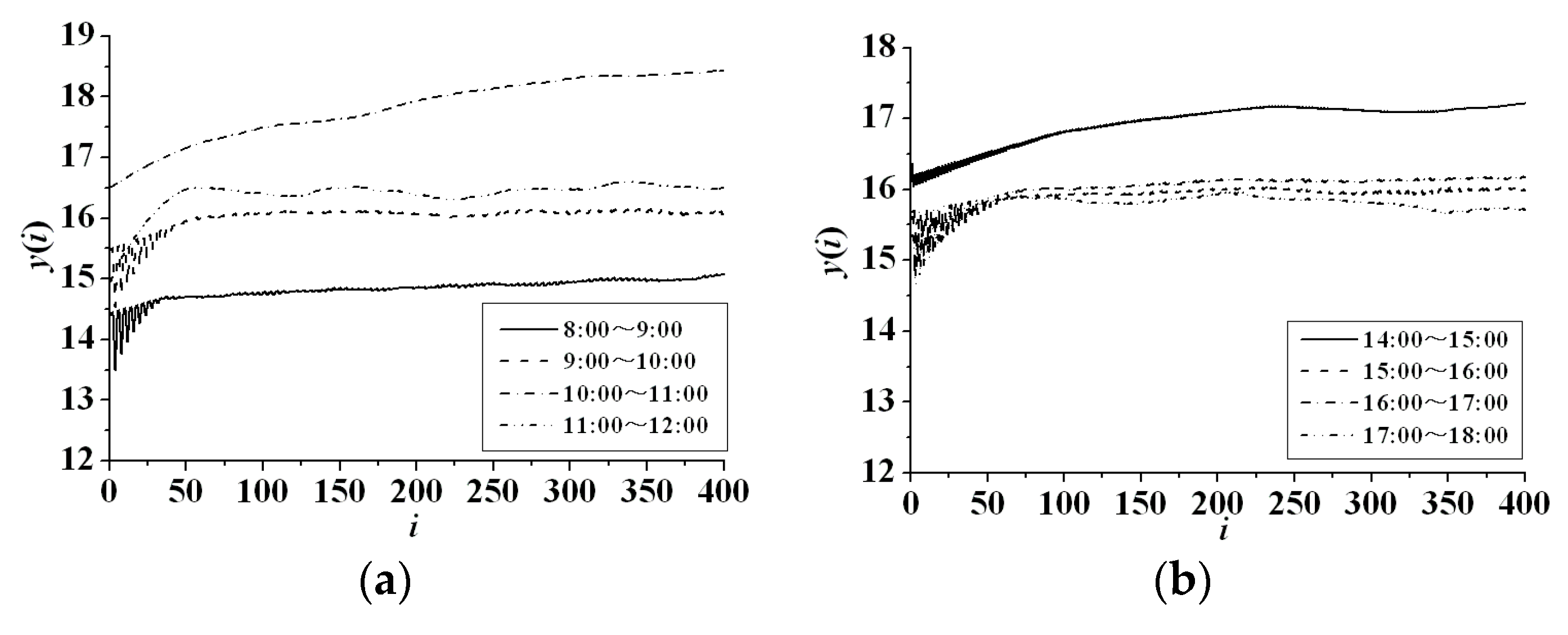
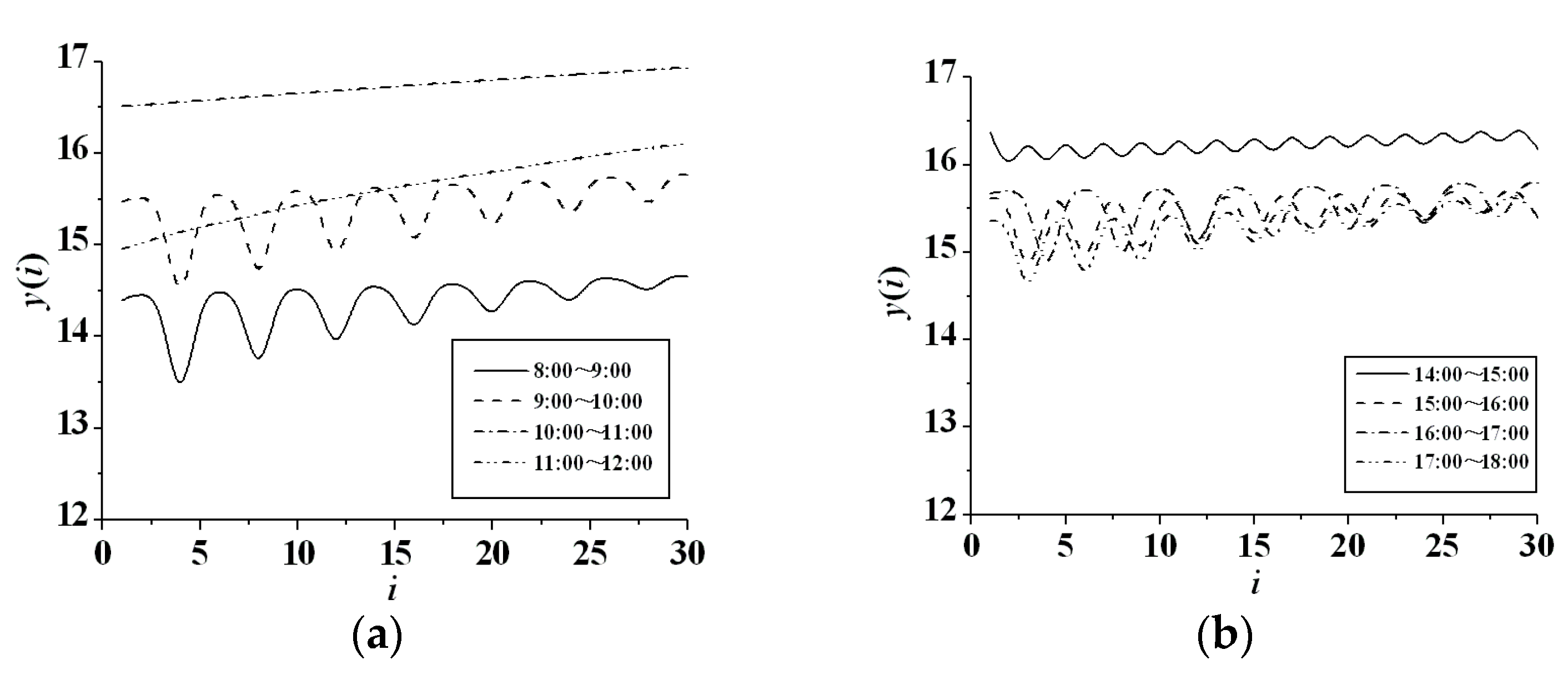
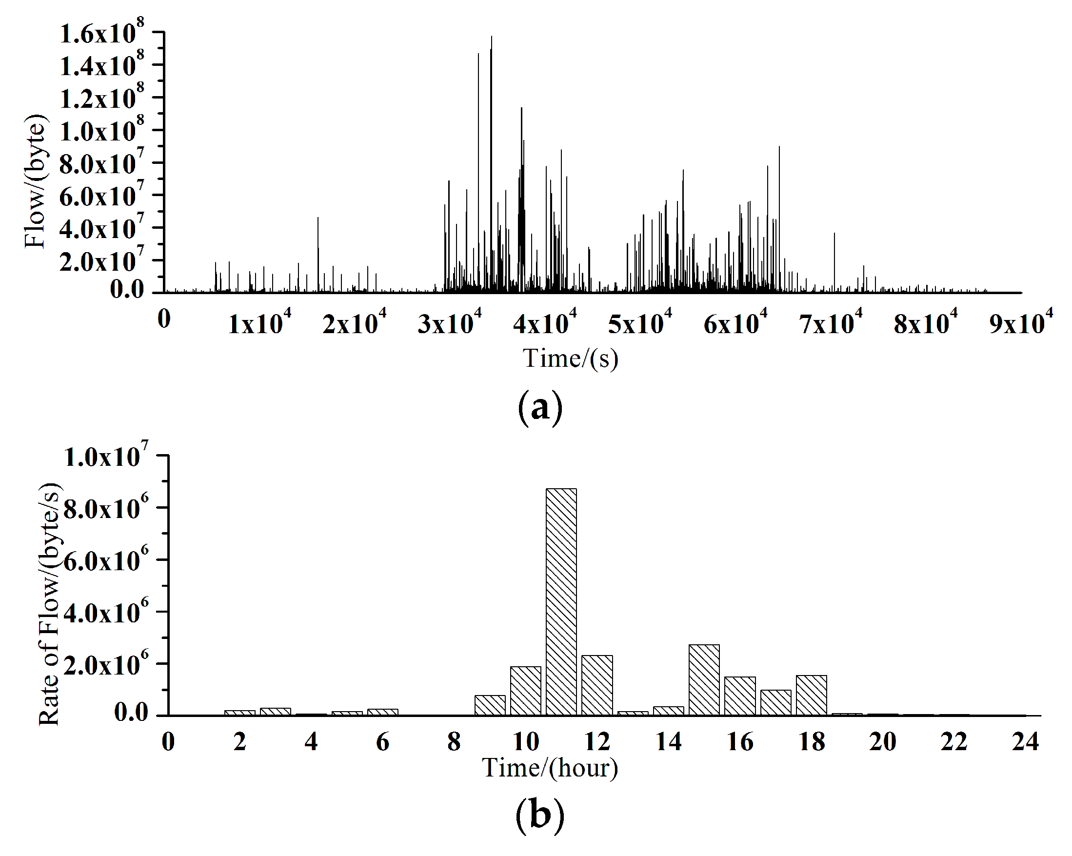
3.1. Largest Lyapunov Exponent of LAN Traffic

Figure 1 shows the real LAN traffic flow within one week, as well as the average daily traffic sequence, and the data are sampled from a business company. As shown in Figure 1, the usage of the network is lower on weekends than on working days, and the network usage is highest on Monday, implying the network can be easily congested in such period.

Figure 1. Real LAN traffic data in the week. (a) Real network traffic; (b) Average daily traffic sequence.

Therefore, the traffic sequence on Monday will be selected typically as an example to analyze in detail. Figure 2 is the real LAN traffic data and the average traffic flow per hour on Monday. Note that 8:00–12:00 and 14:00–18:00 are the working periods. It is clear that the usage of the network during rest periods is lower than that in working periods, so the chaotic characteristic of the working periods on Monday should be studied further.

Figure 2. Real LAN traffic data on Monday. (a) Real network traffic data; (b) Average traffic sequence per hour.

First, the C-C method is used to reconstruct the phase space. Following the above method, the average traffic sequence, time lag τ, embedding dimension m and average time lag window τ_w are computed numerically and shown in Table 1. The Small data sets method is used to compute the largest Lyapunov exponent of the network traffic sequence in the working periods. The changes of y(i) versus i in working period are shown in Figure 3, and Figure 4 shows the approximate linear part of Figure 3. The slope of the approximate linear part is computed by the least square method and its value is λ₁ shown in Table 1.

It is clear from Figure 4 that the slopes are greater than zero in this two periods, namely, 10:00–11:00 and 11:00–12:00, and the largest Lyapunov exponents are relatively greater, implying the system is obviously in a chaotic state.

Figure 3. y(i) in the working periods. (a) Morning; (b) Afternoon.

Figure 4. Approximate linear part of y(i) in the working periods. (a) Morning; (b) Afternoon.

Table 1. Parameters for network traffic in working periods.

Working Periods	8:00–9:00	9:00–10:00	10:00–11:00	11:00–12:00	14:00–15:00	15:00–16:00	16:00–17:00	17:00–18:00
Average traffic (byte/s)	772,602	1,881,664	8,721,630	2,313,709	2,731,960	1,504,641	985,395	1,555,366
τw	32	48	99	40	100	51	72	42
τ	4	4	1	1	2	3	4	3
m	9	13	100	41	51	18	19	15
λ1	0.0169	0.0171	0.0147	0.0386	0.0065	0.0103	0.0076	0.0178

Table 1. Parameters for network traffic in working periods.

Working Periods	8:00–9:00	9:00–10:00	10:00–11:00	11:00–12:00	14:00–15:00	15:00–16:00	16:00–17:00	17:00–18:00
Average traffic (byte/s)	772,602	1,881,664	8,721,630	2,313,709	2,731,960	1,504,641	985,395	1,555,366
τw	32	48	99	40	100	51	72	42
τ	4	4	1	1	2	3	4	3
m	9	13	100	41	51	18	19	15
λ1	0.0169	0.0171	0.0147	0.0386	0.0065	0.0103	0.0076	0.0178

However, for the other periods, the Lyapunov exponent fluctuates, that is, the slopes are changing from positive to negative, so the stochastic characteristics are greater than the chaotic characteristics in these periods. Moreover, as shown in Table 1, the largest Lyapunov exponent during 11:00–12:00 is the largest one among all the periods, implying that the divergence rate of two adjacent trajectories in the phase space is the most rapid one, the predictable time is the shortest, and the long-term prediction of the motion becomes weak, implying the butterfly-effect is strong in the period. Furthermore, it can be seen from Table 1 that there is no relationship between the largest Lyapunov exponent and network usage. The reason is that the largest Lyapunov exponent could describe the divergence rate of the phase space trajectory rather than the complexity of the network.

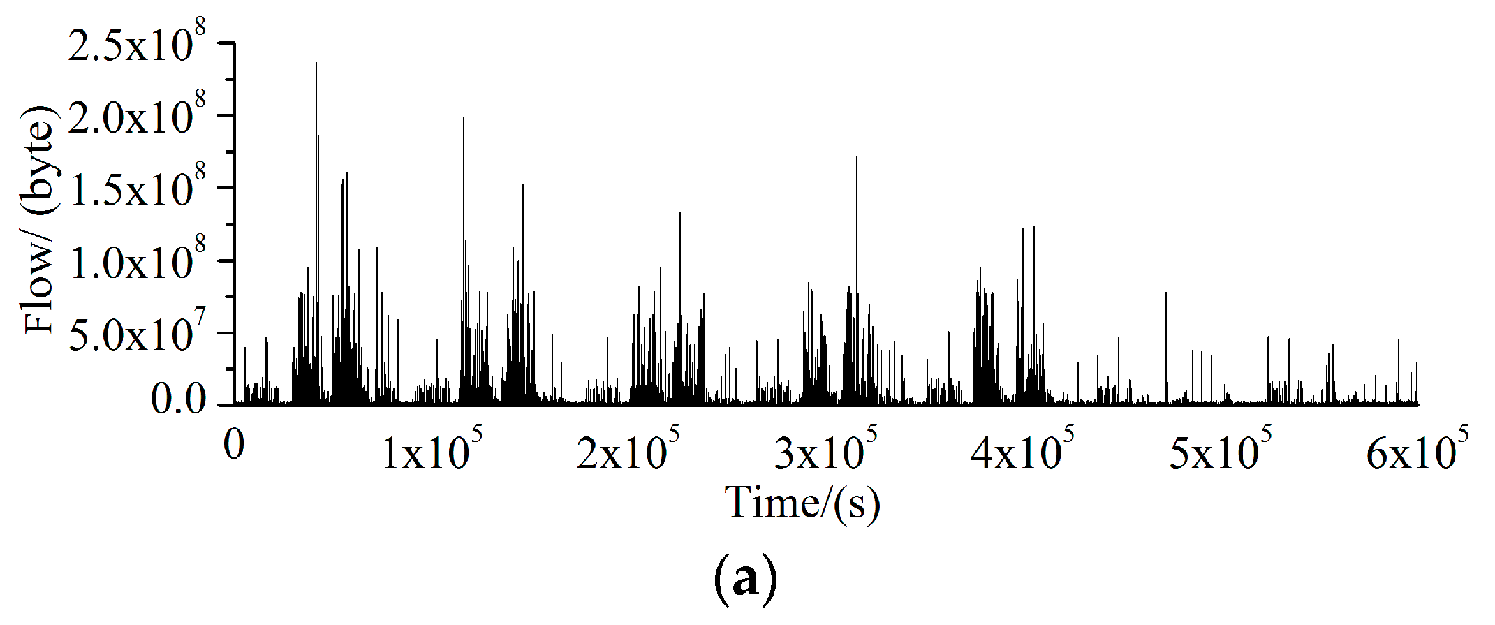
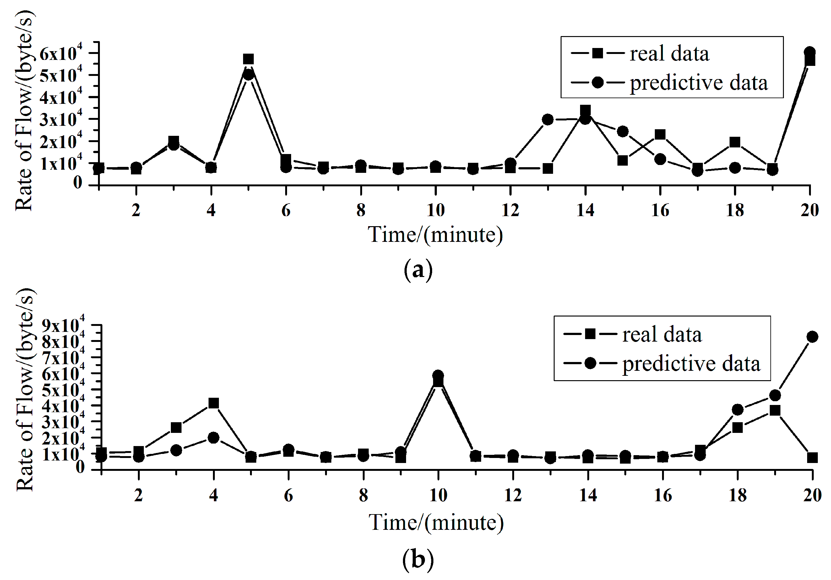
3.2. Prediction

In this section, the results are mainly obtained from dot prediction and interval prediction, which are the two typical methods. Dot prediction means that the average rate of flow will be predicted of the LAN. Interval prediction means the wide of the average rate of flow which the future traffic flow may fall into.

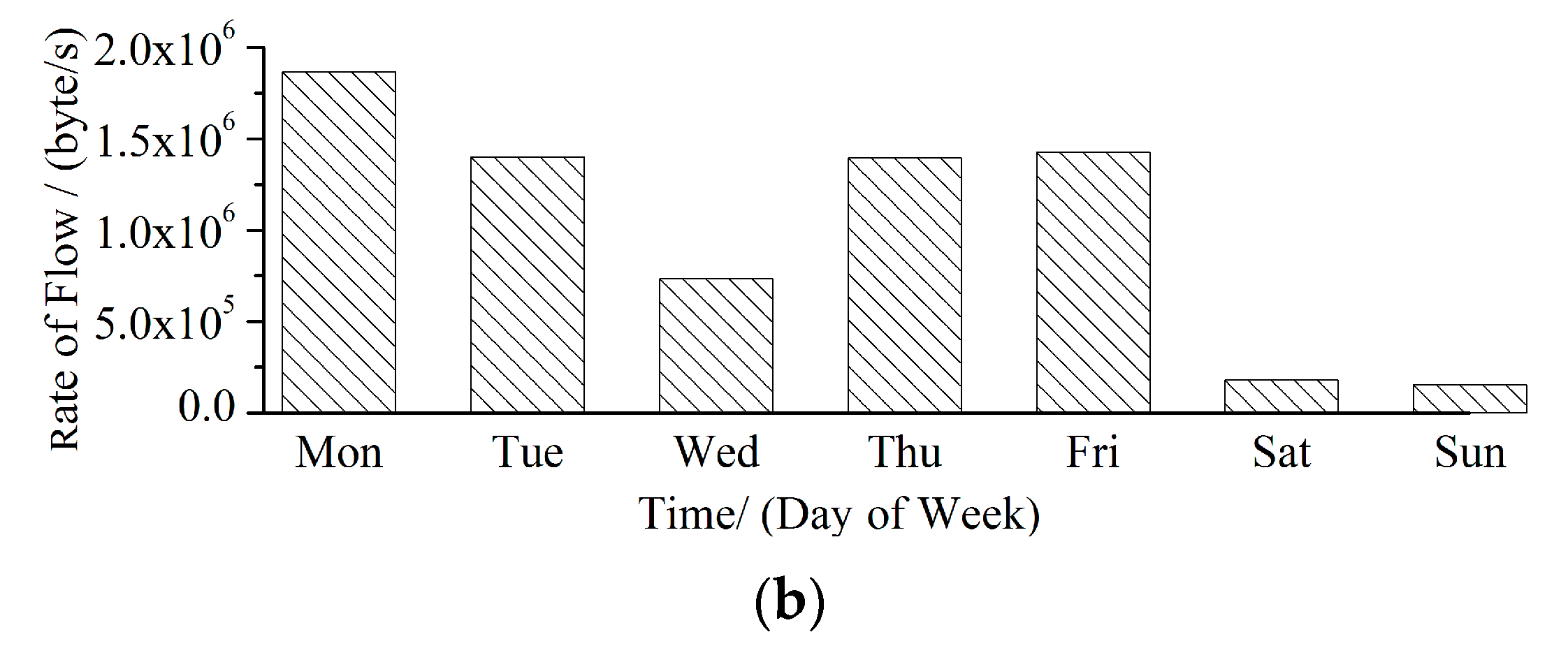
3.2.1. Dot Prediction

The LAN traffic data on Saturday and Sunday are chosen as an example of Dot Prediction, and the average rate of flow of the first 1400 min are considered. For convenience, the data from 1401 min to 1420 min in the traffic sequences are used in the analysis.

First, time lag τ and embedding dimension m are obtained by the C-C method. Then, the largest Lyapunov exponents are given by small data sets method, and the predictable time or duration are computed numerically. According to Equation (10), the maximum steps are six and seventeen for Saturday and Sunday, respectively, namely, 6 min and 17 min. In each process, the new predicted data is considered as the sample data regressing into the traffic sequence to predict the next one.

The real traffic sequence and the predicted traffic data for the two days are shown in Figure 5, and Table 2 lists the statistical results in the predictable time of the week. In Table 2, n obtained from Equation (10) means the maximum step of the data which could be predicted. Let f be the relative error, d₁ the real traffic data and d₂ the predicted traffic data. We have:

$$f=\left|\frac{d_1-d_2}{d_{1`}}\right|\times 100\%$$

(15)

Further, let n₁ be the number of the network traffic data as f is less than 10%, and n₂ the number of the network traffic data as f is less than 30%. Then, f₁ and f₂ are defined clearly as the probability density as follows:

$$f_1=(n_1/n)\times 100\%$$

(16)

$$f_2=(n_2/n)\times 100\%$$

(17)

It is clear that Dot Prediction can demonstrate the trend of fluctuation in the network traffic, especially in traffic congestion and burst states, which are the two main complex phenomena in the chaotic network. Moreover, as the duration is greater than the computed largest predictable time obtained by the largest Lyapunov exponent, the prediction precision becomes low. Moreover, the error becomes obvious after the traffic burst. In this case, it needs to undergo a period of adjustment to make the predicted data close to the real data again. To this end, the Interval Prediction is presented and used.

Figure 5. Predicted data and the real data of the network traffic. (a) Saturday; (b) Sunday.

Table 2. Results of network traffic in one week by Dot Prediction.

Date	Monday	Tuesday	Wednesday	Thursday	Friday	Saturday	Sunday
rate of flow (byte/s)	1.86538 × 106	1.40022 × 106	7.35079 × 105	1.39503 × 106	1.42701 × 106	1.80545 × 105	1.55155 × 105
τ	4	2	3	7	2	2	4
m	6	12	3	3	19	27	8
λ1	0.1848	0.0475	0.146	0.1562	0.044	0.1557	0.0606
n	5	21	7	6	23	6	17
f1(%)	60	71	57	67	52	83	41
f2(%)	80	90	86	100	91	100	71

Table 2. Results of network traffic in one week by Dot Prediction.

Date	Monday	Tuesday	Wednesday	Thursday	Friday	Saturday	Sunday
rate of flow (byte/s)	1.86538 × 106	1.40022 × 106	7.35079 × 105	1.39503 × 106	1.42701 × 106	1.80545 × 105	1.55155 × 105
τ	4	2	3	7	2	2	4
m	6	12	3	3	19	27	8
λ1	0.1848	0.0475	0.146	0.1562	0.044	0.1557	0.0606
n	5	21	7	6	23	6	17
f1(%)	60	71	57	67	52	83	41
f2(%)	80	90	86	100	91	100	71

3.2.2. Interval Prediction

Two results based on Equation (13) will be chosen as the prediction interval, namely, the reference or standard value, for network traffic sequence in one week, and the results are listed in Table 3, where n₃ is the number of the network traffic data which are included in the predicting interval. Then f₃ is defined as follows:

$$f_3=(n_3/n)\times 100\%$$

(18)

In order to avoid too large predict interval which would induces wrong result, Y_j+1(m) in Equation (13) should be limited to the neighbor of Y_k+1(m), the largest deviation value is selected in the 5% of Y_k+1(m) as follows:

$$Y_{j+1}(m)=Y_{k+1}(m)\pm 0.05\times Y_{k+1}(m)$$

(19)

After some computations and comparisons, it shows that the accuracy would become acceptable and can be improved for the sequential prediction if the small predicting value of the two results in Equation (13) is chosen as new historical data and added to the traffic sequences. The predicted results in Table 3 show that the most of real data are included in the predicting interval. Moreover, in comparison with the results shown in Table 2, the predicted results are more accurate in low average network traffic such as on the weekend. As the average traffic increases, the prediction accuracy becomes low. Hence, it can be concluded that the prediction method using the largest Lyapunov exponent, which is based on the divergence rate of two adjacent trajectories in phase space, is not available to the system with randomness, and the prediction possibility becomes weak for random signals, since the random components of the network traffic would increase with the average traffic increase.

Table 3. Results of interval prediction for network traffic sequences in one week.

Date	Monday	Tuesday	Wednesday	Thursday	Friday	Saturday	Sunday
n3	3	16	18	4	18	6	15
f3(%)	60	76	75	67	78	100	88

Table 3. Results of interval prediction for network traffic sequences in one week.

Date	Monday	Tuesday	Wednesday	Thursday	Friday	Saturday	Sunday
n3	3	16	18	4	18	6	15
f3(%)	60	76	75	67	78	100	88

4. Concluding Remarks

The results show that it is feasible to predict the flow rate of Local Area Network Traffic by the largest Lyapunov exponent. By the method presented, all the information from real traffic sequences can be used to reconstruct a phase space, so that the system can be studied in a low dimension reconstructed phase space, and a considerable amount of computation time can be saved. In particular, the feature of the method presented is that a low-dimensional dynamic model or mathematical model can be obtained directly from the sampled high-dimensional data via phase space reconstruction, and then the traffic characteristics extracted from the low-dimensional dynamic model would be used to predict the trend of the traffic.

References

- Liu, Y.; Zhang, J.; Mu, D. Nonlinear Dynamics of the Small-World Networks-Hopf Bifurcation, Sequence of Period-Doubling Bifurcations and Chaos. J. Phys. Conf. Ser. 2008, 96, 012061. [Google Scholar] [CrossRef]
- Chu, W.; Guan, X.; Cai, Z.; Gao, L. Real-Time Volume Control for Interactive Network Traffic. Comput. Netw. 2013, 57, 1611–1629. [Google Scholar] [CrossRef]
- Wang, J.; Yuan, J.; Li, Q.; Yuan, R. Correlation Dimension Based Nonlinear Analysis of Network Traffics with Different Application Protocols. Chin. Phys. B 2011, 20, 050506. [Google Scholar] [CrossRef]
- Feng, H.; Shu, Y.; Yang, O. Nonlinear Analysis of Wireless LAN Traffic. Nonlinear Anal. Real World Appl. 2009, 10, 1021–1028. [Google Scholar] [CrossRef]
- Nooruzzaman, M.; Koyama, O.; Katsuyama, Y. Congestion Removing Performance of Stackable ROADM in WDM Networks under Dynamic Traffic. Comput. Netw. 2013, 57, 2364–2373. [Google Scholar] [CrossRef]
- Sergiou, C.; Vassiliou, V.; Paphitis, A. Congestion Control in Wireless Sensor Networks through Dynamic Alternative Path Selection. Comput. Netw. 2014, 75, 226–238. [Google Scholar] [CrossRef]
- Chen, B.-S.; Yang, Y.-S.; Lee, B.-K.; Lee, T.-H. Fuzzy Adaptive Predictive Flow Control of ATM Network Traffic. IEEE Trans. Fuzzy Syst. 2003, 11, 568–581. [Google Scholar] [CrossRef]
- Alheraish, A. A Comparison of AR Full Motion Video Traffic Models in B-ISDN. Comput. Electr. Eng. 2005, 31, 1–22. [Google Scholar] [CrossRef]
- Szeto, W.Y.; Ghosh, B.; Basu, B.; O’Mahony, M. Multivariate Traffic Forecasting Technique Using Cell Transmission Model and SARIMA Model. J. Transp. Eng. ASCE 2009, 135, 658–667. [Google Scholar] [CrossRef]
- Zhang, N.; Zhang, Y.; Lu, H. Seasonal Autoregressive Integrated Moving Average and Support Vector Machine Models Prediction of Short-Term Traffic Flow on Freeways. Transp. Res. Rec. 2011, 2215, 85–92. [Google Scholar] [CrossRef]
- Swift, D.K.; Dagli, C.H. A Study on the Network Traffic of Connexion by Boeing: Modeling with Artificial Neural Networks. Eng. Appl. Artif. Intell. 2008, 21, 1113–1129. [Google Scholar] [CrossRef]
- Takens, F. Detecting Strange Attractors in Turbulence. Lect. Notes Math. 1981, 898, 361–381. [Google Scholar]
- Kugiumtzis, D. State Space Reconstruction Parameters in the Analysis of Chaotic Time Series. Physica D 1996, 95, 13–28. [Google Scholar] [CrossRef]
- Kim, H.S.; Eykholt, R.J.; Salas, D. Nonlinear Dynamics, Delay Times, and Embedding Windows. Physica D 1999, 127, 48–60. [Google Scholar] [CrossRef]
- David, R. Five Turbulent Problems. Physica D 1983, 7, 40–44. [Google Scholar]
- Boffetta, G.; Paladin, G.; Vulpiani, A. Strong Chaos without the Butterfly Effect in Dynamical Systems with Feedback. J. Phys. A Math. Gen. 1996, 29, 2291–2298. [Google Scholar] [CrossRef]
- Joach, M.H.; Erner, W.L. Lyapunov Exponents from Time Series of Acoustic Chaos. Phys. Rev. A 1989, 39, 2146–2152. [Google Scholar]
- Wolf, A.; Swift, J.B.; Swinney, H.L.; Vastano, J.A. Determining Lyapunov Exponent from a Time Series. Physica D 1985, 16, 285–317. [Google Scholar] [CrossRef]
- Rosenstein, M.T.; Collins, J.J.; Deluca, C.J. A Practical Method for Calculating Largest Lyapunov Exponents from Small Data Sets. Physica D 1993, 65, 117–134. [Google Scholar] [CrossRef]
- Luo, Y.; Wang, J.F.; Cao, C.X. A Prediction of Network Traffic Flow Based on Lyapunov Exponent. J. Chongqing Univ. 2004, 27, 28–30. [Google Scholar]
© 2016 by the authors; licensee MDPI, Basel, Switzerland. This article is an open access article distributed under the terms and conditions of the Creative Commons by Attribution (CC-BY) license (http://creativecommons.org/licenses/by/4.0/).
Share and Cite
Liu, Y.; Zhang, J. Predicting Traffic Flow in Local Area Networks by the Largest Lyapunov Exponent. Entropy 2016, 18, 32. https://doi.org/10.3390/e18010032
Liu Y, Zhang J. Predicting Traffic Flow in Local Area Networks by the Largest Lyapunov Exponent. Entropy. 2016; 18(1):32. https://doi.org/10.3390/e18010032
Chicago/Turabian StyleLiu, Yan, and Jiazhong Zhang. 2016. "Predicting Traffic Flow in Local Area Networks by the Largest Lyapunov Exponent" Entropy 18, no. 1: 32. https://doi.org/10.3390/e18010032
APA StyleLiu, Y., & Zhang, J. (2016). Predicting Traffic Flow in Local Area Networks by the Largest Lyapunov Exponent. Entropy, 18(1), 32. https://doi.org/10.3390/e18010032