Informational and Causal Architecture of Discrete-Time Renewal Processes

Abstract

Renewal processes are broadly used to model stochastic behavior consisting of isolated events separated by periods of quiescence, whose durations are specified by a given probability law. Here, we identify the minimal sufficient statistic for their prediction (the set of causal states), calculate the historical memory capacity required to store those states (statistical complexity), delineate what information is predictable (excess entropy), and decompose the entropy of a single measurement into that shared with the past, future, or both. The causal state equivalence relation defines a new subclass of renewal processes with a finite number of causal states despite having an unbounded interevent count distribution. We use the resulting formulae to analyze the output of the parametrized Simple Nonunifilar Source, generated by a simple two-state hidden Markov model, but with an infinite-state ϵ-machine presentation. All in all, the results lay the groundwork for analyzing more complex processes with infinite statistical complexity and infinite excess entropy.

1. Introduction

Stationary renewal processes are widely used, analytically tractable, compact models of an important class of point processes [1–4]. Realizations consist of sequences of events, e.g., neuronal spikes or earthquakes, separated by epochs of quiescence, the lengths of which are drawn independently from the same interevent distribution. Renewal processes on their own have a long history and, due to their offering a parsimonious mechanism, often are implicated in highly complex behavior [5–10]. Additionally, understanding more complicated processes [11–14] requires fully analyzing renewal processes and their generalizations.

As done here and elsewhere [15], analyzing them in-depth from a structural information viewpoint yields new statistical signatures of apparent high complexity: long-range statistical dependence, memory, and internal structure. To that end, we derive the causal-state minimal sufficient statistics, the ϵ-machine, for renewal processes and then derive new formulae for their various information measures in terms of the interevent count distribution. The result is a thorough-going analysis of their information architecture, a shorthand referring to a collection of measures that together quantify key process properties: predictability, difficulty of prediction, inherent randomness, memory, Markovity, and the like. The measures include:

• – the statistical complexity C_μ, which quantifies the historical memory that must be stored in order to predict a process’s future;

• – the entropy rate h_μ, which quantifies a process’ inherent randomness as the uncertainty in the next observation, even given that we can predict as well as possible;

• – the excess entropy E, which quantifies how much of a process’s future is predictable in terms of the mutual information between its past and future;

• – the bound information b_μ, which identifies the portion of the inherent randomness (h_μ) that affects a process’s future in terms of the information in the next observation shared with the future, above and beyond that of the entire past; and

• – the elusive information σ_μ, which quantifies a process’s deviation from Markovity as the mutual information between the past and future conditioned on the present.

Analyzing a process in this way gives a more detailed understanding of its structure and stochasticity. Beyond this, these information measures are key to finding limits to a process’s optimal lossy predictive features [16–19], designing action policies for intelligent autonomous agents [20], and quantifying whether or not a given process has one or another kind of infinite memory [21–23].

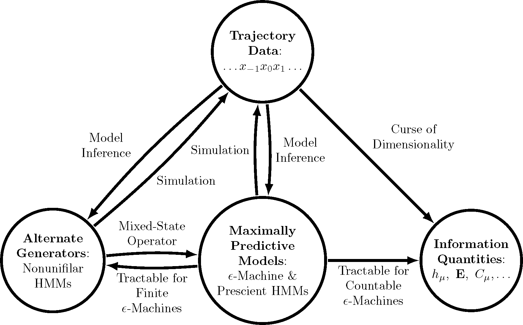
While it is certainly possible to numerically estimate information measures directly from trajectory data, statistical methods generally encounter a curse of dimensionality when a renewal process has long-range temporal correlations, since the number of typical trajectories grows exponentially (at entropy rate h_μ). Alternatively, we gain substantial advantages by first building a maximally-predictive model of a process (e.g., using Bayesian inference [24]) and then using that model to calculate information measures (e.g., using recently-available closed-form expressions when the model is finite [25]). Mathematicians have known for over a half century [26] that alternative models that are not maximally predictive are inadequate for such calculations. Thus, maximally-predictive models are critical. Figure 1 depicts the overall procedure just outlined, highlighting its important role. Here, extending the benefits of this procedure, we determine formulae for the information measures mentioned above and the appropriate structures for a class of processes that require countably infinite models: the ubiquitous renewal processes.

Our development requires familiarity with computational mechanics [27]. Those disinterested in its methods, but who wish to use the results, can skip to Figure 3a–d and

Table 1. Structural measures and information architecture of a stationary renewal process with interevent counts drawn from the distribution F(n), n ≥ 0, survival count distribution $w(n)={\displaystyle {\sum }_{m=n}^{\infty }F(m)}$, and mean interevent count $\mu ={\displaystyle {\sum }_{n=0}^{\infty }nF(n)<\infty }$. The function g(m, n) is defined by g(m, n) = F(m + n + 1) + F(m)F(n). Cases are needed for C_µ, but not other quantities, such as block entropy and information architecture quantities, since the latter can be calculated just as well from prescient machines. The quantities χ (crypticity) and $E(M,N)=I[X_{-M:0};X_{0:N}]$ are no less interesting than the others given here, but their expressions are not compact; see Appendix B.

Quantity	Expression
$C_{\mu }^{+}=H[{\mathcal{S}}^{+}]$	$-{\displaystyle {\sum }_{n=0}^{\infty }\frac{w(n)}{\mu +1}{\log }_2}\frac{w(n)}{\mu +1}\text{Not}\text{eventually}\mathrm{\Delta }\text{-Poisson}$ $-{\displaystyle {\sum }_{n=0}^{\tilde{n}-1}\frac{w(n)}{\mu +1}{\log }_2}\frac{w(n)}{\mu +1}{\displaystyle {\sum }_{m=0}^{\mathrm{\Delta }-1}\frac{{\displaystyle {\sum }_{k=0}^{\infty }w(\tilde{n}+k\mathrm{\Delta }+m)}}{\mu +1}{\log }_2\frac{{\displaystyle {\sum }_{k=0}^{\infty }w(\tilde{n}+k\mathrm{\Delta }+m)}}{\mu +1}}\text{eventually}\mathrm{\Delta }\text{-Poisson}$
E = I[X:0; X0:]	$-2{\displaystyle {\sum }_{n=0}^{\infty }\frac{w(n)}{\mu +1}{\log }_2}\frac{w(n)}{\mu +1}+{\displaystyle {\sum }_{n=0}^{\infty }(n+1)\frac{F(n)}{\mu +1}{\log }_2}\frac{F(n)}{\mu +1}$
hµ = H[X0|X:0]	$-\frac{1}{\mu +1}{\displaystyle {\sum }_{n=0}^{\infty }F(n){\log }_2}F(n)$
bµ = I[X1:; X0|X:0]	$\frac{1}{\mu +1}\left\{{\displaystyle {\sum }_{n=0}^{\infty }(n+1)F(n){\log }_2}F(n)-{\displaystyle {\sum }_{m,n=0}^{\infty }g(m,n){\log }_2}g(m,n)\right\}$
σµ = I[X1:; X:0|X0]	$\frac{1}{\mu +1}\left\{\mu {\log }_2\mu +{\displaystyle {\sum }_{n=0}^{\infty }nF(n){\log }_2}F(n)-2{\displaystyle {\sum }_{n=0}^{\infty }w(n){\log }_2}w(n)\right\}$
qµ = I[X1:; X0; X:0]	$\frac{1}{\mu +1}\left\{{\displaystyle {\sum }_{m,n=0}^{\infty }g(m,n){\log }_2}g(m,n)-{\displaystyle {\sum }_{n=0}^{\infty }w(n){\log }_{2}w(n)+(\mu +1){\log }_2}(\mu +1)-\mu {\log }_2\mu \right\}$
rµ = H[X0|X1:; X:0]	$\frac{1}{\mu +1}\left\{{\displaystyle {\sum }_{m,n=0}^{\infty }g(m,n)}{\log }_{2}g(m,n)-{\displaystyle {\sum }_{m,n=0}^{\infty }(n+2)F(n){\log }_{2}F(n)}\right\}$
H0 = H[X0]	$-\frac{1}{\mu +1}{\log }_2\frac{1}{\mu +1}-\left(1-\frac{1}{\mu +1}\right){\log }_2\left(1-\frac{1}{\mu +1}\right)$

. A pedagogical example is provided in Section 5. Two sequels will use the results to examine the limit of infinitesimal time resolution for information in neural spike trains [28] and the conditions under which renewal processes have infinite excess entropy [29].

The development is organized as follows. Section 2 provides a quick introduction to computational mechanics and prediction-related information measures of stationary time series. Section 3 identifies the causal states (in both forward and reverse time), the statistical complexity, and the ϵ-machine of discrete-time stationary renewal processes. Section 4 calculates the information architecture and predictable information of a discrete-time stationary renewal process in terms of the interevent count distribution. Section 5 calculates these information-theoretic measures for the parametrized simple nonunifilar source, a simple two-state hidden Markov model with a countable infinity of causal states. Finally, Section 6 summarizes the results and lessons, giving a view toward future directions and mathematical and empirical challenges.

2. Background

We first describe renewal processes, then introduce a small piece of information theory, review the definition of process structure, and, finally, recall several information-theoretic measures designed to capture organization in structured processes.

2.1. Renewal Processes

We are interested in a system’s immanent, possibly emergent, properties. To this end, we focus on behaviors and not, for example, particular equations of motion or particular forms of stochastic differential or difference equations. The latter are important in applications, because they are generators of behavior, as we will see shortly in Section 2.3. As Figure 1 explains, for a given process, some of its generators facilitate calculating key properties. Others lead to complicated calculations, and others still cannot be used at all.

As a result, our main object of study is a process $\mathcal{P}$: the list of all of a system’s behaviors or realizations {…, X₋₂, X₋₁, X₀, X₁, …} as specified by their measure μ (…, X₋₂, X₋₁, X₀, X₁, …). We denote a contiguous chain of random variables as X_0:l = X₀X₁ ⋯ X_L−1. Left indices are inclusive; right, exclusive. We suppress indices that are infinite. In this setting, the present X₀ is the random variable measured at t = 0; the past is the chain X_:0 = ⋯ X₋₂X₋₁ leading up the present; and the future is the chain following the present X_1: = X₁|X₂ ⋯. The joint probabilities Pr(X_0:N) of sequences are determined by the measure of the corresponding cylinder sets: Pr(X_0:N = x₀x₁ … x_N−1) = μ (…, x₀, x₁,…, x_n−1, …). Finally, we assume that a process is ergodic and stationary (Pr(X_0:L) = Pr(X_t:L+t) for all t, L ∈ Z) and that the observation values x_t range over a finite alphabet: $x\in \mathcal{A}$. In short, we work with hidden Markov processes [30].

Discrete-time stationary renewal processes here have binary observation alphabets A = {0, 1}. Observation of the binary symbol 1 is called an event. The event count is the number of 0’s between successive 1’s. Counts n are i.i.d. random variables drawn from an interevent distribution F(n), n ≥ 0. We restrict ourselves to persistent renewal processes, such that the probability distribution function is normalized: ${\displaystyle {\sum }_{n=0}^{\infty }F(n)=1}$. This translates into the processes being ergodic and stationary. We also define the survival function by $w(n)={\displaystyle {\sum }_{n^{\prime }=n}^{\infty }F(n^{\prime })}$, and the expected interevent count is given by $\mu ={\displaystyle {\sum }_{n=0}^{\infty }nF(n)}$. We assume also that μ < ∞.. It is straightforward to check that ${\displaystyle {\sum }_{n=0}^{\infty }w(n)=\mu +1}$.

Note the dual use of μ. On the one hand, it denotes the measure over sequences and, since it determines probabilities, it appears in names for informational quantities. On the other hand, it is commonplace in renewal process theory and denotes mean interevent counts. Fortunately, context easily distinguishes the meaning through the very different uses.

2.2. Process Unpredictability

The information or uncertainty in a process is often defined as the Shannon entropy H[X₀] of a single symbol X₀ [31]:

$$H[X_0]=-{\displaystyle \sum _{r\in \mathcal{A}}\mathrm{Pr}(X_0=x){\log }_2\mathrm{Pr}(X_0=x).}$$

(1)

However, since we are interested in general complex processes, those with arbitrary dependence structure, we employ the block entropy to monitor information in long sequences:

$$\begin{array}{l}H(L)=H[X_{0:L}]\\ =-{\displaystyle \sum _{w\in {\mathcal{A}}^L}\mathrm{Pr}(X_{0:L}=w){\log }_2\mathrm{Pr}}(X_{0:L}=w).\end{array}$$

To measure a process’s asymptotic per-symbol uncertainty, one then uses the Shannon entropy rate:

$$h_{\mu }=\underset{L\to \infty }{\lim }\frac{H(L)}{L}$$

when the limit exists. (Here and elsewhere, μ reminds us that information quantities depend on the process’s measure μ over sequences.) h_μ quantifies the rate at which a stochastic process generates information. Using standard informational identities, one sees that the entropy rate is also given by the conditional entropy:

$$h_{\mu }=\underset{L\to \infty }{\lim }H[X_0|X_{-L:0}]$$

(2)

This form makes transparent its interpretation as the residual uncertainty in a measurement given the infinite past. As such, it is often employed as a measure of a process’s degree of unpredictability.

2.3. Maximally Predictive Models

Forward-time causal states ${\mathcal{S}}^{+}$ are minimal sufficient statistics for predicting a process’s future [32,33]. This follows from their definition: a causal state ${\sigma }^{+}\in {\mathcal{S}}^{+}$ is a set of pasts grouped by the equivalence relation ~⁺:

$$x_{:0}{~}^{+}{x^{\prime }}_{:0}\iff \mathrm{Pr}(X_{0:}|X_{:0}=x_{:0})=\mathrm{Pr}(X_{0:}|X_{:0}={x^{\prime }}_{:0}).$$

(3)

Therefore, ${\mathcal{S}}^{+}$ is a set of classes, a coarse-graining of the uncountably infinite set of all pasts. At time t, we have the random variable ${\mathcal{S}}_t^{+}$ that takes values ${\sigma }^{+}\in {\mathcal{S}}^{+}$ and describes the causal-state process. $\dots ,{\mathcal{S}}_{-1}^{+},{\mathcal{S}}_0^{+},{\mathcal{S}}_1^{+},\dots .{\mathcal{S}}_t^{+}$ is a partition of pasts X_:t that, according to the indexing convention, does not include the present observation X_t. In addition to the set of pasts leading to it, a causal state ${\sigma }_t^{+}$ has an associated future morph: the conditional measure $\mathrm{\mu }(X_{t:}|{\sigma }_t^{+})$ of futures that can be generated from it. Moreover, each state ${\sigma }_t^{+}$ inherits a probability $\pi ({\sigma }_t^{+})$ from the process’s measure over pasts μ (X_:t). The forward-time statistical complexity is defined as the Shannon entropy of the probability distribution over forward-time causal states [32]:

$$C_{\mu }^{+}=H[{\mathcal{S}}_0^{+}].$$

(4)

A generative model is constructed out of the causal states by endowing the causal-state process with transitions:

$$T_{\sigma {\sigma }^{\prime }}^{(x)}=\mathrm{Pr}({\mathcal{S}}_{t+1}^{+}={\sigma }^{\prime },X_t=x|{\mathcal{S}}_t^{+}=\sigma ),$$

that give the probability of generating the next symbol x and ending in the next state σ′, if starting in state σ. (Residing in a state and generating a symbol do not occur simultaneously. Since symbols are generated during transitions there is, in effect, a half time step difference in the indexes of the random variables X_t and ${\mathcal{S}}_t^{+}$. We suppress notating this.) To summarize, a process’s forward-time ϵ-machine is the tuple $\{\mathcal{A},{\mathcal{S}}^{+},\{T^{(x)}:x\in \mathcal{A}\left\}\right\}$.

For a discrete-time, discrete-alphabet process, the ϵ-machine is its minimal unifilar hidden Markov model (HMM) [32,33]. (For a general background on HMMs, see [34–36].) Note that the causal state set can be finite, countable, or uncountable; the latter two cases can occur even for processes generated by finite-state HMMs. Minimality can be defined by either the smallest number of states or the smallest entropy over states [33]. Unifilarity is a constraint on the transition matrices T^(x), such that the next state σ′ is determined by knowing the current state σ and the next symbol x. That is, if the transition exists, then $\mathrm{Pr}({\mathcal{S}}_{t+1}^{+}|X_t=x,{\mathcal{S}}_t^{+}=\sigma )$ has support on a single causal state.

While the ϵ-machine is a process’s minimal, maximally-predictive model, there can be alternative HMMs that are as predictive, but are not minimal. We refer to the maximally-predictive property by referring to the ϵ-machine and these alternatives as prescient. The state and transition structure of a prescient model allow one to immediately calculate the entropy rate h_µ, for example. More generally, any statistic that gives the same (optimal) level of predictability we call a prescient statistic.

A similar equivalence relation can be applied to find minimal sufficient statistics for retrodiction [37]. Futures are grouped together if they have equivalent conditional probability distributions over pasts:

$$x_{0:}{~}^{-}{x^{\prime }}_{0:}\iff \mathrm{Pr}(X_{:0}|X_{0:}=x_{0:})=\mathrm{Pr}(X_{:0}|X_{0:}={x^{\prime }}_{0:})$$

(5)

A cluster of futures, a reverse-time causal state, defined by ~⁻, is denoted ${\sigma }^{-}\in {\mathcal{S}}^{-}$. Again, each σ⁻ inherits a probability π(σ⁻) from the measure over futures μ.(X_0:). Additionally, the reverse-time statistical complexity is the Shannon entropy of the probability distribution over reverse-time causal states:

$$C_{\mu }^{-}=H[{\mathcal{S}}_0^{-}].$$

(6)

In general, the forward and reverse-time statistical complexities are not equal [37,38]. That is, different amounts of information must be stored from the past (future) to predict (retrodict). Their difference $\Xi =C_{\mu }^{+}-C_{\mu }^{-}$ is a process’s causal irreversibility, and it reflects this statistical asymmetry.

Since we work with stationary processes in the following, the time origin is arbitrary and, so, we drop the time index t when it is unnecessary.

2.4. Information Measures for Processes

Shannon’s various information quantities—entropy, conditional entropy, mutual information, and the like—when applied to time series are functions of the joint distributions Pr(X_0:L). Importantly, they define an algebra of information measures for a given set of random variables [39]. The work in [40] used this to show that the past and future partition the single-measurement entropy H(X₀) into several distinct measure-theoretic atoms. These include the ephemeral information:

$$r_{\mu }=H[X_0|X_{:0,}{X}_{1:}],$$

(7)

which measures the uncertainty of the present knowing the past and future; the bound information:

$$b_{\mu }=I[X_0;X_{1:};X_{0:}],$$

(8)

which is the mutual information shared between present and future conditioned on the past; and the enigmatic information:

$$q_{\mu }=I[X_0;X_{:0};X_{1:}],$$

(9)

which is the three-way mutual information between past, present and future. Multi-way mutual information is sometimes referred to as co-information [40,41] and, compared to Shannon entropies and two-way mutual information, can have counterintuitive properties, such as being negative.

For a stationary time series, the bound information is also the shared information between present and past conditioned on the future:

$$b_{\mu }=I[X_0;X_{:0}|X_{1:}].$$

(10)

One can also consider the amount of predictable information not captured by the present:

$${\sigma }_{\mu }=I[X_{:0};X_{1:}|X_0].$$

(11)

This is called the elusive information [42]. It measures the amount of past-future correlation not contained in the present. It is nonzero if the process necessarily has hidden states and is therefore quite sensitive to how the state space is observed or coarse grained.

The maximum amount of information in the future predictable from the past (or vice versa) is the excess entropy:

$$\mathbf{E}=I[X_{:0}:X_{0:}].$$

It is symmetric in time and a lower bound on the stored informations $C_{\mu }^{+}$ and $C_{\mu }^{-}$. It is directly given by the information atoms above:

$$\mathbf{E}=b_{\mu }+{\sigma }_{\mu }+q_{\mu }$$

(12)

The process’s Shannon entropy rate h_µ (recall the form of Equation (2)) can also be written as a sum of atoms:

$$\begin{array}{c}{h}_{\mu }=H[X_0|X_{:0}]\\ =r_{\mu }+b_{\mu }.\end{array}$$

Thus, a portion of the information (h_µ) a process spontaneously generates is thrown away (r_µ), and a portion is actively stored (b_µ). Putting these observations together gives the information architecture of a single measurement (Equation (1)):

$$H[X_0]=q_{\mu }+2b_{\mu }+r_{\mu }.$$

(13)

These identities can be used to determine r_μ, q_μ, and E from H[X₀], b_μ, and σ_μ, for example.

We have a particular interest in when C_μ and E are infinite and, so, will investigate finite-time variants of causal states and finite-time estimates of statistical complexity and E. For example, the latter is given by:

$$\mathbf{E}(M,N)=I[X_{-M:0};X_{0:N}].$$

(14)

If E is finite, then $\mathbf{E}={\lim }_{M,N\to \infty }\mathbf{E}(M,N).$ When E is infinite, then the way in which E(M, N) diverges is one measure of a process’ complexity [21,43,44]. Analogous, finite past-future (M, N)-parametrized equivalence relations lead to finite-time forward and reverse causal states and statistical complexities $C_{\mu }^{+}(M,N)$ and $C_{\mu }^{-}(M,N)$.

3. Causal Architecture of Renewal Processes

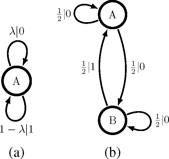
It will be helpful pedagogically to anchor our theory in the contrast between two different, but still simple, renewal processes. One is the familiar “memoryless” Poisson process with rate λ. Its HMM generator, a biased coin, is shown at the left of Figure 2. It has an interevent count distribution F(n) = (1 − λ)λⁿ; a distribution with unbounded support. However, we notice in Figure 2 that it is a unifilar model with a minimal number of states. Therefore, in fact, this one-state machine is the ϵ-machine of a Poisson process. The rate at which it generates information is given by the entropy rate: h_μ = H(λ) bits per output symbol. (Here, H(p) is the binary entropy function.) It also has a vanishing statistical complexity $C_{\mu }^{+}=0$ and, so, stores no historical information.

The second example is the Simple Nonunifilar Source (SNS) [45]; its HMM generator is shown in Figure 2b. Transitions from state B are unifilar, but transitions from state A are not. In fact, a little reflection shows that the time series produced by the SNS is a discrete-time renewal process. Once we observe the “event” x_t = 1, we know the internal model state to be σ_t+1 = A, so successive interevent counts are completely uncorrelated.

This SNS generator is not an ϵ-machine and, moreover, cannot be used to calculate the process’s information per output symbol (entropy rate). If we can only see 0’s and 1’s, we will usually be uncertain as to whether we are in state A or state B, so this generative model is not maximally predictive. How can we calculate this basic quantity? Additionally, if we cannot use the two-state generator, how many states are required, and what is their transition dynamic? The following uses computational mechanics to answer these and a number of related questions. To aid readability, though, we sequester most of the detailed calculations and proofs to Appendix A.

We start with a simple Lemma that follows directly from the definitions of a renewal process and the causal states. It allows us to introduce notation that simplifies the development.

Lemma 1. The count since last event is a prescient statistic of a discrete-time stationary renewal process.

That is, if we remember only the number of counts since the last event and nothing prior, we can predict the future as well as if we had memorized the entire past. Specifically, a prescient state $ℛ$ is a function of the past such that:

$$H[X_{0:}|X_{:0}]=H[X_{0:}|ℛ]$$

Causal states can be written as unions of prescient states [33]. We start with a definition that helps to characterize the converse; i.e., when the prescient states of Lemma 1 are also causal states.

To ground our intuition, recall that Poisson processes are “memoryless”. This may seem counterintuitive, if viewed from a parameter estimation point of view. After all, if observing longer pasts, one makes better and better estimates of the Poisson rate. However, finite data fluctuations in estimating model parameters are irrelevant to the present mathematical setting unless the parameters are themselves random variables, as in the nonergodic processes of [44]. This is not our setting here: the parameters are fixed. In fact, we restrict ourselves to studying ergodic processes, in which the conditional probability distributions of futures given pasts of a Poisson process are independent of the past.

We therefore expect the prescient states in Lemma 1 to fail to be causal states precisely when the interevent distribution is similar to that of a Poisson renewal process. This intuition is made precise by Definition 2.

Definition 1. A Δ-Poisson process has an interevent distribution:

$$F(n)=F(n\mathrm{mod}\mathrm{\Delta }){\lambda }^{[n/\mathrm{\Delta }]},$$

for all n and some λ > 0. If this statement holds for multiple Δ > 1, then we choose the smallest possible Δ.

Definition 2. A (ñ, Δ) eventually Δ-Poisson process has an interevent distribution that is Δ-Poisson for all n ≥ ñ:

$$F(\tilde{n}+k\mathrm{\Delta }+m)={\lambda }^{k}F(\tilde{n}+m),$$

for all 0 ≤ m < Δ, for all k ≥ 0, and for some λ > 0. If this statement holds for multiple Δ ≥ 1 and multiple ñ, then we choose the smallest possible Δ and the smallest possible ñ.

If this statement holds for multiple Δ ≥ 1 and multiple n, first, we choose the smallest possible Δ and, then, select the smallest possible n for that Δ. Order matters here.

Thus, a Poisson process is a Δ-Poisson process with Δ = 1 and an eventually Δ-Poisson process with Δ = 1 and ñ = 0. Moreover, we will now show that at some finite ñ, any renewal process is either: (i) Poisson, if Δ = 1; or (ii) a combination of several Poisson processes, if Δ > 1.

Why identify new classes of renewal process? In short, renewal processes that are similar to, but not the same as, the Poisson process do not have an infinite number of causal states. The particular condition for when they do not is given by the eventually Δ-Poisson definition. Notably, this new class is what emerged, rather unexpectedly, by applying the causal-state equivalence relation ~⁺ to renewal processes. The resulting insight is that general renewal processes, after some number of counts (the “eventually” part) and after some coarse-graining of counts (the Δ part), behave like a Poisson process.

With these definitions in hand, we can proceed to identify the causal architecture of discrete-time stationary renewal processes.

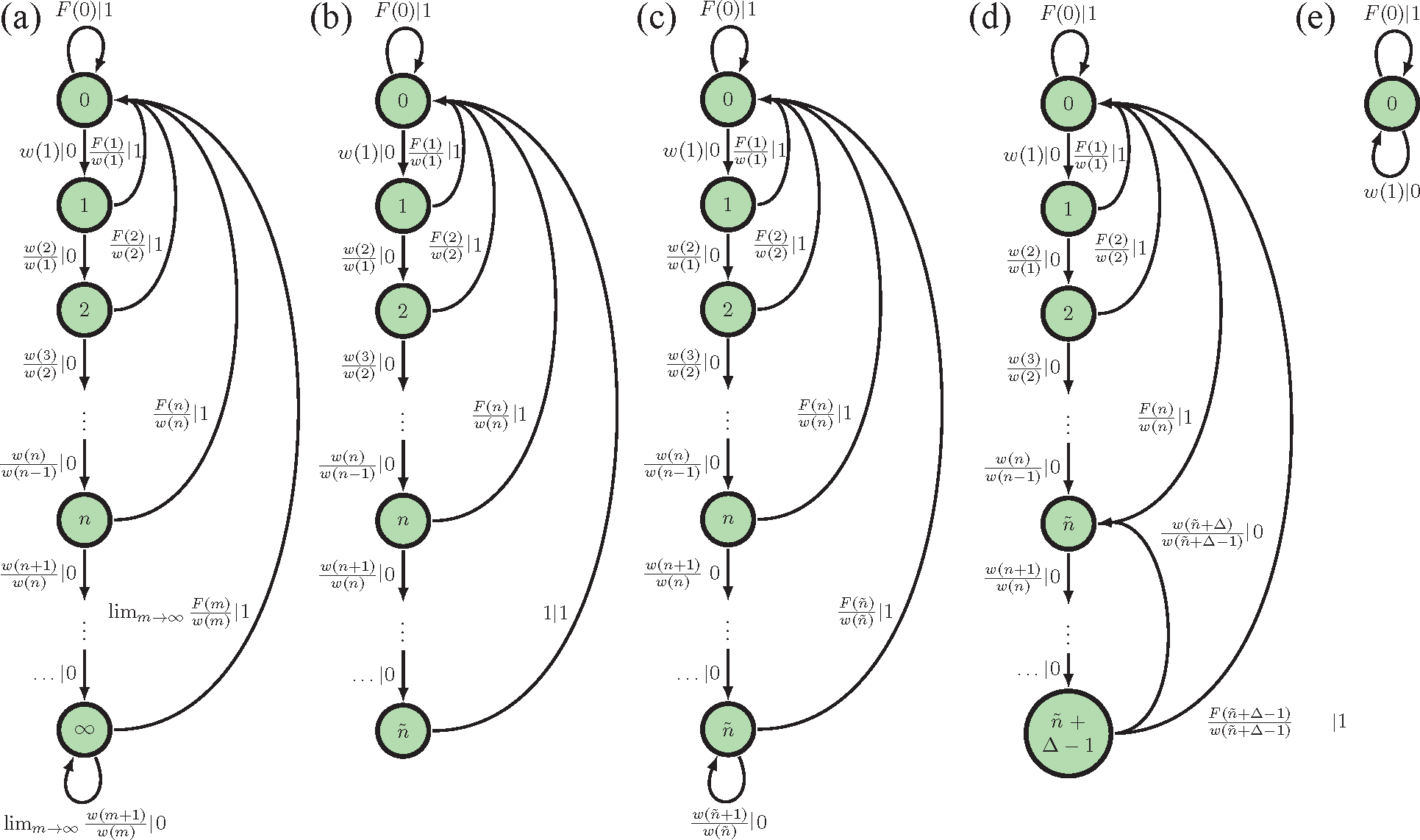
Theorem 1. (a) The forward-time causal states of a discrete-time stationary renewal process that is not eventually Δ-Poisson are groupings of pasts with the same count since the last event; (b) the forward-time causal states of a discrete-time eventually Δ-Poisson stationary renewal process are groupings of pasts with the same count since the last event up until n and pasts whose count n since the last event are in the same equivalence class as ñ modulo Δ.

The Poisson process, as an eventually Δ-Poisson with ñ = 0 and Δ = 1, is represented by the one-state ϵ-machine despite the unbounded support of its interevent count distribution. Unlike most processes, the Poisson process’ ϵ-machine is the same as its generative model shown in Figure 2a.

The SNS, on the other hand, has an interevent count distribution that is not eventually Δ-Poisson. According to Theorem 1, then, the SNS has a countable infinity of causal states despite its simple two-state generative model in Figure 2b. Compare Figure 3a. Each causal state corresponds to a different probability distribution over the internal states A and B. These internal state distributions are the mixed states of [46]. Observing more 0’s, one becomes increasingly convinced that the internal state is B. For maximal predictive power, however, we must track the probability that the process is still in state A. Both Figure 3a and Figure 2b are “minimally complex” models of the same process, but with different definitions of model complexity. We return to this point in Section 5.

Appendix A makes the statements in Theorem 1 precisely. The main result is that causal states are sensitive to two features: (i) eventually Δ-Poisson structure in the interevent distribution and (ii) the boundedness of F(n)’s support. If the support is bounded, then there are a finite number of causal states rather than a countable infinity of causal states. Similarly, if F(n) has Δ-Poisson tails, then there are a finite number of causal states despite the support of F(n) having no bound. Nonetheless, one can say that the generic discrete-time stationary renewal process has a countable infinity of causal states.

Finding the probability distribution over these causal states is straightforwardly related to the survival-time distribution w(n) and the mean interevent interval μ, since the probability of observing at least n counts since the last event is w(n). Hence, the probability of seeing n counts since the last event is simply the normalized survival function w(n)/(μ + 1). Appendix A derives the statistical complexity using this and Theorem 1. The resulting formulae are given in Table 1 for the various cases.

As described in Section 2, we can also endow the causal state space with a transition dynamic in order to construct the renewal process ϵ-machine: the process’s minimal unifilar hidden Markov model. The transition dynamic is sensitive to F(n)’s support and not only its boundedness. For instance, the probability of observing an event given that it has been n counts since the last event is F(n)/w(n). For the generic discrete-time renewal process, this is exactly the transition probability from causal state n to causal state 0. If F(n) = 0, then there is no probability of transition from σ = n to σ = 0. See Appendix A for details.

Figure 3a–d displays the causal state architectures, depicted as state-transition diagrams, for the ϵ-machines in the various cases delineated. Figure 3a is the ϵ-machine of a generic renewal process whose interevent interval can be arbitrarily large and whose interevent distribution never has exponential tails. Figure 3b is the ϵ-machine of a renewal process whose interevent distribution never has exponential tails, but cannot have arbitrarily large interevent counts. The ϵ-machine in Figure 3c looks quite similar to the ϵ-machine in Figure 3b, but it has an additional transition that connects the last state ñ to itself. This added transition changes our structural interpretation of the process. Interevent counts can be arbitrarily large for this ϵ-machine, but past an interevent count of ñ, the interevent distribution is exponential. Finally, the ϵ-machine in Figure 3d represents an eventually Δ-Poisson process with Δ > 1 whose structure is conceptually most similar to that of the ϵ-machine in Figure 3c. (See Definition 2 for the precise version of that statement.) If our renewal process disallows seeing interevent counts of a particular length L, then this will be apparent from the ϵ-machine, since there will be no transition between the causal state corresponding to an interevent count of L and causal state 0.

As described in Section 2, we can analytically characterize a process’ information architecture far better once we characterize its statistical structure in reverse time.

Lemma 2. Groupings of futures with the same counts to the next event are reverse-time prescient statistics for discrete-time stationary renewal processes.

Theorem 2. (a) The reverse-time causal states of a discrete-time stationary renewal process that is not eventually Δ-Poisson are groupings of futures with the same count to the next event; (b) the reverse-time causal states of a discrete-time eventually Δ-Poisson stationary renewal process are groupings of futures with the same count to the next event up until ñ plus groupings of futures whose count since the last event n are in the same equivalence class as ñ modulo Δ.

As a result, in reverse time, a stationary renewal process is effectively the same stationary renewal process: counts between events are still independently drawn from F(n). Thus, the causal irreversibility vanishes: Ξ = 0.

Moreover, these results taken together indicate that we can straightforwardly build a renewal process’s bidirectional machine from these forward and reverse-time causal states, as described in [37,38,46]. Additional properties can then be deduced from the bidirectional machine, but we leave this for the future.

In closing, we note a parallel in [47]: their A_t is the forward-time prescient statistic and E_t is the reverse-time prescient statistic. They call these the backward and forward recurrence times, respectively. They address continuous-time processes, however, and so, the setting differs somewhat.

4. Information Architecture of Renewal Processes

As Section 2 described, many quantities that capture a process’s predictability and randomness can be calculated from knowing the block entropy function H(L). Often, the block entropy is estimated by generating samples of a process and estimating the entropy of a trajectory distribution. This method has the obvious disadvantage that at large L, there are $|\mathcal{A}{|}^L$ possible trajectories and ${|\mathcal{A}|}^{h_{\mu }L}$ typical trajectories. Therefore, one easily runs into the problem of severe undersampling, previously referred to as the curse of dimensionality. This matters most when the underlying process has long-range temporal correlations.

Nor can one calculate the block entropy and other such information measures exactly from generative models that are not maximally predictive (prescient). Then, the model states do not shield the past from the future. For instance, as noted above, one cannot calculate the SNS’s entropy rate from its simple two-state generative HMM. The entropy of the next symbol given the generative model’s current state (A or B) actually underestimates the true entropy rate by assuming that we can almost always precisely determine the underlying model state from the past. For a sense of the fundamental challenge, see [26,48].

However, we can calculate the block entropy and various other information measures in closed-form from a maximally-predictive model. In other words, finding an ϵ-machine allows one to avoid the curse of dimensionality inherently involved in calculating the entropy rate, excess entropy, or the other information measures discussed here.

Figure 1 summarizes the above points. This section makes good on the procedure outlined there by providing analytic formulae for various information measures of renewal processes. The formulae for the entropy rate of a renewal process is already well known, but all others are new.

Prescient HMMs built from the prescient statistics of Lemma 1 are maximally predictive models and correspond to the unifilar hidden Markov model shown in Figure 3a. The prescient machines make no distinction between eventually Δ-Poisson renewal processes and ones that are not, but they do contain information about the support of F(n) through their transition dynamics (see Appendix A). Appendix B describes how a prescient machine can be used to calculate all information architecture quantities: r_μ, b_μ, σ_μ, q_μ, and the more familiar Shannon entropy rate h_μ and excess entropy E. A general strategy for calculating these quantities, as described in Section 2 and [19,40], is to calculate b_μ, h_μ, E and H[X₀] and then to derive the other quantities using the information-theoretic identities given in Section 2.

Table 1 gives the results of these calculations. It helps one’s interpretation to consider two base cases. For a Poisson process, we gain no predictive power by remembering specific pasts, and we would expect the statistical complexity, excess entropy, and bound information rate to vanish. The entropy rate and ephemeral information, though, are nonzero. One can check that this is, indeed, the case. For a periodic process with period T, in contrast, one can check that µ + 1 = T, since the period is the length of the string of 0’s (mean interevent interval µ) concatenated with the subsequent event x = 1. The statistical complexity and excess entropy of this process are log₂ T, and the entropy rate is h_μ = 0, as expected.

Calculating the predictable information E(M, N) requires identifying finite-time prescient statistics, since the predictable information is the mutual information between forward-time causal states over pasts of length M and reverse-time causal states over futures of length N. Such finite-time prescient statistics are identified in Corollary 1, below, and the predictable information is derived in Appendix B. The final expression is not included in Table 1 due to its length.

Corollary 1. Forward-time (and reverse-time) finite-time M prescient states of a discrete-time stationary renewal process are the counts from (and to) the next event up until and including M.

All of these quantities can be calculated using a mixed-state presentation, as described in [46], though the formulae developed there are as yet unable to describe processes with a countably infinite set of mixed states. Calculations of finite-time entropy rate estimates using a mixed-state presentation are consistent with all other results here, though. Purely for simplicity, we avoid discussing mixed-state presentations, though interested readers can find relevant definitions in [46].

5. Nonunifilar HMMs and Renewal Processes

The task of inferring an ϵ-machine for discrete-time, discrete-alphabet processes is essentially that of inferring minimal unifilar HMMs; what are sometimes also called “probabilistic deterministic” finite automata. In unifilar HMMs, the transition to the next hidden state given the previous one and next emitted symbol is determined. Nonunifilar HMMs are a more general class of time series models in which the transitions between underlying states given the next emitted symbol can be stochastic.

This simple difference in HMM structure has important consequences for calculating the predictable information, information architecture, and statistical complexity of time series generated by nonunifilar HMMs. First, note that for processes with a finite number of transient and recurrent causal states, these quantities can be calculated in closed form [25]. Second, the autocorrelation function and power spectrum can also be calculated in closed form for nonunifilar presentations [49]. Unlike these cases, though, most of Table 1’s quantities defy current calculational techniques. As a result, exact calculations of these prediction-related information measures for even the simplest nonunifilar HMMs can be surprisingly difficult.

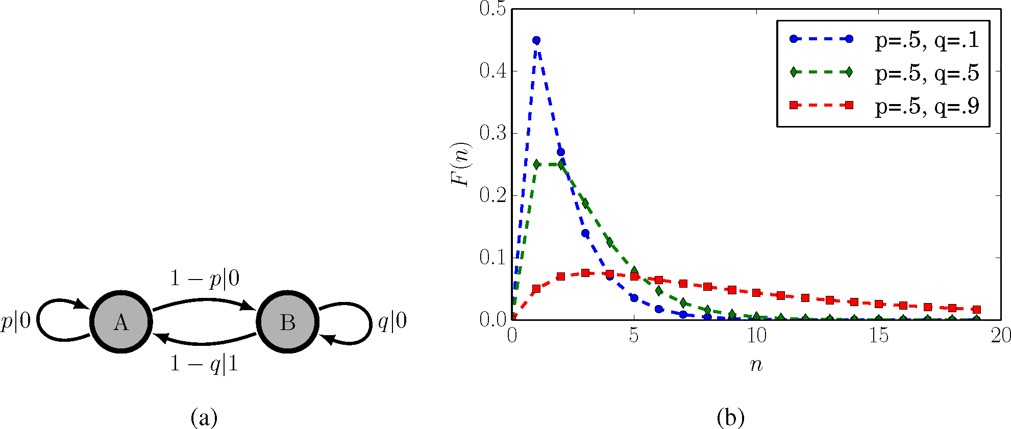
To illustrate this point, we focus our attention on a parametrized version of the SNS shown in Figure 4a. As for the original SNS in Figure 2, transitions from state B are unifilar, but transitions from state A are not. As noted before, the time series generated by the parametrized SNS is a discrete-time renewal process with interevent count distribution:

$$F(n)=\{\begin{array}{ll}(1-p)(1-q)(p^n-q^n)/(p-q)\hfill & p\ne q,\hfill \\ {(1-p)}^{2}n{p}^{n-1}\hfill & p=q.\hfill \end{array}$$

(15)

Figure 4b also shows F(n) at various parameter choices. The nonunifilar HMM there should be contrasted with the unifilar HMM presentation of the parametrized SNS, which is the ϵ-machine in Figure 3a, with a countable infinity of causal states.

Both parametrized SNS presentations are “minimally complex”, but according to different metrics. On the one hand, the nonunifilar presentation is a minimal generative model: No one-state HMM (i.e., biased coin) can produce a time series with the same statistics. On the other, the unifilar HMM is the minimal maximally-predictive model: In order to predict the future as well as possible given the entire past, we must at least remember how many 0’s have been seen since the last 1. That memory requires a countable infinity of prescient states. The preferred complexity metric is a matter of taste and desired implementation, modulo important concerns regarding overfitting or ease of inference [24]. However, if we wish to calculate the information measures in Table 1 as accurately as possible, finding a maximally predictive model, that is, a unifilar presentation, is necessary.

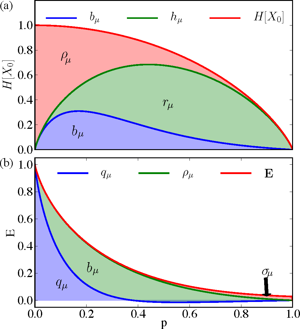
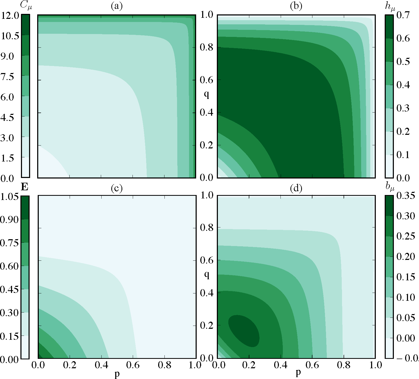
The SNS is not eventually A-Poisson with an unbounded-support interevent distribution. It can only be approximated by an eventually A-Poisson process. Therefore, one estimates its information anatomy via infinite sums. Using the formulae of Table 1, Figure 5 shows how the statistical complexity C_μ, excess entropy E, entropy rate h_µ, and bound information b_µ vary with the transition probabilities p and q. C_µ often reveals detailed information about a process’ underlying structure, but for the parametrized SNS and other renewal processes, the statistical complexity merely reflects the spread of the interevent distribution. Thus, it increases with increasing p and q. E, a measure of how much can be predicted rather than historical memory required for prediction, increases as p and q decrease. The intuition for this is that as p and q vanish, the process arrives at a perfectly predictable period-2 sequence. We see that the SNS constitutes a simple example of a class of processes over which information transmission between the past and future (E) and information storage (C_µ) are anticorrelated. The entropy rate h_µ in Figure 5b is maximized when transitions are uniformly stochastic and the bound information b_µ in Figure 5d is maximized somewhere between fully stochastic and fully deterministic regimes.

Figure 6 presents a more nuanced decomposition of the information measures as p = q vary from zero to one. Figure 6a breaks down the single-measurement entropy H[X₀] into redundant information ρ_μ in a single measurement, predictively useless generated information r_μ, and predictively useful generated entropy b_μ. As p increases, the SNS moves from mostly predictable (close to Period-2) to mostly unpredictable, shown by the relative height of the (green) line denoting h_μ to the (red) line denoting H[X₀]. The portion b_μ of h_μ predictive of the future is maximized at lower p when the single-measurement entropy is close to a less noisy Period-2 process. Figure 6b decomposes the predictable information E into the predictable information hidden from the present σ_μ, the predictable generated entropy in the present b_μ, and the co-information q_μ shared between past, present, and future. Recall that the co-information q_μ = E − σ_μ − b_μ can be negative, and for a large range of values, it is. Most of the predictable information passes through the present as indicated by σ_μ being small for most parameters p. Hence, even though the parametrized SNS is technically an infinite-order Markov process, it can be well approximated by a finite-order Markov process without much predictable information loss, as noted previously with rate distortion theory [50].

6. Conclusions

Stationary renewal processes are well studied, easy to define, and, in many ways, temporally simple. Given this simplicity and their long history, it is somewhat surprising that one is still able to discover new properties; in our case, by viewing them through an information-theoretic lens. Indeed, their simplicity becomes apparent in the informational and structural analyses. For instance, renewal processes are causally reversible with isomorphic ϵ-machines in forward and reverse-time, i.e., temporally reversible. Applying the causal-state equivalence relation to renewal processes, however, also revealed several unanticipated subtleties. For instance, we had to delineate new subclasses of renewal process (“eventually A-Poisson”) in order to completely classify ϵ-machines of renewal processes. Additionally, the informational architecture formulae in Table 1 are surprisingly complicated, since exactly calculating these informational measures requires a unifilar presentation. In Section 5, we needed an infinite-state machine to study the informational architecture of a process generated by simple two-state HMM.

Looking to the future, the new structural view of renewal processes will help improve inference methods for infinite-state processes, as it tells us what to expect in the ideal setting: what are the effective states, what are appropriate null models, how informational quantities scale, and the like. For example, Figure 3a–e gave all possible causal architectures for discrete-time stationary renewal processes. Such a classification will allow for more efficient Bayesian inference of ϵ-machines of point processes, as developed in [24]. That is, we can leverage “expert” knowledge that one is seeing a renewal process to delineate the appropriate subset of model architectures and thereby avoid searching over the superexponentially large set of all HMM topologies.

The range of the results’ application is much larger than that explicitly considered here. The formulae in Table 1 will be most useful for understanding renewal processes with infinite statistical complexity. For instance, [28] applies the formulae to study the divergence of the statistical complexity of continuous-time processes as the observation time scale decreases. Additionally, [29] applies these formulae to renewal processes with infinite excess entropy. In particular, there, we investigate the causal architectures of infinite-state processes that generate so-called critical phenomena: behavior with power-law temporal or spatial correlations [51]. The analysis of such critical systems often turns on having an appropriate order parameter. The statistical complexity and excess entropy are application-agnostic order parameters [52–54] that allow one to better quantify when a phase transition in stochastic processes has or has not occurred, as seen in [29]. Such critical behavior has even been implicated in early studies of human communication [55] (though, see [56,57]) and recently in neural dynamics [58] and in socially-constructed, communal knowledge systems [59].

References

- Smith, W.L. Renewal Theory and Its Ramifications. J. R. Stat. Soc. B 1958, 20, 243–302. [Google Scholar]
- Gerstner, W.; Kistler, W.M. Spiking Neuron Models: Single Neurons, Populations, Plasticity; Cambridge University Press: 2002; Chapter 5.2. [Google Scholar]
- Beichelt, F. Stochastic Processes in Science, Engineering and Finance; Chapman and Hall: New York, NY, USA, 2006. [Google Scholar]
- Barbu, V.S.; Limnios, N. Semi-Markov Chains and Hidden Semi-Markov Models toward Applications: Their Use in Reliability and DNA Analysis; Springer: Berlin/Heidelberg, Germany, 2008; Volume 191. [Google Scholar]
- Lowen, S.B.; Teich, M.C. Fractal Renewal Processes Generate 1/f Noise. Phys. Rev. E 1993, 47, 992–1001. [Google Scholar]
- Lowen, S.B.; Teich, M.C. Fractal Renewal Processes. IEEE Trans. Inf. Theory. 1993, 39, 1669–1671. [Google Scholar]
- Cakir, R.; Grigolini, P.; Krokhin, A.A. Dynamical Origin of Memory and Renewal. Phys. Rev. E 2006, 74, 021108. [Google Scholar]
- Akimoto, T.; Hasumi, T.; Aizawa, Y. Characterization of intermittency in renewal processes: Application to earthquakes. Phys. Rev. E 2010, 81, 031133. [Google Scholar]
- Montero, M.; Villarroel, J. Monotonic Continuous-time Random Walks with Drift and Stochastic Reset Events. Phys. Rev. E 2013, 87, 012116. [Google Scholar]
- Bologna, M.; West, B.J.; Grigolini, P. Renewal and Memory Origin of Anomalous Diffusion: A discussion of their joint action. Phys. Rev. E 2013, 88, 062106. [Google Scholar]
- Bianco, S.; Ignaccolo, M.; Rider, M.S.; Ross, M.J.; Winsor, P.; Grigolini, P. Brain Music Non-Poisson Renewal Processes. Phys. Rev. E 2007, 75, 061911. [Google Scholar]
- Li, C.B.; Yang, H.; Komatsuzaki, T. Multiscale Complex Network of Protein Conformational Fluctuations in Single-Molecule Time Series. Proc. Natl. Acad. Sci. USA 2008, 105, 536–541. [Google Scholar]
- Kelly, D.; Dillingham, M.; Hudson, A.; Wiesner, K. A New Method for Inferring Hidden Markov Models from Noisy Time Sequences. PLoS ONE 2012, 7, e29703. [Google Scholar]
- Onaga, T.; Shinomoto, S. Bursting Transition in a Linear Self-exciting Point Process. Phys. Rev. E 2014, 89, 042817. [Google Scholar]
- Valenza, G.; Citi, L.; Scilingo, E.P.; Barbieri, R. Inhomogeneous Point-Process Entropy: An Instantaneous measure of complexity in discrete systems. Phys. Rev. E 2014, 89, 052803. [Google Scholar]
- Shalizi, C.R.; Crutchfield, J.P. Information Bottlenecks, Causal States, and Statistical Relevance Bases: How to Represent Relevant Information in Memoryless Transduction. Adv. Complex Syst. 2002, 5, 91–95. [Google Scholar]
- Still, S.; Crutchfield, J.P. Structure or Noise? 2007, arXiv, 0708.0654.
- Still, S.; Crutchfield, J.P.; Ellison, C.J. Optimal Causal Inference: Estimating Stored Information and Approximating Causal Architecture. Chaos 2010, 20, 037111. [Google Scholar]
- Marzen, S.; Crutchfield, J.P. Information Anatomy of Stochastic Equilibria. Entropy 2014, 16, 4713–4748. [Google Scholar]
- Martius, G.; Der, R.; Ay, N. Information driven self-organization of complex robotics behaviors. PLoS ONE 2013, 8, e63400. [Google Scholar]
- Crutchfield, J.P.; Feldman, D.P. Regularities Unseen Randomness Observed: Levels of Entropy Convergence. Chaos 2003, 13, 25–54. [Google Scholar]
- Debowski, L. On Hidden Markov Processes with Infinite Excess Entropy. J. Theor. Prob. 2012, 27, 539–551. [Google Scholar]
- Travers, N.; Crutchfield, J.P. Infinite Excess Entropy Processes with Countable-State Generators. Entropy 2014, 16, 1396–1413. [Google Scholar]
- Strelioff, C.C.; Crutchfield, J.P. Bayesian Structural Inference for Hidden Processes. Phys. Rev. E 2014, 89, 042119. [Google Scholar]
- Crutchfield, J.P.; Riechers, P.; Ellison, C.J. Exact Complexity: Spectral Decomposition of Intrinsic Computation 2013, arXiv, 1309.3792, cond-mat.stat-mech.
- Blackwell, D. The Entropy of Functions of Finite-state Markov Chains; Transactions of the first Prague Conference on Information Theory, Statistical Decision Functions, Random Processes: Held at Liblice near Prague, from November 28 to 30, 1956, Publishing House of the Czechoslovak Academy of Sciences: Prague, Czech Republic, 1957; pp. 13–20. [Google Scholar]
- Crutchfield, J.P. Between Order Chaos. Nat. Phys. 2012, 8, 17–24. [Google Scholar]
- Marzen, S.E.; DeWeese, M.R.; Crutchfield, J.P. Time Resolution Dependence of Information Measures for Spiking Neurons: Atoms, Scaling and Universality 2015, arXiv, 1504.04756.
- Marzen, S.E.; Crutchfield, J.P. Long-Range Memory in Stationary Renewal Processes; 2015; in preparation. [Google Scholar]
- Ephraim, Y.; Merhav, N. Hidden Markov Processes. IEEE Trans. Inf. Theory. 2002, 48, 1518–1569. [Google Scholar]
- Cover, T.M.; Thomas, J.A. Elements of Information Theory, 2nd ed; Wiley: New York, NY, USA, 2006. [Google Scholar]
- Crutchfield, J.P.; Young, K. Inferring Statistical Complexity. Phys. Rev. Let 1989, 63, 105–108. [Google Scholar]
- Shalizi, C.R.; Crutchfield, J.P. Computational Mechanics: Pattern and Prediction, Structure and Simplicity. J. Stat. Phys. 2001, 104, 817–879. [Google Scholar]
- Paz, A. Introduction to Probabilistic Automata; Academic Press: New York, NY, USA, 1971. [Google Scholar]
- Rabiner, L.R.; Juang, B.H. An Introduction to Hidden Markov Models. IEEE ASSP Mag. 1986, 3, 4–16. [Google Scholar]
- Rabiner, L.R. A Tutorial on Hidden Markov Models and Selected Applications. IEEE Proc. 1989, 77, 257. [Google Scholar]
- Crutchfield, J.P.; Ellison, C.J.; Mahoney, J.R. Time’s Barbed Arrow: Irreversibility, Crypticity, and Stored Information. Phys. Rev. Lett. 2009, 103, 094101. [Google Scholar]
- Ellison, C.J.; Mahoney, J.R.; James, R.G.; Crutchfield, J.P.; Reichardt, J. Information Symmetries in Irreversible Processes. Chaos 2011, 21, 037107. [Google Scholar]
- Yeung, R.W. Information Theory and Network Coding; Springer: New York, NY, USA, 2008. [Google Scholar]
- James, R.G.; Ellison, C.J.; Crutchfield, J.P. Anatomy of a Bit: Information in a Time Series Observation. Chaos 2011, 21, 037109. [Google Scholar]
- Bell, A.J. The Co-information Lattice; Proceedings of the Fourth International Symposium on Independent Component Analysis and Blind Signal Separation, Nara, Japan, 1–4 April 2003, Amari, S.-i., Cichocki, A., Makino, S., Murata, N., Eds.; Springer: New York, NY, USA, 2003; pp. 921–926. [Google Scholar]
- Ara, P.M.; James, R.G.; Crutchfield, J.P. The Elusive Present: Hidden Past and Future Correlation and Why We Build Models 2015, arXiv, 1507.00672.
- Crutchfield, J.P.; Young, K. Computation at the Onset of Chaos. In Entropy, Complexity, and the Physics of Information; SFI Studies in the Sciences of Complexity; Zurek, W., Ed.; Addison-Wesley: Reading, MA, USA, 1990; Volume VIII, pp. 223–269. [Google Scholar]
- Bialek, W.; Nemenman, I.; Tishby, N. Predictability Complexity Learning. Neural Comp. 2001, 13, 2409–2463. [Google Scholar]
- Crutchfield, J.P. The Calculi of Emergence: Computation, Dynamics, and Induction. Physica D 1994, 75, 11–54. [Google Scholar]
- Ellison, C.J.; Mahoney, J.R.; Crutchfield, J.P. Prediction Retrodiction the Amount of Information Stored in the Present. J. Stat. Phys. 2009, 136, 1005–1034. [Google Scholar]
- Godreche, C.; Majumdar, S.N.; Schehr, G. Statistics of the Longest Interval in Renewal Processes. J. Stat. Mech. 2015, P03014. [Google Scholar] [CrossRef]
- Birch, J.J. Approximations for the Entropy for Functions of Markov Chains. Ann. Math. Stat. 1962, 33, 930–938. [Google Scholar]
- Riechers, P.M.; Varn, D.P.; Crutchfield, J.P. Pairwise Correlations in Layered Close-Packed Structures. Acta Cryst. A 2015, 71, 423–443. [Google Scholar]
- Still, S.; Ellison, C.J.; Crutchfield, J.P. Optimal Causal Inference: Estimating stored information and approximating causal architecture. Chaos 2010, 20, 037111. [Google Scholar]
- Crutchfield, J.P. Critical Computation Phase Transitions, and Hierarchical Learning. In Towards the Harnessing of Chaos; Yamaguti, M., Ed.; Elsevier Science: Amsterdam, The Netherlands, 1994; pp. 29–46. [Google Scholar]
- Crutchfield, J.P.; Feldman, D.P. Statistical Complexity of Simple One-Dimensional Spin Systems. Phys. Rev. E 1997, 55, R1239–R1243. [Google Scholar]
- Feldman, D.P.; Crutchfield, J.P. Structural Information in Two-Dimensional Patterns: Entropy Convergence and Excess Entropy. Phys. Rev. E 2003, 67, 051103. [Google Scholar]
- Tchernookov, M.; Nemenman, I. Predictive Information in a Nonequilibrium Critical Model. J. Stat. Phys. 2013, 153, 442–459. [Google Scholar]
- Zipf, G.K. The Psycho-Biology of Language: An Introduction to Dynamic Philology; Houghton Mifflin Company: Boston, MA, USA, 1935. [Google Scholar]
- Mandelbrot, B. An informational theory of the statistical structure of languages. In Communication Theory; Jackson, W., Ed.; Butterworths: London, UK, 1953; pp. 486–502. [Google Scholar]
- Miller, G.A. Some effects of intermittent silence. Am. J. Psychiatry 1957, 70, 311–314. [Google Scholar]
- Beggs, J.M.; Plenz, D. Neuronal Avalanches in Neocortical Circuits. J. Nuerosci. 2003, 23, 11167–11177. [Google Scholar]
- Dedeo, S. Collective Phenomena and Non-Finite State Computation in a Human Social System. PLoS ONE 2013, 8, e75808. [Google Scholar]
- Cessac, B.; Cofre, R. Spike Train statistics and Gibbs Distributions. J. Physiol. Paris. 2013, 107, 360–368. [Google Scholar]