
2D Anisotropic Wavelet Entropy with an Application to Earthquakes in Chile

1
Institute of Statistics, University of Valparaiso, Av. Gran Bretaña 1111 , Valparaiso, Chile
2
Institute of Mathematics, University Jaume I of Castellón, Campus Riu Sec, Castellon 12071, Spain
*
Author to whom correspondence should be addressed.
Entropy 2015, 17(6), 4155-4172; https://doi.org/10.3390/e17064155
Submission received: 12 May 2015
/
Accepted: 4 June 2015
/
Published: 16 June 2015
(This article belongs to the Special Issue Wavelet Entropy: Computation and Applications)
Abstract
:We propose a wavelet-based approach to measure the Shannon entropy in the context of spatial point patterns. The method uses the fully anisotropic Morlet wavelet to estimate the energy distribution at different directions and scales. The spatial heterogeneity and complexity of spatial point patterns is then analyzed using the multiscale anisotropic wavelet entropy. The efficacy of the approach is shown through a simulation study. Finally, an application to the catalog of earthquake events in Chile is considered.
1. Introduction
The concept of entropy was first introduced by [1] in thermodynamics as a measure of the amount of energy in a system, and [2] was the first who gave a probabilistic interpretation. Shannon [3] applied the entropy concept to the information theory. According to the information theory, entropy is a measure of the uncertainty and unpredictability associated with a random variable, and the Shannon entropy quantifies the expected value of information generated from a random variable.
The definition of entropy has been widely used in many applications, such as neural systems [4], image segmentation through thresholding [5,6] and climatology and hydrology [7–10]. Nicholson et al. [11] introduced a spatial entropy to quantify the simplification of earthquake distributions due to relocation procedures. A temporal definition of entropy was used by [12–16] to study the seismicity in different parts of the world.
For a process characterized by a certain number N of states or classes of events, the Shannon entropy [3] is defined as:
where pi is the probability of occurrence of the events in each ith class. The choice of the base of the logarithm is arbitrary: for practical convenience, we use base two throughout this paper. For pi = 0, pi log pi = 0. The Shannon entropy is maximal when all of the outcomes are equally likely, that is S = log(N). The Shannon entropy S can also be defined in a continuous framework as:
where P(x) is the continuous probability density function of the variable x.
A generalization of the Shannon entropy was defined by [17] as:
where α is a parameter (α = 1 gives the Shannon entropy). Papoulis [18] extended the definition of entropy to a point set as:
where P is the spatial probability density, and x is a point in the spatial domain V. One method for estimating the density P is to divide the spatial domain into boxes and then count the number of points in each box (the box-counting method). Moreover, the optimal size of the boxes is an open problem: too big boxes produce a low resolution in measuring the variability of density, and too small boxes cause a large increase in density error. To avoid this problem, different approaches have been proposed [11,19].
However, a probability density is not the only type of distribution that can give information, and the definition of entropy can be extended to other types of distributions, such as the energy distribution based on wavelet coefficients [20]. A definition of wavelet entropy based on the energy distribution of the wavelet coefficients has been proposed by [21–26]. All of these authors propose or use a definition of the wavelet entropy in time, but an extension to the two-dimensional (2D) case has not been proposed so far.
The goal of this paper is to extend the wavelet entropy to the 2D case and to introduce new definitions of wavelet entropy using the Morlet directional wavelet in order to detect the spatial heterogeneity and complexity of spatial point patterns through scales and directions. The efficacy of the method is shown through a simulation study, and the directional wavelet entropy is then applied to the earthquake catalog of Chile for describing the spatial complexity of seismic events.
Wavelet analysis has succeeded in a variety of applications and held promise in the area of spatial pattern analysis (e.g., [27–29]). The main advantages are its ability to preserve and display locational information, while allowing for pattern decomposition, and it does not require the stationarity of the data. Despite its advantages, wavelet analysis has only been involved in several works for the detection of patterns (e.g., [30–34]).
Spatial point process models are useful tools to model irregularly-scattered point patterns that are frequently encountered in many studies of natural phenomena. A spatial point pattern is a set of points {xi ∈ A : i = 1,…, n} in some planar region A. Very often, A is a sampling window within a much larger region, and it is reasonable to regard the point pattern as a partial realization of a stochastic planar point process, the events consisting of all points of the process that lie within A. Let N be this stochastic planar point process defined on ℝ2, but observed on a finite observation window W. For an arbitrary set A ∈ ℝ2, let |A| and N(A) denote the area of A and the number of events from N that are in A, respectively.
The study of spatial point patterns has a long history in ecology and forestry [35–38]. Spatial point patterns have also found application in fields as diverse as cosmology [39], geography [40], seismology [41] and epidemiology [42]. Recent textbooks related to the topic of analysis and modeling of point processes include [43–47]. A point process is stationary and isotropic if its statistical properties do not change under translation and rotation, respectively. Informally, stationarity implies that one can estimate properties of the process from a single realization on A, by exploiting the fact that these properties are the same in different, but geometrically similar, subregions of A; isotropy means that there are no directional effects.
The assumption of isotropy is often made in practice due to a simpler interpretation, ease of analysis and also to increase the power of statistical analyses. However, isotropy is many times hard to find in real applications. Many point processes are indeed anisotropic. There are many varied forms of anisotropy. Orientation analysis is the quantification of the degree of anisotropy in the case of non-isotropic point patterns and the detection of inner orientations in the case of isotropy [48–51]. Anisotropy can be present when the spatial point patterns contain points placed roughly on line segments [52]. A typical example of oriented point patterns is given by the distribution of earthquake epicenters after a “mainshock” event. “Aftershock” events are normally clustered along the linear directions or segments given by the active faults [53].
The arguments shown and the literature involved in the analysis and detection of spatial anisotropies sets a motivating research line in terms of the detection of linearities in spatial point patterns and, even more generally, in terms of testing for spatial anisotropy. Here, we understand spatial anisotropy as the presence of the main directions in the point pattern [54]. Ohser et al. [48], Brillinger [55] and Mateu et al. [34] proposed methods to assess isotropy (and to consequently detect anisotropy) for spatial point processes. The study of the spatial entropy of seismic events allows one to characterize the complexity of the earthquakes and, consequently, to assess their predictability.
The article is organized as follows. Section 2 provides some basic concepts of wavelets, and Section 3 gives a definition of wavelet entropy. Directional wavelets and the anisotropic wavelet entropy are introduced in Section 4. A simulation study is reported in Section 5. Finally, an application of the anisotropic wavelet entropy to the earthquake catalog of Chile is described in Section 6. The paper ends with some conclusions in Section 7.
2. Basics on Wavelets
One-dimensional wavelets are functions with zero mean and moderate decay, such that they are non-zero only over a small region. They can be defined as translations and re-scales of a single squared-integrable function
, called the wavelet function or the mother wavelet, as:
where a ∈ ℝ \{0} and b ∈ ℝ are the scale and shift parameters, respectively. Normalization by
ensures that the energy of the corresponding wavelet is independent of a and b, i.e.,
For any function
, the continuous wavelet transform is given by:
where the overline denotes complex conjugate.
The two-dimensional extension of Equation (3) is straightforward: by denoting with x = (x, y) and b = (b1, b2) a spatial location and the translations, respectively, Equation (3) for
can be written as:
where:
is a 2D isotropic wavelet. An example of an isotropic wavelet is given by the Mexican hat whose wavelet mother is defined as
Isotropic wavelets are normally used when no oriented feature is present or relevant in the signal or image.
3. Wavelet Entropy
The continuous wavelet entropy based on the energy distribution is defined by [22] as:
where:
is the wavelet energy probability distribution for each scale a at time t (b = t in the wavelet definition of Equation (2)). Similarly to the classical definition, the wavelet entropy is maximum when the signal is a “white noise” process, and it is minimum when it is an ordered mono-frequency signal. In the latter case, approximatively 100% of the energy concentrates around one unique level (or scale), and the wavelet entropy will be close to zero. Contrarily, when considering a “white noise”, all levels will carry a certain amount of energy, and the wavelet entropy will be maximal.
Through this multiscale approach, one can detect the relevant scale levels that represent the highest complexity of the system.
Discretization choices of the parameters a and b can be used for defining a multiresolution wavelet entropy by allowing for a scale representation of the disorder of a system [56]. For example, the discretization a = 2j and b = k2−j produces an orthogonal basis given by {ψj,k(x) = 2j/2ψ(2jx − k), j, k ∈ ℤ} [57], and any function
can be represented as f(x) =∑j,kdj,kψj,k(x), where dj,k are the multiresolution coefficients at the time k and scale j [58]. More general discretizations are given by
,
, j, k ∈ ℤ, a0 > 1, b0 > 0.
In the discrete case, the energy of the signal can be approximated by EW (j, k) = |dj,k|2. As previously seen, summing this energy for any discrete time k leads to an approximation of the energy content at scale j,
Following the Shannon entropy framework, the probability density distribution of energy across the scales is given by:
with ∑j pw(j) = 1 (because of the orthogonal representation).
Finally, the multiresolution wavelet entropy (MWE) at the scale j is defined by analogy with the continuous wavelet entropy:
(see [20,23,24]).
The definition of wavelet entropy can be easily extended to 2D isotropic processes as follows:
where:
corresponds to the wavelet energy probability distribution for each scale a at point b.
Denoting by EW (a, b) the energy of the wavelet coefficients at point b and for scale a,
the energy content at scale a is given by:
In order to follow the Shannon entropy framework, a probability density function must be defined as the ratio between the energy of each level and the total energy:
This corresponds exactly to the probability density distribution of energy across the scales where the following relation holds:
Finally, the multiscale wavelet entropy (MWE) at the scale a is defined as:
Integrating Equation (8) over all scales a, we obtain a measure of the global measure of wavelet entropy (GWE),
In the discrete case, the 2D wavelet coefficients are denoted by dj,k, where k is a bidimensional vector, k ∈ ℝ2. Using the multiresolution analysis, the energy EW (j, k) = |dj,k|2 can be used to define the 2D discrete multiscale wavelet entropy (DMWE),
where:
The discrete global measure of wavelet entropy (DGWE) is then obtained by summing the DMWE over all scales,
4. Directional Wavelet Entropy
When the aim of the study is to detect oriented features of a signal or an image, a directional wavelet has to be used. A directional wavelet is not rotation invariant, and its transform gives information about the best angular selectivity.
For x ∈ ℝ2 and any function
, the continuous directional wavelet transform for a scale a and an orientation θ is given by:
In the literature, a variety of directional wavelets ψa,b(x, θ) have been proposed. In particular, [59] introduced a flexible function called the fully-anisotropic directional Morlet wavelet, given by:
where k0 = (0, k0) is a wave vector with k0 ≥ 5.5, A = diag(D, 1) denotes a diagonal matrix and D is the anisotropy ratio defined as the ratio of the length of the elliptical envelope in the y-direction to the length of the elliptical envelope in the x-direction. The matrix C is a linear transformation given by:
This transformation rotates the entire wavelet through an angle θ defined as positive in the counterclockwise direction. Two examples of this fully-anisotropic wavelet for directions θ = 30, 90 are shown in Figure 1.
In order to identify the behavior of the process in different directions, [60] introduced two new functions, η(a, θ) and ζ(a, θ), given by:
and:
The component |Wf(a, b, θ)|2 in Equation (14) gives the distribution of the energy of a function at location b, scale a and direction θ. Hence, η(a, θ) characterizes the distribution of the energy at different scales and directions, whereas ζ(a, θ) provides the relative distribution of the energy in different directions at a particular scale. Mateu et al. [34] used fully-anisotropic wavelets for detecting linear patterns in spatial point processes.
Using the anisotropic wavelet of Equation (13), and denoting by:
the energy of the wavelet coefficients at point b, scale a and with angle θ, one can define a probability density function for each direction θ and scale a as follows:
where:
and θ ∈ (0, 180). In this case, the multiscale directional wavelet entropy (MDWE) can be defined as:
Thus, by integrating the energy EW (a, θ) over θ in Equation (16), that is,
we obtain the isotropic multiscale wavelet entropy.
The spatial heterogeneity of the wavelet entropy can be achieved by decomposing the domain of 2D process into several boxes and calculating the entropy in each box.
In the analysis of discrete datasets, the above equations can be implemented by discretizing the parameters a and b. For example, [60] choose a = 2m/4, m = 0, 1, 2,…. and θ = k · Δθ, where
.
When the process is a spatial point pattern, the wavelet transform of Equation (12) is given by Wf (a, b, θ) = ∫x ψa,b(x, θ)dN(x) and dN(x) = 1 if a point falls in dx and zero otherwise (see [61,62]).
5. Simulation Study
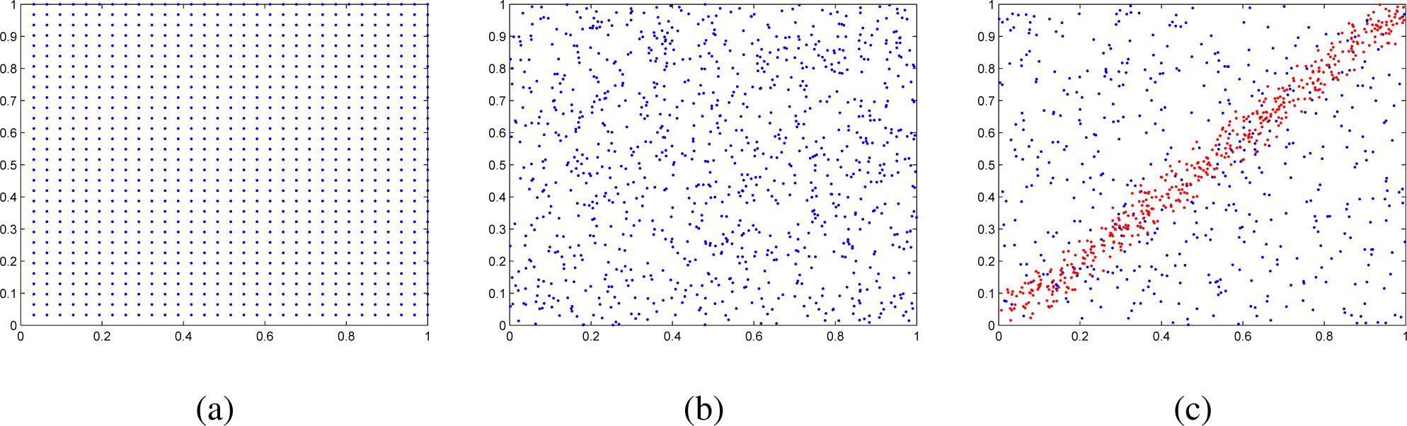
For illustrative purposes, we considered three different scenarios of point patterns. In the first scenario, we considered a set of 961 spatial points distributed on a regular grid 31 × 31 (Figure 2a). In the second scenario, we simulated N = 1000 realizations from a uniform distribution (Figure 2b), and in the third scenario, we simulated N1 = 500 points from a uniform distribution and N2 = 500 points along a linear pattern with a slope of 45 degrees (Figure 2c). Further examples could be considered with a slope ranging between zero and 180 degrees as in [34].
Figure 3 represents the directional multiscale wavelet entropy for the three datasets in Figure 2. In the first case, the entropy is approximatively equal to zero for each direction and for each scale. The higher values in the first level of resolution corresponding to the angles 0, 90 and 135 degrees are due to the border effects. In the second case (Figure 3b), the entropy seems higher in the first levels of resolution, but it is approximatively equal for each direction. In the third case, the entropy is higher in the area where the two random processes are superimposed, that is along the linear direction of 45 degrees.
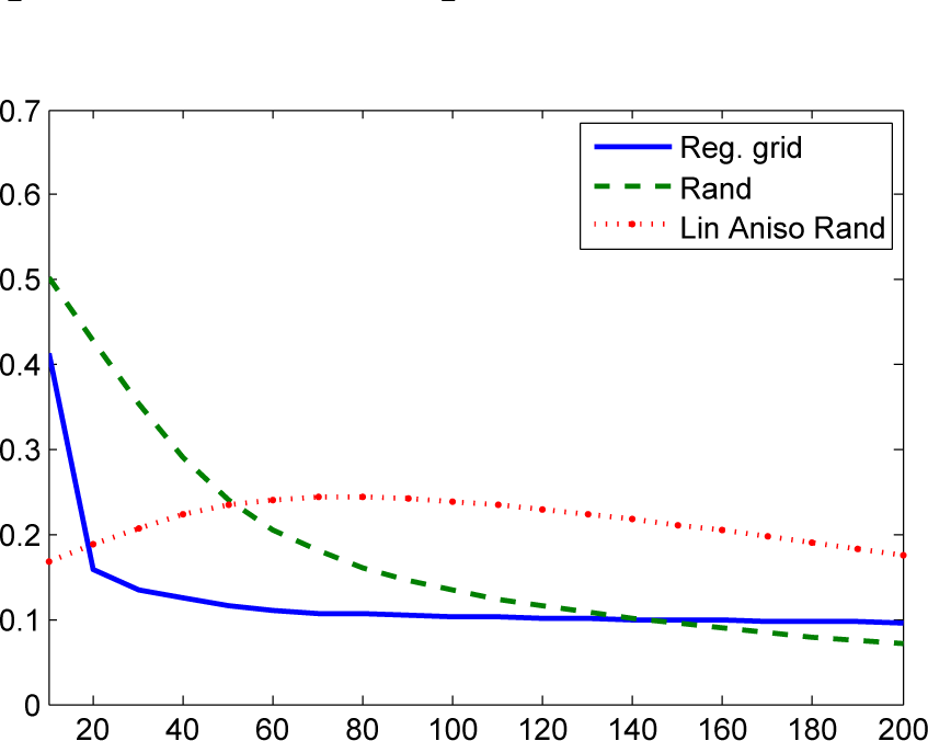
If we evaluate the entropy for each scale of resolution (Figure 4) using Equation (18), we observe that the entropy for the regular grid of points shows a fast decrease in the first levels of resolutions, while in the case of a random pattern, the entropy measure has a slower decay. A notably different behavior is shown when the process is generated from two different random processes, as in Figure 2. In this case, the entropy reaches its maximum value at a certain level of resolution.
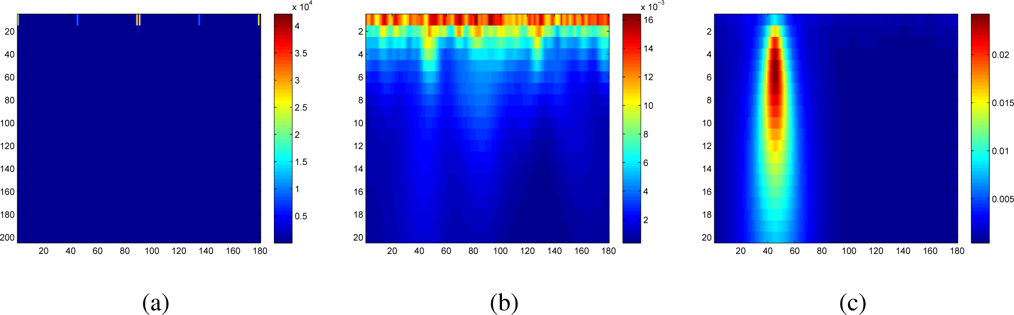
Figure 5 represents the spatial entropy for all directions and all scales for the three scenarios: low entropy for a regular grid (Figure 5a), high entropy for the random process (Figure 5b) and directional entropy for the superpositions of both patterns (Figure 5c).
Table 1 shows the global measure of wavelet entropy for the three scenarios. As expected, the first process given by points on a regular grid has the lowest entropy, while the third process resulting from the overlapping of two uniform distributions shows the highest entropy.
6. Application to Earthquake Data
We consider the Chilean earthquake catalog from January 2007 to August 2014, including 13,883 events with a magnitude larger than 3.0 and a depth less than 60 km. In order to show the spatial entropy, we focus on three main seismic areas represented in Figure 6. The first area (Figure 7a) is delimited by a rectangle with longitudes (−72, −79) and latitudes (−22.62, −18.62) and includes an earthquake event with magnitude 8.2 on 1 April 2014. The second zone (Figure 7b), including the town of Valparaiso, is delimited by coordinates with latitudes (−33.79, −29.79) and longitudes (−72, −69). Finally, the third area (Figure 7c), delimited by coordinates (−74.5, −71.5) and (−38.13, −34.13), includes a big earthquake (with magnitude 8.8) on 27 January 2010 in the town of Concepción. Although all areas extend along the Nazca plate, there are many other smaller faults along which earthquakes tend to cluster. The directional wavelet entropy can identify linear spatial directions with different entropy.
Figure 8 shows the wavelet entropy for each scale a and direction θ assessed on each dataset represented in Figure 7a–c, respectively. All plots show the maximum entropy along different dominant linear directions: 110 degrees for the first plot, 80 degrees for the second plot and 45 degrees for the third one. The entropy analysis through scales (Figures 9 and 10) shows the presence of different degrees of complexity at different scales. While Figures 9a and 9c indicate the maximum entropy in correspondence to a certain scale, in Figure 9b, the maximum entropy extends for a range of scales. The different behavior of Figure 9b is probably due to the source of its seismic events: unlike the events of Figures 7a and 7c, which are clustered along the main fault that caused their big earthquakes, Figure 7b shows different anisotropic clusters, probably due to the ruptures of independent faults.
If we consider the global (isotropic) spatial entropy as described by Equation (11), it is not possible to distinguish the main directions where the entropy tends to be the same. However, we can observe that the higher values of entropy are not concentrated close to the epicenters of the big events, where most likely the predictability is larger. This is confirmed by the analysis in Figure 11, which shows the directional multiscale entropy before (a) and after (b) the Iquique earthquake with a magnitude 8.2 occurring in the North of Chile on 1 April 2014. Although the entropy seems to be concentrated along a particular direction before the big earthquake, the uncertainty seems higher than the period after the M8.2 earthquake. Similar results are shown in Table 2 representing the global entropy for each area.
7. Conclusions
In this work, we have extended the concept of wavelet entropy to the two-dimensional case in order to detect the different complexity of a spatial point pattern. A new definition of wavelet entropy has been proposed for anisotropic processes using the directional Morlet wavelets. A simulation study has been used to show that the wavelet entropy is minimum when the process is a regular process, and it is maximum when the process is given by an overlapping of random point processes. Finally, an application to the earthquake catalog of Chile has been considered to detect the different spatial complexity. In particular, the results have shown that entropy is lower at spatial zones where a big earthquake happened than at areas characterized by different seismic activity, such as the area around the town of Valparaiso. Furthermore, the wavelet entropy is higher before a big earthquake than after. This means that aftershock events, which normally cluster along an active fault, have a lower degree of uncertainty than foreshock events, which are often characterized by a random distribution. The proposed methodology provides an important contribution to the study of earthquakes in Chile, given that it allows assessing the predictability of earthquakes in a given area.
Acknowledgments
The present work has been partially supported by Fondecyt Grant 1131147 from the Chilean government and by Grants MTM2013-43917-P and P1-1B2012-52.
Author Contributions
All authors have contributed to the study and preparation of the article. All authors have read and approved the final manuscript.
Conflicts of Interest
The authors declare no conflict of interest.
References
- Clausius, R. On the Motive Power of Heat, and on the Laws which may be Deduced from it for the Theory of Heat. Ann. Phys. 1850, 20, 2010. [Google Scholar]
- Boltzmann, L. Einige Allgemeine Satze Iiber Warmegleichgewicht unter Gas-molekulen. Sitzungsber. Akad. Wiss. Wien 1871, 63, 679–711. [Google Scholar]
- Shannon, C. A Mathematical Theory of Communication. Bell Syst. Tech. J 1948, 27, 379–423. [Google Scholar]
- Sengupta, B.; Stemmler, M.B.; Friston, K.J. Information and Efficiency in the Nervous System-A Synthesis. PLoS Comput. Biol 2013, 9. [Google Scholar] [CrossRef]
- Wong, A.K.C.; Sahoo, P.K. A Gray Level Threshold Selection Method Based on Maximum Entropy Principle. IEEE Trans. Syst. Man. Cybern 1989, 19, 866–871. [Google Scholar]
- Zhang, Y.; Wu, L. Optimal Multi-Level Thresholding Based on Maximum Tsallis Entropy via an Artificial Bee Colony Approach. Entropy 2011, 13, 841–859. [Google Scholar]
- Oladipo, E.O. Spectral Analysis of Climatological Time Series: On the Performance of Periodogram, Non-integer and Maximum Entropy Methods. Theor. Appl. Climatol 1988, 39, 40–53. [Google Scholar]
- Koutsoyiannis, D. Uncertainty Entropy Scaling and Hydrological Stochastics, 2, Time Dependence of Hydrological Processes and time Scaling. Hydrol. Sci. J 2005, 50, 405–426. [Google Scholar]
- Li, S.; Zhou, Q.; Wu, S.; Dai, E. Measurement of Climate Complexity Using Sample Entropy. Int. J. Climatol 2006, 26, 2131–2139. [Google Scholar]
- AghaKouchak, A. Entropy-Copula in Hydrology and Climatology. J. Hydrometeorol 2014, 15, 2176–2189. [Google Scholar]
- Nicholson, T.; Sambridge, M.; Gudmundsson, O. On Entropy and Clustering in Earthquake Hypocentre Distributions. Geophys. J. Int 2000, 142, 37–51. [Google Scholar]
- Telesca, L.; Lapenna, V.; Lovallo, M. Information Entropy Analysis of Seismicity of Umbria-Marche Region (Central Italy). Nat. Hazards Earth Syst. Sci 2004, 4, 691–695. [Google Scholar]
- Telesca, L.; Lovallo, M.; Mohamed, A.E.E.A.; ElGabry, M.; El-hady, S.; Abou Elenean, K.M.; ElBary, R.E.F. Informational Analysis of Seismic Sequences by Applying the Fisher Information Measure and the Shannon Entropy: An Application to the 2004–2010 Seismicity of Aswan Area (Egypt). Physica A 2012, 391, 2889–2897. [Google Scholar]
- Telesca, L.; Lovallo, M.; Babayev, G.; Kadirov, F. Spectral and Informational Analysis of Seismicity: An Application to the 1996–2012 Seismicity of the Northern Caucasus-Azerbaijan Part of the Greater Caucasus-Kopet Dag Region. Physica A 2013, 392, 6064–6078. [Google Scholar]
- Telesca, L.; Lovallo, M.; Chamoli, A.; Dimri, V.P.; Srivastava, K. Fisher-Shannon Analysis of Seismograms of Tsunamigenic and Non-tsunamigenic Earthquakes. Physica A 2013, 392, 3424–3429. [Google Scholar]
- Telesca, L.; Lovallo, M.; Martí Molist, J.; Lopez Moreno, C.; Abella Mendelez, R. Using the Fisher-Shannon Method to Characterize Continuous Seismic Signal during Volcanic Eruptions: Application to 2011–2012 El Hierro (Canary Islands) Eruption. Terra Nova 2014, 26, 425–429. [Google Scholar]
- Rényi, A. On Measures of Entropy and Information, Proceedings of the 4th Berkeley Symposium on Mathematics, Statistics and Probability, Berkeley, CA, USA, 20 June–30 July 1960; Neyman, Jerzy, Ed.; Berkeley: New York, NY, USA, 1961; pp. 547–561.
- Papoulis, A. Probability, Random Variables and Stochastic Processes; McGraw-Hill: New York, NY, USA, 1984. [Google Scholar]
- Telesca, L.; Cuomo, V.; Lapenna, V.; Macchiato, M. Statistical Analysis of Fractal Properties of Point Processes Modelling Seismic Sequences. Phys. Earth Planet. Int 2001, 12, 65–83. [Google Scholar]
- Labat, D. Recent Advances in Wavelet Analyses: Part 1. A review of Concepts. J. Hydrol 2005, 314, 275–288. [Google Scholar]
- Rosso, O.; Blanco, S.; Yordanowa, J.; Kolev, V.; Figliola, A.; Schürmann, M.; Ba¸sar, E. Wavelet Entropy: A New Tool for Analysis of Short Duration Brain Electrical Signals. J. Neurosci. Methods 2001, 105, 65–75. [Google Scholar]
- Sello, S. Wavelet Entropy and the Multi-peaked Structure of Solar Cycle Maximum. New Astron 2003, 8, 105–117. [Google Scholar]
- Perez, D.G.; Zunino, L.; Garavaglia, M.; Rosso, O.A. Wavelet Entropy and Fractional Brownian Motion Time Series. Physica A 2006, 365, 282–288. [Google Scholar]
- Zunino, L.; Perez, D.G.; Garavaglia, M.; Rosso, O.A. Wavelet Entropy of Stochastic Processes. Physica A 2007, 379, 503–512. [Google Scholar]
- Lyubushin, A. Prognostic Properties of Low-Frequency Seismic Noise. Nat. Sci 2012, 4, 659–666. [Google Scholar]
- Lyubushin, A. How Soon would the next Mega-Earthquake Occur in Japan? Nat. Sci 2013, 5, 1–7. [Google Scholar]
- Donoho, D.L. Nonlinear Wavelet Methods for Recovery of Signals Densities Spectra from Indirect and Noisy Data. In Proceedings of Symposia in Applied Mathematics; American Mathematical Society; Washington, WA, USA, 1993; pp. 173–205. [Google Scholar]
- Gao, W.; Li, B.L. Wavelet Analysis of Coherent Structures at the Atmosphere-Forest Interface. J. Appl. Meteorol 1993, 32, 1717–1725. [Google Scholar]
- Grenfell, N.; Bjørnstad, B.T.O.; Kappey, J. Travelling Waves and Spatial Hierarchies in Measles Epidemics. Nature 2001, 414, 716–723. [Google Scholar]
- Saunders, S.C.; Chen, J.; Crow, T.R.; Brofoske, K.D. Hierarchical Relationships between Landscape Structure and Temperature in a Managed Forest Landscape. Landsc. Ecol 1998, 13, 381–395. [Google Scholar]
- Brosofske, K.D.; Chen, J.; Crow, T.R.; Saunders, S.C. Vegetation Responses to Landscape Structure at Multiple Scales across a Northern Wisconsin, USA, Pine Barrens Landscape. Plant Ecol 1999, 143, 203–318. [Google Scholar]
- Harper, K.A.; Macdonald, S.E. Structure and Composition of Riparian Boreal Forest: New Methods for Analyzing Edge Influence. Ecology 2001, 82, 649–659. [Google Scholar]
- Perry, J.N.; Liebhold, A.M.; Rosenberg, M.S.; Dungan, J.; Miriti, M.; Jakomulska, A.; Citron-Pousty, S. Illustrations and Guidelines for Selecting Statistical Methods for Quantifying Spatial Pattern in Ecological Data. Ecography 2002, 25, 578–600. [Google Scholar]
- Mateu, J.; Nicolis, O. Multiresolution Analysis of Linearly-Oriented Spatial Point Patterns. J. Stat. Comput. Simul 2015, 8, 621–637. [Google Scholar]
- Goodall, D.W. Some Considerations in the Use of Point Quadrats for the Analysis of Vegetation. Aust. J. Sci. Res. B 1952, 5, 1–41. [Google Scholar]
- Matérn, B. Spatial Variation: Stochastic Models and their Application to some Problems in Forest Surveys and other Sampling Investigations. Esselte 1960, 49, 5. [Google Scholar]
- Matérn, B. Spatial Variation, 2nd ed; Springer: Berlin, Germany, 1986. [Google Scholar]
- Ripley, B.D. Spatial Statistics; Wiley: New York, NY, USA, 1981. [Google Scholar]
- Neyman, J.; Scott, E.L. Statisical Approach to Problems of Cosmology. J. R. Stat. Soc. B 1958, 20, 1–43. [Google Scholar]
- Cliff, A.D.; Ord, J.K. Spatial Processes: Models and Applications; Pion: London, UK, 1981. [Google Scholar]
- Ogata, Y. Space-Time Point Process Models for Earthquake Occurrences. Ann. Inst. Stat. Math 1998, 50, 379–402. [Google Scholar]
- Diggle, P.J.; Richardson, S. Epidemiological Studies of Industrial Pollutants: An Introduction. Int. Stat. Rev 1993, 61, 203–206. [Google Scholar]
- Stoyan, D.; Kendall, W.; Mecke, J. Stochastic Geometry and its Applications, 2nd ed; Wiley: Chichester, UK, 1995. [Google Scholar]
- Diggle, P.J. Statistical Analysis of Spatial Point Patterns; Hodder Education: London, UK, 2003. [Google Scholar]
- Baddeley, A.; Gregori, P.; Mateu, J.; Stoica, R.; Stoyan, D. (Eds.) Case Studies in Spatial Point Process Modeling (Lecture Notes in Statistics); Springer: Berlin, Germany, 2006.
- Illian, J.; Penttinen, A.; Stoyan, H.; Stoyan, D. Statistical Analysis and Modeling of Spatial Point Patterns; Wiley: Chichester, UK, 2008. [Google Scholar]
- Gelfand, A.E.; Diggle, P.J.; Fuentes, M.; Guttorp, P. (Eds.) Handbook of Spatial Statistics; CRC Press: Boca Raton, FL, USA, 2010.
- Ohser, J.; Stoyan, D. On the Second-Order and Orientation Analysis of Planar Stationary Point Processes. Biometr. J 1981, 23, 523–533. [Google Scholar]
- Stoyan, D.; Benes, V. Anisotropy Analysis for Particle Systems. J. Microsc 1991, 164, 159–168. [Google Scholar]
- Mateu, J. Second-Order Characteristics of Spatial Marked Processes with Applications. Nonlinear Anal. R. World Appl 2000, 1, 145–162. [Google Scholar]
- Redenbach, C.; Särkkä, A.; Freitag, J.; Schladitz, K. Anisotropy Analysis of Pressed Point Processes. Adv. Stat. Anal 2009, 93, 237–261. [Google Scholar]
- Møller, J.; Rasmussen, J.G. A Sequential Point Process Model and Bayesian Inference for Spatial Point Patterns with Linear Structures. Scand. J. Stat 2012, 39, 618–634. [Google Scholar]
- Telesca, L.; Lovallo, M.; Golay, J.; Kanevski, M. Comparing Seismicity Declustering Techniques by Means of the Joint Use of Allan Factor and Morisita Index. Stoch. Environ. Res. Risk Assess 2015. [Google Scholar] [CrossRef]
- Schenk, H.J.; Mahall, B.E. Positive and Negative Interactions Contribute to a North-South-Patterned Association between two Desert Shrub Species. Oecologia 2002, 132, 402–410. [Google Scholar]
- Rosenberg, M.S. Wavelet Analysis for Detecting Anisotropy in Point Patterns. J. Veg. Sci 2004, 15, 277–284. [Google Scholar]
- Blanco, S.; Figliola, A.; Quiroga, R.Q.; Rosso, O.A.; Serrano, E. Time-Frequency Analysis of Electroencephalogram Series. III. Wavelet Packets and Information Cost Function. Phys. Rev. E 1998, 57, 932–940. [Google Scholar]
- Vidakovic, B. Statistical Modeling by Wavelets; Wiley: New York, NY, USA, 1999. [Google Scholar]
- Mallat, S. A Wavelet Tour of Signal Processing; Academic Press: Waltham, MA, USA, 1999. [Google Scholar]
- Neupauer, R.M.; Powell, K.L. A Fully-Anisotropic Morlet Wavelet to Identify Dominant Orientations in a Porous Medium. Comput. Geosci 2005, 31, 465–471. [Google Scholar]
- Kumar, P. A Wavelet Based Methodology for Scale-Space Anisotropic Analysis. Geophys. Res. Lett 1995, 22, 2777–2780. [Google Scholar]
- Brillinger, D. Some Wavelet Analyses of Point Process Data, Proceedings of the Thirty-First Asilomar Conference on Signals, Systems and Computers; IEEE, 1–4 November 1998; Universidade de Sao Paulo: Brazil; pp. 1087–1091.
- Nicolis, O. Spatio-Temporal Analysis of Earthquake Occurrences Using a Multiresolution Approach, Mathematics of Planet Earth Lecture Notes in Earth System Sciences; Springer: Berlin, Heidelberg, Germany, 2014; pp. 179–183.
Figure 1.
Fully-anisotropic directional Morlet wavelet with parameters: (a) D = 0.8, k0 = 5.5, θ = 30; (b) D = 0.1, k0 = 5.5, θ = 90.
Figure 1.
Fully-anisotropic directional Morlet wavelet with parameters: (a) D = 0.8, k0 = 5.5, θ = 30; (b) D = 0.1, k0 = 5.5, θ = 90.
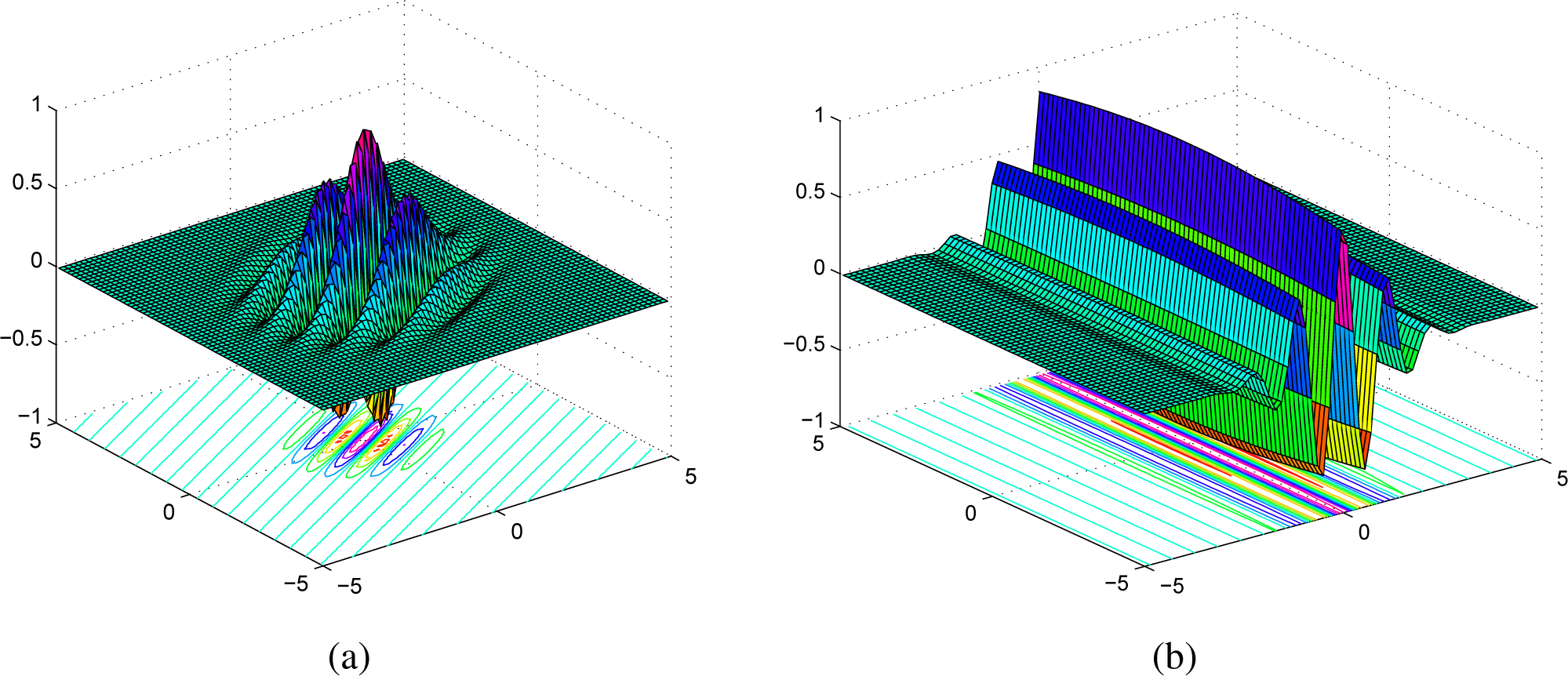
Figure 2.
(a) Spatial points on a regular grid of size 31 × 31 ; (b) simulated spatial points (n = 1000) from a uniform distribution U[0, 1]; (c) simulated spatial points using a uniform distribution U[0, 1] with n = 500 and an overlapped simulated linear pattern generated by a uniform distribution U[0, 1] with n = 500 along the line with a slope of 45 degrees.

Figure 3.
(a) Directional multiscale wavelet entropy for the: regular grid; (b) set of random points; (c) set of random points with a linear pattern.
Figure 3.
(a) Directional multiscale wavelet entropy for the: regular grid; (b) set of random points; (c) set of random points with a linear pattern.

Figure 4.
Multiscale wavelet entropy for the: regular grid (blue line); set of random points (green dashed line); set of random points with a linear pattern overlapped (red points).
Figure 4.
Multiscale wavelet entropy for the: regular grid (blue line); set of random points (green dashed line); set of random points with a linear pattern overlapped (red points).

Figure 5.
(a) Spatial wavelet entropy for the: regular grid; (b) set of random points; (c) set of random points with a linear pattern overlapped.
Figure 5.
(a) Spatial wavelet entropy for the: regular grid; (b) set of random points; (c) set of random points with a linear pattern overlapped.
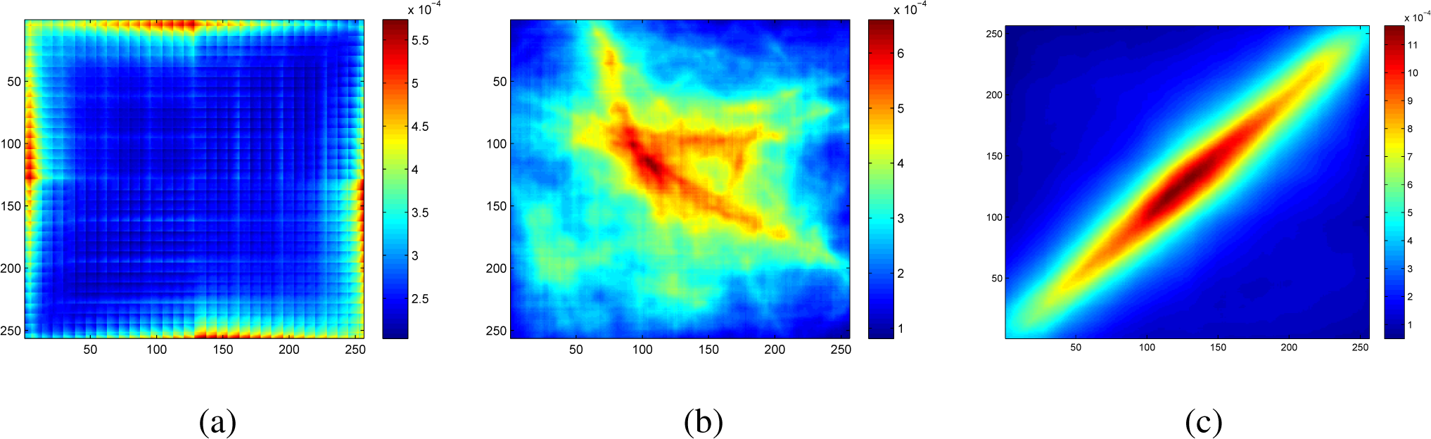
Figure 6.
Earthquake catalog of Chile form January 2007 to August 2014 with a depth less than 60 km and a minimum magnitude of 3.0; red rectangles indicate three important seismic areas.
Figure 6.
Earthquake catalog of Chile form January 2007 to August 2014 with a depth less than 60 km and a minimum magnitude of 3.0; red rectangles indicate three important seismic areas.
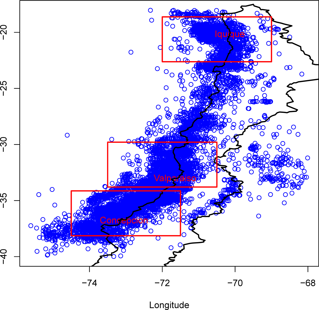
Figure 7.
Earthquakes epicenters form January 2007 to August 2014 with a depth less than 60 km and a minimum magnitude of 3.0 for three areas of Chile: (a) the first area located in the North of Chile, including the town of Iquique, is delimited by latitudes (−22.62, −18.62) and longitudes (−72, −69); (b) the second area including the town of Valparaiso, is delimited by latitudes (−33.79, −29.79) and longitudes (−72, −69); (c) the third area including the town of Concepción, is delimited by latitudes (−38.14, −34.14) and longitudes (−74.5, −71.5).
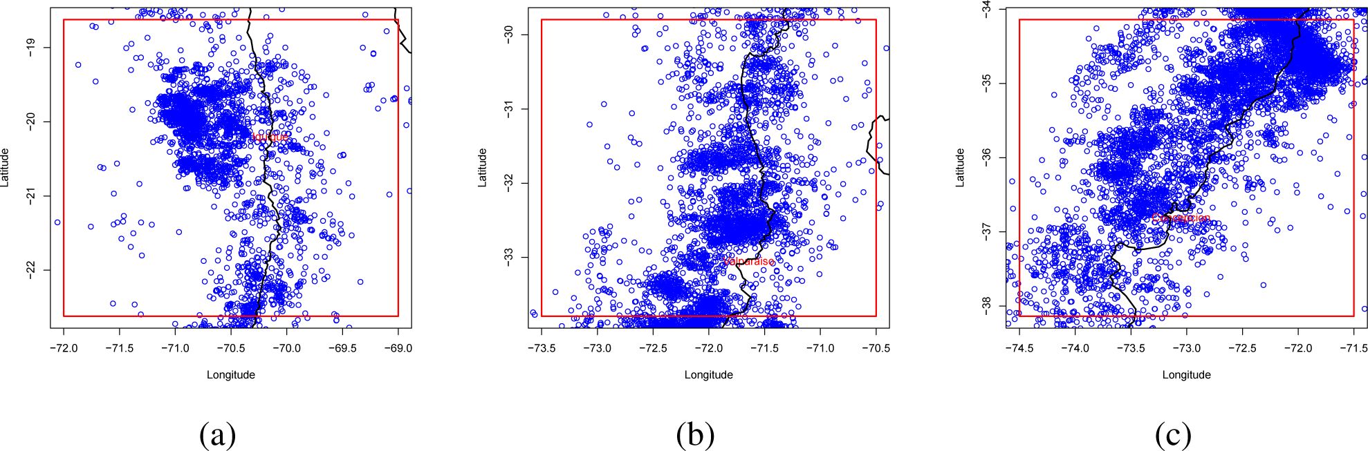
Figure 8.
Directional multiscale wavelet entropy for the epicenters for each area of Figure 7.
Figure 8.
Directional multiscale wavelet entropy for the epicenters for each area of Figure 7.
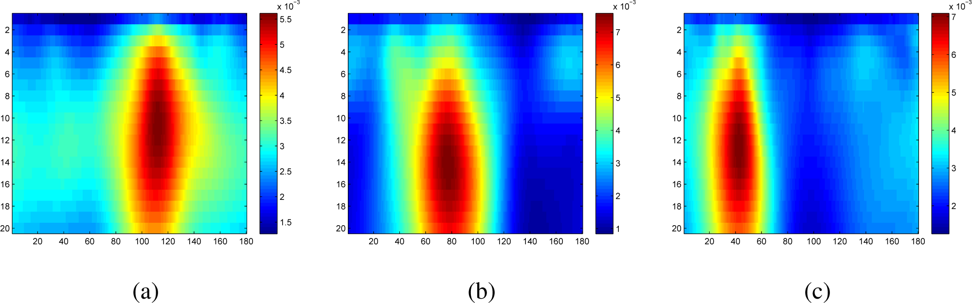
Figure 9.
Wavelet entropy for each scale a and for all directions θ for three areas: (a) the area delimited by latitudes (−22.62, −18.62) and longitudes (−72, −69); (b) the area delimited by latitudes (−33.79, −29.79) and longitudes (−72, −69); (c) the area including the town of Concepción delimited by latitudes (−38.14, −34.14) and longitudes (−74.5, −71.5).
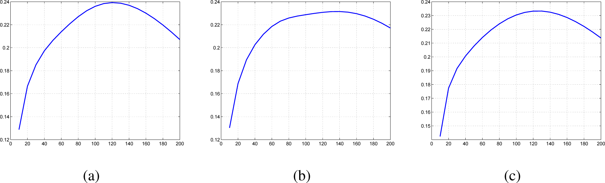
Figure 10.
Spatial wavelet entropy for three areas: (a) the area delimited by latitudes (−22.62, −18.62) and longitudes (−72, −69); (b) the area delimited by latitudes (−33.79, −29.79) and longitudes (−72, −69); (c) the area, including the town of Concepción, delimited by latitudes (−38.14, −34.14) and longitudes (−74.5, −71.5).

Figure 11.
Wavelet entropy for each scale a and for each angle θ for the earthquake events before (a) and after (b) the Iquique earthquake occurring on 1 April 2014.
Figure 11.
Wavelet entropy for each scale a and for each angle θ for the earthquake events before (a) and after (b) the Iquique earthquake occurring on 1 April 2014.


Table 1.
Global entropy for the three processes: (a) spatial points on a regular grid of size 31 × 31; (b) simulated spatial points (n = 1000) from a uniform distribution U[0, 1]; (c) simulated spatial points using a uniform distribution U[0, 1] with n = 500 together with an overlapped linear pattern generated by a uniform distribution U[0, 1] with n = 500 along the line y = x.
| Wavelet Entropy | |
|---|---|
| Regular | 2.47 |
| Random | 3.60 |
| Random + linear | 4.30 |
Table 2.
Global entropy for the earthquake catalog of Chile: “Window 1”, “Window 2” and “Window 3” represent the wavelet entropy for the events in the rectangular windows represented in Figures 7a, 7b and 7c, respectively. The last two rows show the entropy values for the period before the Iquique earthquake and after the Iquique earthquake.
| Wavelet Entropy | |
|---|---|
| Window 1 | 4.30 |
| Window 2 | 4.55 |
| Window 3 | 4.30 |
| Window 1 (before) | 4.31 |
| Window 1 (after) | 4.29 |
© 2015 by the authors; licensee MDPI, Basel, Switzerland This article is an open access article distributed under the terms and conditions of the Creative Commons Attribution license (http://creativecommons.org/licenses/by/4.0/).
Share and Cite
MDPI and ACS Style
Nicolis, O.; Mateu, J. 2D Anisotropic Wavelet Entropy with an Application to Earthquakes in Chile. Entropy 2015, 17, 4155-4172. https://doi.org/10.3390/e17064155
AMA Style
Nicolis O, Mateu J. 2D Anisotropic Wavelet Entropy with an Application to Earthquakes in Chile. Entropy. 2015; 17(6):4155-4172. https://doi.org/10.3390/e17064155
Chicago/Turabian StyleNicolis, Orietta, and Jorge Mateu. 2015. "2D Anisotropic Wavelet Entropy with an Application to Earthquakes in Chile" Entropy 17, no. 6: 4155-4172. https://doi.org/10.3390/e17064155