A Mean-Variance Hybrid-Entropy Model for Portfolio Selection with Fuzzy Returns

Abstract

In this paper, we define the portfolio return as fuzzy average yield and risk as hybrid-entropy and variance to deal with the portfolio selection problem with both random uncertainty and fuzzy uncertainty, and propose a mean-variance hybrid-entropy model (MVHEM). A multi-objective genetic algorithm named Non-dominated Sorting Genetic Algorithm II (NSGA-II) is introduced to solve the model. We make empirical comparisons by using the data from the Shanghai and Shenzhen stock exchanges in China. The results show that the MVHEM generally performs better than the traditional portfolio selection models.

1. Introduction

The financial market is a complex system, in which investors need to make a tradeoff between return and risk in an uncertain environment. Modern portfolio theory was first proposed in 1952 by Markowitz [1], who put forward the classic mean-variance model (MVM) as also created a precedent for the use of quantitative methods in investment portfolio selection. MVM has been proved effective and useful, but its disadvantages such as “corner solutions”, low diversity and poor out-of-sample performance should not be ignored. Many subsequent researchers have rewritten and developed the model with new methods or new elements to get better results.

Recently, portfolio selection problems have been studied under fuzzy environment conditions. For example, Watada [2] proposed a portfolio selection model in which expected return and risk are objectives, and S-type membership functions characterize levels of satisfaction. Ostermark [3] applied the principle of fuzzy decision in portfolio objectives and constraints, and then proposed a similar dynamic portfolio management model. Li et al. [4] combined fuzzy simulation with hybrid intelligent algorithm, and solved the mean-variance-skewness model for a fuzzy environment scenario. Doumpos et al. [5] presented some fuzzy models for selecting portfolios considering different approaches for quantifying the uncertainty of future returns. Zhang et al. [6] proposed a new fuzzy programming approach for multi-period portfolio optimization subject to return demand and risk control.

With regard to portfolio risk measurement, a number of portfolio models have been proposed, such as the semi-variance model (see Markowitz [7]), the absolute deviation model (see Konno [8]), the maximum loss minimization model (see Young [9]), the maximum absolute deviation model (see Cai [10]), the lower partial moment model (see Bawa [11]), the mean-variance-skewness model (see Jana [12]) and the like. Yu et al. [13] pointed out that different risk measurement models lead to significant different impacts on portfolio structures. Moreover, Zhou [14] found that entropy, as a valid measure of uncertainty, has been more and more widely used in the financial field, and its effectiveness in portfolio selection has also been confirmed by many scholars. Philippatos and Wilson [15] were the first to introduce the concept of entropy to portfolio selection. The mean-entropy model (MEM) and the mean relative-entropy model (MREM) they proposed have become the foundations for research in this area. Cheng [16] proposed a relative-entropy-based risk measurement. Ou [17] came up with an extension of entropy, which could describe the growth rate of the capital upon receiving new information, and obtain the optimal investment ratio. Bera [18] proposed to use cross entropy measure. Huang [19] developed a simple and effective algorithm for the calculation of MEM’s efficient boundaries and established a new model: fuzzy mean-entropy model. Usta and Kantar [20] compared the mean-variance-skewness-entropy model with the classic models, and found that the models with entropy factor performed the best in out-of-sample tests. De Luca and Termini were the first to come up with the concept of a hybrid entropy which was called total entropy. Based on hybrid entropy, Xu et al. [21] estimated asset risk resulting from joint randomness and fuzziness. Yu et al. [22] compared the mean–variance efficiency, realized portfolio values, and diversity of the models incorporating different entropy measures and found that Yager’s entropy yielded higher performance. Zhou [23] and Zhang [24] introduced other entropy-related models such as incremental entropy-skewness model and possibilistic mean semivariance-entropy model.

In this paper, we propose the MVHEM based on fuzzy returns for portfolio selection in which we define portfolio return as fuzzy average yield and risk as mixed hybrid entropy and variance, respectively. Several empirical comparisons based on Chinese stock markets are given to illustrate the effectiveness of the proposed model. The rest of this paper is organized as follows: in Section 2, we first introduce some basic knowledge about fuzzy variables and hybrid entropy, then combine the MVM and MEM and propose the MVHEM. We also provide an algorithm to solve the optimization problem. Several empirical comparisons are given among the MVHEM, MVM and MEM in Section 3. Section 4 summarizes our work.

2. Mean-Variance Hybrid-Entropy Portfolio Optimization Model

2.1. Fuzzy Returns Predicted by the Markov Method

2.1.1. The Expected Value and Variance of the Triangular Fuzzy Returns

Suppose that ξ = (a, b, c) is a triangular fuzzy variable with the following membership function:

$$\mu (x)=\{\begin{array}{c}\left(x-a\right)/\left(b-a\right),\mathrm{if}a\le x\le b,\\ \left(x-c\right)/\left(b-c\right),\mathrm{if}b\le x\le c,\\ 0,otherwise\end{array}$$

(1)

According to the Credibility Measure Theory (see Liu [25]), the expected value and variance of the triangular fuzzy returns of stocks are given by:

$$E\left[\xi \right]=\frac{a+2b+c}{4}$$

(2)

$$V\left[\xi \right]=\frac{33{\mathrm{\alpha }}^3+21{\mathrm{\alpha }}^2\mathrm{\beta }+11{\mathrm{\alpha }\mathrm{\beta }}^2-{\mathrm{\beta }}^3}{384\mathrm{\alpha }}$$

(3)

where α = max {b – a, c − b}, β = min{b – a, c – b}. Especially, if b – a = c – b, we have $V\left[\xi \right]=\frac{\left(b-a\right)2}{6}$.

Based on the Zedeh Extension Principle, when ${\tilde{r}}_i=(a_i,r_i,b_i)(i=1,2,\dots ,n)$ are all triangular fuzzy variables, ${\displaystyle {\sum }_{i=1}^n{\tilde{r}}_i{x}_i=({\displaystyle {\sum }_{i=1}^n{x}_i{a}_i,{\displaystyle {\sum }_{i=1}^n{x}_i{r}_i,{\displaystyle {\sum }_{i=1}^n{x}_i{b}_i}}})}$ are triangular fuzzy variables as well. Therefore, we get:

$$E\left[{\tilde{r}}_1{x}_1+{\tilde{r}}_2{x}_2+\cdots +{\tilde{r}}_n{x}_n\right]={\displaystyle {\sum }_{i=1}^n(a_i+2r_i+b_i)x_i/4}$$

(4)

$$\begin{array}{l}V[{\tilde{r}}_1{x}_1+{\tilde{r}}_2{x}_2+\cdots +{\tilde{r}}_n{x}_n]\\ =\frac{11{({\displaystyle {\sum }_{i=1}^n{x}_i(b_i-a_i)})}^2|{\displaystyle {\sum }_{i=1}^n{x}_i(2r_i-a_i-b_i)|}}{192\left({\displaystyle {\sum }_{i=1}^n{x}_i(b_i-a_i)+|{\displaystyle {\sum }_{i=1}^n{x}_i(2r_i-a_i-b_i)}|}\right)}\\ +\frac{2(8{\displaystyle {\sum }_{i=1}^n{x}_i(b_i-a_i)+3|{\displaystyle {\sum }_{i=1}^n{x}_i}(2r_i-a_i-b_i)|})({\left({\displaystyle {\sum }_{i=1}^n{x}_i(b_i-a_i)}\right)}^2+{({\displaystyle {\sum }_{i=1}^n{x}_i(r_i-a_i)})}^2}{192\left({\displaystyle {\sum }_{i=1}^n{x}_i(b_i-a_i)+|{\displaystyle {\sum }_{i=1}^n{x}_i(2r_i-a_i-b_i)}|}\right)}\end{array}$$

(5)

2.1.2. Prediction of Stock Returns

Taking randomness and fuzziness of stock price volatility into consideration, stock yields are set as triangular fuzzy random variables. Then let ${\tilde{r}}_i$ be the return rate of stock i, ${\tilde{r}}_i=(a_i,r_i,b_i)$, i = 1,2, …, n. Let r_i denote the mathematical expectation of the random variable of ${\tilde{r}}_i$; b_i and a_i are the ceiling return and the floor return, respectively. Hence, the membership function of ${\tilde{r}}_i$ is defined by the following functions:

$$\mu (x)=\{\begin{array}{c}(x-a_i)/(r_i-a_i),\mathrm{if}{a}_i\le x\le r_i\\ (x-b_i)/(r_i-b_i),\mathrm{if}{r}_i\le x\le b_i\\ 0,\text{otherwise}\end{array}$$

(6)

Next, we use the Markov method to predict the fuzzy returns of stock following steps as below:

• Step 1. Collect the historical trading data in a sample period (in this paper, it is one year or three years), including the opening price R_t1, closing price R_t2, ceiling price R_t3 and floor price R_t4, t = 1,2, …, N, where N is the number of sub-intervals. Then we calculate the possible average rates of returns $r_{te}=\frac{R_{t2}-R_{t1}}{R_{t1}}$, the highest possible rates of returns $r_{th}=\frac{R_{t2}-R_{t1}}{R_{t1}}$, and the lowest possible rates of returns $r_{tl}=\frac{R_{t4}-R_{t1}}{R_{t1}}$.
• Step 2. Use the classic K-Means cluster analysis method to get the step transition matrix. We divide the range of rate of return into M intervals called state spaces and get mid-points d_i(i = 1,2, …, M) and probability p_ij(i, j = 1,2, …, M) that the return is in space j if it was in space i the last state. Then form one step transition matrix by these probabilities:

$$\mathrm{P}=\left(\begin{array}{c}{p}_{11}{p}_{12}\dots p_{1M}\\ p_{21}{p}_{22}\dots p_{2M}\\ \dots \\ p_{M1}{p}_{M2}\dots p_{MM}\end{array}\right)$$

(7)

• Step 3. Develop the state transition equation. The probability of stock return in state space i can be calculated by:

  $$\mathbf{x}=\mathit{Px}$$

  (8)

  where x = (x₁, x₂, …, x_M)^T, x₁, x₂, …, x_M ≥ 0, ${\displaystyle {\sum }_{i=1}^M{x}_i=1}$.
  The unique solution of the equation is x = (p₁, p₂, …, p_M)^T. Therefore the probabilities of the stock return in state space i after a long enough time are p₁, p₂, …, p_M.
• Step 4. Compute the prediction of the stock return by function $r={\displaystyle {\sum }_{i=1}^M{p}_i{d}_i}$. The highest possible rate of return r_th and lowest possible rate of return r_tl can be calculated in the same way. That is how we get the value of the ceiling return b_i and the floor return a_i. Hence, the prediction of our triangular fuzzy returns turns out to be ${\tilde{r}}_i=(a_i,r_i,b_i)$.

2.2. Hybrid Entropy

Hybrid entropy originated from Shannon entropy. Discrete Shannon entropy is referred to as the uncertainty of discrete random variable P in a probability space. That is:

$$S_n(P)=-{\displaystyle {\sum }_{i=1}^n{p}_i\ln p_i,{\displaystyle {\sum }_{i=1}^n{p}_i=1p_i\ge 0}}$$

(9)

Similarly, the uncertainty of discrete fuzzy random variable M in a fuzzy space can be expressed by De Luca-Termini [26] hybrid entropy as follows:

$$H_f(M)=H_f\left({\mathrm{\mu }}_1,{\mathrm{\mu }}_2,\dots ,{\mathrm{\mu }}_n\right)=-\frac{1}{n}{\displaystyle {\sum }_{i=1}^n\{{\mathrm{\mu }}_i{\log }_2{\mathrm{\mu }}_i+(1-{\mathrm{\mu }}_i){\log }_2\left(1-{\mathrm{\mu }}_i\right)\}}$$

(10)

Hybrid entropy is an effective tool to measure financial risk caused by both randomness and fuzziness simultaneously (Xu et al. [21]). The hybrid entropy is defined as:

$$H_h=-{\displaystyle {\sum }_{i=1}^n\{p_i{\mu }_i\log p_i{\mathrm{\mu }}_i+p_i(1-{\mathrm{\mu }}_i)\log p_i(1-{\mathrm{\mu }}_i)\}}$$

(11)

This H_h should meet the following requirements:

• H_h will reach its biggest value if and only if μ_i = 0.5 and p_i = 1/n (i = 1,2,…,n);
• H_h will reach its smallest value 0 if and only if μ_i = 0 or 1 (i = 1,2, …, n), p_i = 1 and p_j = 0(j ≠ i,i,j = 1,2,…,n);
• When randomness (ambiguity) disappears, hybrid entropy should be reduced to a normal probability entropy (fuzzy entropy).

Taking both the randomness and fuzziness of stock returns into consideration, we choose the discrete hybrid entropy to measure the risk of stock return.

2.3. Portfolio Optimization Model

In this section, we present the well-known traditional portfolio selection models and also develop a mean-variance hybrid-entropy model with fuzzy returns.

2.3.1. MVM and MEM

Markowitz’s MVM was the first risk measurement model to apply the mathematical methods into portfolio selection. In this model, mean measures the expected return and variance measures the risk. The two objectives of the investors are getting higher returns and lower risk relatively. The model is given as follows:

$$\mathrm{Min}{X}^{\mathrm{T}}CX\mathrm{s}.\mathrm{t}.\{\begin{array}{c}{\displaystyle {\sum }_{i=1}^N{x}_i{r}_i\ge c}\\ {\displaystyle {\sum }_{i=1}^N{x}_i=1;i=1,2,\dots ,\mathrm{n}}\end{array}$$

(12)

where the yield vector of N securities R = (r₁, r₂, …, r_N)^T; the wealth fraction invested in the securities X = (x₁, x₂, …, x_N)^T; C is the covariance matrix and c represents the given expected return.

But only taking advantage of variance to measure risk is not sufficient. That is why many scholars put forward the MEM, which uses the entropy instead of variance to measure the portfolio’s risk. The MEM is given as follows:

$$\mathrm{Max}f(x)={\displaystyle {\sum }_{i=1}^N{x}_i{r}_i\mathrm{Min}\mathrm{V}(x)={\displaystyle {\sum }_{i=1}^N{x}_i{h}_i\mathrm{s}.\mathrm{t}.}\{\begin{array}{c}{\displaystyle {\sum }_{i=1}^N{x}_i=1}\\ 0\le x_i\le \mu ,i=1,\dots ,\mathrm{n}\end{array}}$$

(13)

where the yield vector of N securities R = (r₁, r₂, …, r_N)^T the wealth fraction invested in the securities X = (x₁, x₂, …, x_N)^T, and the risk vector of N securities H = (h₁, h₂, …, h_N)^T.

2.3.2. MVHEM

We can see that the formula of hybrid entropy is improperly complex, and so is the hybrid entropy formula expressed by triangular fuzzy variables. The applicability will be greatly reduced if the model is too complex. Therefore, we use the approximate formula instead. The formula is:

$$H[{\tilde{r}}_1{x}_1+{\tilde{r}}_2{x}_2+\cdots +{\tilde{r}}_n{x}_n]={\displaystyle {\sum }_{i=1}^N{x}_i{H}_h({\tilde{r}}_i)}$$

(14)

Kalyagin et al. [27] once discussed the specifics of financial modeling and emphasized the multidimensional aspects of financial decisions, so here we choose multi-objective programming. This paper intends to measure the returns by the possibilistic mean of the fuzzy rate of return, and measure the risk by both variance and entropy, and thus form the mean-variance hybrid-entropy model for portfolio selection with fuzzy returns:

$$\begin{array}{l}\mathrm{Max}E[{\tilde{r}}_1{x}_1+{\tilde{r}}_2{x}_2+\cdots +{\tilde{r}}_n{x}_n]\\ \mathrm{Min}V[{\tilde{r}}_1{x}_1+{\tilde{r}}_2{x}_2+\cdots +{\tilde{r}}_n{x}_n]\\ \mathrm{Min}H({\tilde{r}}_1{x}_1+{\tilde{r}}_2{x}_2+\cdots +{\tilde{r}}_n{x}_n)={\displaystyle {\sum }_{i=1}^N{x}_i{H}_h({\tilde{r}}_i)}\\ \mathrm{s}.\mathrm{t}.\{\begin{array}{c}{\displaystyle {\sum }_{i=1}^N{x}_i=1}\\ x_1,x_2,\dots ,x_n\ge 0\end{array}\end{array}$$

(15)

MVHEM is a multi-objective optimization model. We use the improved algorithm NSGA-II proposed by Deb [28] to solve this optimization problem, which can effectively reduce the computational complexity.

Let $\mathrm{X}=\{x|{\displaystyle {\sum }_{i=1}^n{x}_i=1,x_i\ge 0,i=1,\dots ,n}\}$, $M^{+}=\underset{x\in X}{\max }M(x)$, $M^{-}=\underset{x\in X}{\min }M(x)$, $V^{+}=\underset{x\in X}{\max }V(x),V^{-}=\underset{x\in X}{\min }V(x),H^{+}=\underset{x\in X}{\max }H(x)$ and $H^{-}=\underset{x\in X}{\min }H(x)$. Then we could form a new multi-objective function as follows:

$$\begin{array}{l}\mathrm{Max}\frac{M(x)-M^{-}}{M^{+}-M^{-}}\\ \mathrm{Max}\frac{V(x)-V^{+}}{V^{-}-V^{+}}\\ \mathrm{Max}\frac{H(x)-H^{+}}{H^{-}-H^{+}}\\ \mathrm{s}.\mathrm{t}.\{\begin{array}{c}{\displaystyle {\sum }_{i=1}^N{x}_i=1}\\ x_1,x_2,\dots ,x_n\ge 0\end{array}\end{array}$$

(16)

which can be solved directly by MATLAB.

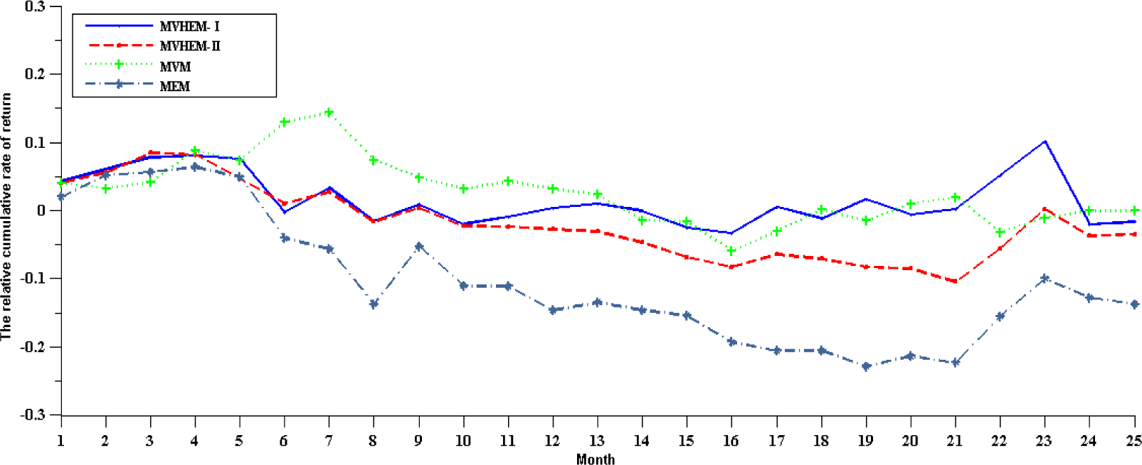
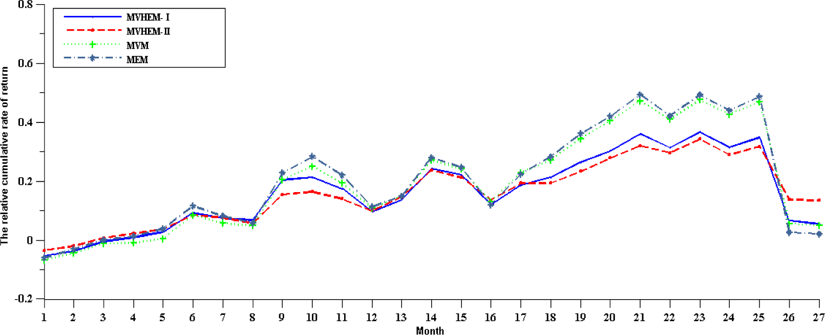
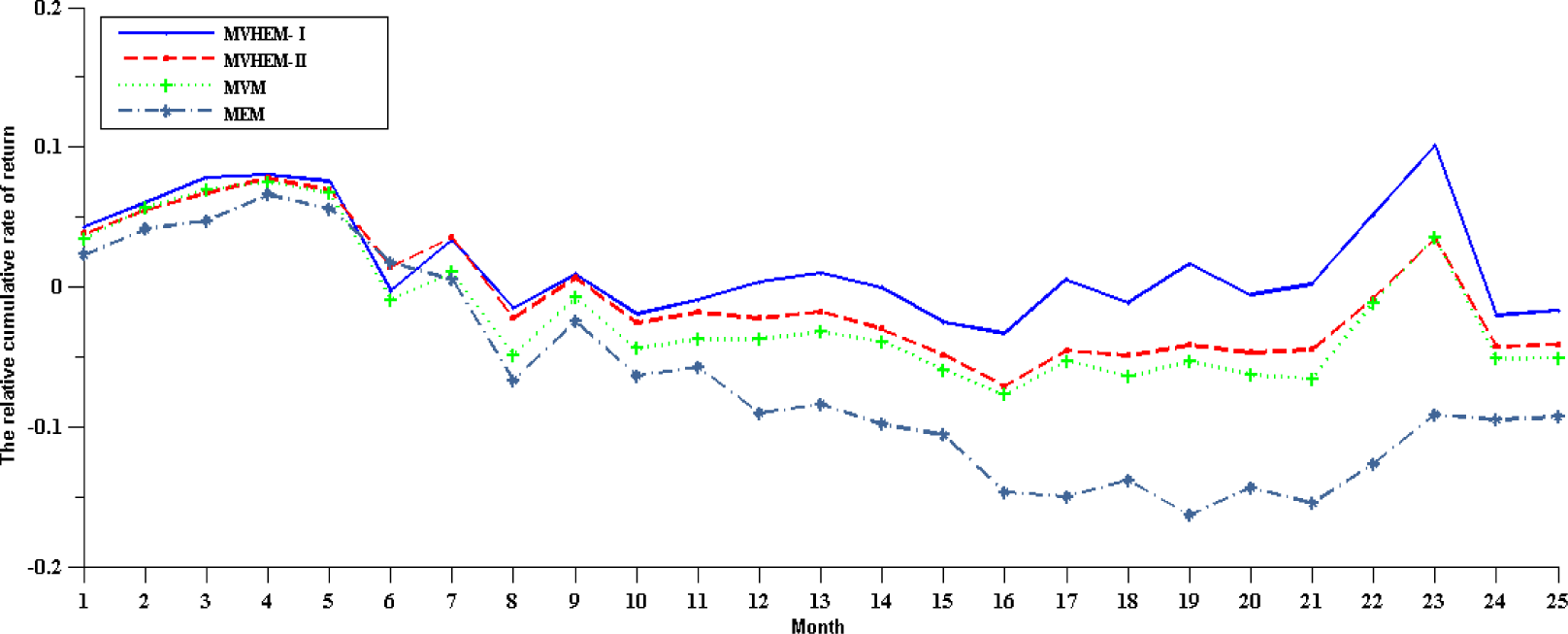
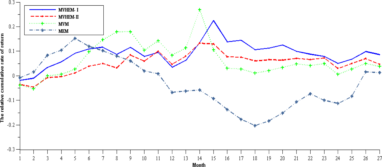
3. Empirical Comparisons

3.1. Sample Data

In order to avoid drastic fluctuations in portfolio returns which may result from industrial risk, we select 10 listed stocks from 10 different industries in Shanghai Stock Exchange (SHSE) and Shenzhen Stock Exchange (SZSE) in China, respectively. The original data obtained from the Straight Flush Software are one-year and three-year weekly data covering from 1 January in 2011 to 1 January in 2014, from which weekly yields, the highest possible yields and the lowest possible yields can be calculated. According to the Markov Method mentioned above, we obtain the prediction of stock returns as shown in

Table 1. The fuzzy returns of different sample period stocks in SHSE.

Sample Period	One-Year Period	Three-Year Period
Stock Code
600100	(−0.0314, 0.0070, 0.0494)	(−0.0398, −0.0042, 0.0391)
600270	(−0.0411, 0.0095, 0.0583)	(−0.0365, 0.0026, 0.4238)
600109	(−0.0433, 0.0009, 0.0496)	(−0.0441, 0.0027, 0.0464)
600664	(−0.0382, 0.0008, 0.0349)	(−0.0458, −0.0078, 0.0275)
600060	(−0.0445, 0.0045, 0.0527)	(−0.0418, 0.0018, 0.0450)
600714	(−0.0392, −0.0065, 0.0399)	(−0.0511, −0.0008, 0.0512)
600886	(−0.0351, −0.0043, 0.0353)	(−0.0321, −0.0025, 0.0277)
600638	(−0.0357, 0.0057, 0.0420)	(−0.0347, 0.0030, 0.0374)
600778	(−0.0354, −0.0031, 0.0362)	(−0.0414, −0.0009, 0.0389)
600081	(−0.0409, 0.0058, 0.0527)	(−0.0008, −0.0008, 0.0462)

and

Table 2. The fuzzy returns of different sample period stocks in SZSE.

Sample Period	One-Year Period	Three-Year Period
Stock Code
002186	(−0.0380, −0.0042, 0.0428)	(−0.0312,−0.0015,0.0313)
000791	(−0.0364, 0.0017, 0.0400)	(−0.0403, 0.0012, 0.0446)
002032	(−0.0329, 0.0031, 0.0444)	(−0.0382, −0.0026, 0.0351)
000002	(−0.0416, −0.0045, 0.0387)	(−0.0346, 0.0004, 0.0338)
000768	(−0.0357, 0.0045, 0.0513)	(−0.0347, −0.0005, 0.0414)
002226	(−0.0331, 0.0037, 0.0414)	(−0.0416, −0.0024, 0.0373)
300027	(−0.0598, 0.0284, 0.1017)	(−0.0466, 0.0055, 0.0579)
000088	(−0.0386, 0.0114, 0.0569)	(−0.0357, 0.0017, 0.0361)
300005	(−0.0531, 0.0025, 0.0549)	(−0.0488, −0.0020, 0.0464)
000001	(−0.0501, 0.0000, 0.0573)	(−0.0338, 0.0001, 0.0343)

.

From Tables 1 and 2, we can observe that compared to the one-year fuzzy returns, most of the three-year results display a trend of convergence, which means less volatility with shorter distance between the left endpoint and right endpoint, and the three-year fuzzy returns’ center point is much closer to zero.

Based on the fuzzy returns calculated and the Formulae (6) and (8), we have the possibilistic mean and the value of hybrid entropy of the sample stocks. The computational results are shown in

Table 3. Expected values and hybrid entropy calculated from different sample period stocks in SHSE.

Sample Period	One-Year Period		Three-Year Period
Stock Code	Expected Value	Hybrid Entropy	Expected Value	Hybrid Entropy
600100	0.0079	0.6303	−0.0023	0.6237
600270	0.0091	0.7088	0.0028	0.5525
600109	0.0020	0.5320	0.0019	0.5852
600664	−0.0004	1.0954	−0.0085	1.0520
600060	0.0043	0.6288	0.0017	0.4766
600714	−0.0031	0.6598	−0.0004	0.6944
600886	−0.0021	0.6981	−0.0023	0.6944
600638	0.0044	1.1528	0.0022	0.6767
600778	−0.0014	0.6217	−0.0011	0.5536
600081	0.0058	0.6796	0.0109	0.3789

and

Table 4. Expected values and hybrid entropy calculated from different sample period stocks in SZSE.

Sample Period	One-Year Period		Three-Year Period
Stock Code	Expected Value	Hybrid Entropy	Expected Value	Hybrid Entropy
002186	−0.0009	1.1940	−0.0007	1.0360
000791	0.0017	0.6555	0.0017	0.6981
002032	0.0044	1.1211	−0.0020	0.9846
000002	−0.0029	0.7656	0.0000	0.5124
000768	0.0061	0.5451	0.0014	0.3668
002226	0.0039	0.5890	−0.0023	1.1131
300027	0.0247	0.6167	0.0056	0.7336
000088	0.0103	1.1977	0.0009	0.7219
300005	0.0017	0.6466	−0.0016	0.9808
000001	0.0018	0.7208	0.0002	0.5996

.

It can be seen from Tables 3 and 4 that the three-year means are all smaller than the one-year means both in the SHSE and SZSE. Not all of the three-year sample’s hybrid entropy are smaller than the one-year sample’s, and we attribute this to the lack of fuzziness of the three-year sample, which affects the magnitude of the hybrid entropy to some extent.

3.2. The Empirical Comparisons among MVM, MEM and MVHEM

On the basis of the real historical data in Tables 1 and 2, we develop a portfolio model composed by ten stocks. The essence of this model is multi-objective. By using the NSGA-II, we get several Pareto optimal solutions for the stock portfolio. These optimal solutions can be divided into two categories: one category is income-oriented and focused on the pursuit of higher yields, the other is risk-oriented and focused on pursuing low risks. We single out one group from each type (MVHEM-I is income-oriented, and MVHEM-II is risk-oriented) as representations, and we also list results of two other classic models (MVM and MEM) for comparison. The results are shown in

Table 5. The proportion of one-year period sample stocks in different portfolio selection models in SHSE.

Stock Code	600100	600270	600109	600664	600060	600714	600886	600638	600778	600081
Model
MVHEM-I	0.2402	0.1574	0.1222	0.0359	0.1590	0.0378	0.0529	0.0416	0.0997	0.0535
MVHEM-II	0.0551	0.1067	0.0452	0.1804	0.2603	0.0544	0.0654	0.1907	0.0193	0.0220
MVM	0.1500	0.7054	0.0189	0.0012	0.0246	0.0053	0.0004	0.0459	0.0209	0.0281
MEM	0.9153	0.0019	0.0779	0.0002	0.0002	0.0005	0.0017	0.0002	0.0003	0.0008

Table 6. The proportion of three-year period sample stocks in different portfolio selection models in SHSE.

Stock Code	600100	600270	600109	600664	600060	600714	600886	600638	600778	600081
Model
MVHEM-I	0.0102	0.0916	0.0651	0.0231	0.0457	0.0741	0.0920	0.0690	0.0626	0.4650
MVHEM-II	0.0022	0.0795	0.0450	0.0149	0.0372	0.0500	0.4470	0.0582	0.0553	0.2090
MVM	0.0015	0.0294	0.0844	0.0000	0.1065	0.0003	0.0001	0.0272	0.0002	0.7490
MEM	0.0069	0.0565	0.0146	0.0062	0.0412	0.0147	0.1096	0.0514	0.0306	0.6672

Table 7. The proportion of one-year period sample stocks in different portfolio selection models in SZSE.

Stock Code	002186	000791	002032	000002	000768	002226	300027	000088	300005	000001
Model
MVHEM-I	0.0218	0.0485	0.0369	0.0248	0.2721	0.2360	0.1991	0.0205	0.0697	0.0698
MVHEM-II	0.0551	0.1067	0.0452	0.1804	0.2603	0.0544	0.0654	0.1907	0.0193	0.0220
MVM	0.1500	0.7054	0.0189	0.0012	0.0246	0.0053	0.0004	0.0459	0.0209	0.0281
MEM	0.9153	0.0019	0.0779	0.0002	0.0002	0.0005	0.0017	0.0002	0.0003	0.0008

–

Table 8. The proportion of three-year period sample stocks in different portfolio selection models in SZSE.

Stock Code	002186	000791	002032	000002	000768	002226	300027	000088	300005	000001
Model
MVHEM-I	0.0002	0.0544	0.0182	0.0687	0.6542	0.0016	0.0948	0.0239	0.0231	0.0456
MVHEM-II	0.1518	0.0463	0.0116	0.0533	0.4074	0.0147	0.2351	0.0196	0.0203	0.0398
MVM	0.0153	0.0533	0.0037	0.0384	0.4796	0.0102	0.2885	0.0161	0.0183	0.0772
MEM	0.2690	0.0125	0.0302	0.0050	0.0138	0.0394	0.5278	0.0689	0.0008	0.0329

.

The above results from Tables 5 and 8 show that we have constructed a portfolio with better dispersion compared to the other two portfolio selection models, that is, the results will not be skewed by one or two stocks. We also draw intuitive figures to display this characteristic (See Figures 1–4). The price data from 1 January to 1 July in 2014 of each stock mentioned above are used to predict the relative cumulative returns of each model.

Figures 1 and 2 show the relative cumulative returns of sample stocks in the Shanghai and Shenzhen stock exchange markets generated from the one-year sample period. Although there are a few flaws such as the returns of MVHEM are not always the highest, it can be seen from the figures above that when the sample period is short (such as one year), the MVHEM portfolio optimization model can help investors earn higher revenue or reduce investment risk most of the time. Besides, the model we proposed may balance the returns and risk more comprehensively, and thus allocate the proportion more properly.

The following Figures 3 and 4 show the relative cumulative returns of sample stocks in Shanghai and Shenzhen stock exchange market generated from the three-year sample period. Figure 4 shows the same features as Figure 1 (even better than Figure 1), but compared with Figure 4, Figure 3 seems a little bit unusual, because the relative cumulative returns generated from the MVHEM are lower than those of the other two models except for the two points in the end. We attribute this to the market volatility, which may affect the results significantly.

In all, the MVHEM we propose generates higher cumulated returns and smaller volatilities than the MVM and MEM. Besides, when we use the one-year sample, the MVHEM obtains an even more favorable effect, which is consistent with the Markov method’s feature of being more suitable for short-term data.

4. Conclusions

This paper considers stock yields as triangular fuzzy random variables, and uses the Markov method to predict stock returns. Then we measure the portfolio income by fuzzy average yield and the portfolio risk by hybrid entropy and variance, on the basis of which we build a mean-variance hybrid-entropy portfolio optimization model. This model measures the risk of local deviation from the mean as well as the risk of overall deviation from the uniform distribution, and turns out to be more comprehensive and effective than other classic models. Besides, taking the randomness and fuzziness of financial systems into consideration, we fuzzify the investment target and use linear membership functions to measure degree of satisfaction. To solve the proposed model, a multi-objective genetic algorithm is employed. Future work could consider transaction costs as well as investors’ trade-off between low-risk and high return objectives in the research.

References

1. Markowitz, H. Portfolio selection. J. Financ. 1952, 7, 77–91. [Google Scholar]
2. Watada, J. Fuzzy portfolio selection and its applications to decision making. Tatra Mt. Math. Publ. 1997, 13, 219–248. [Google Scholar]
3. Ostermask, R. A fuzzy control model for dynamic portfolio management. Fuzzy Sets Syst. 1998, 78, 243–254. [Google Scholar]
4. Li, X.; Qin, Z.F.; Kar, S. Mean-variance-skewness model for portfolio selection with fuzzy returns. Eur. J. Oper. Res. 2010, 202, 239–247. [Google Scholar]
5. Doumpos, M.; Zopounidis, C.; Pardalos, P.M. Financial Decision Making Using Computational Intelligence. Springer Optim. Appl. 2012, 70, 253–280. [Google Scholar]
6. Zhang, W.G.; Liu, Y.J.; Xu, W.J. A new fuzzy programming approach for multi-period portfolio optimization with return demand and risk control. Fuzzy Sets Syst. 2014, 246, 107–126. [Google Scholar]
7. Markowitz, H. Portfolio Selection: Efficient Diversification of Investments; Wiley: New York, NY, USA, 1959. [Google Scholar]
8. Konno, H.; Yamazaki, H. Mean-absolute deviation portfolio optimization model and its applications to Tokyo stock market. Manag. Sci. 1991, 37, 519–529. [Google Scholar]
9. Young, M.R. A minimax portfolio selection rule with linear programming solution. Manag. Sci. 1998, 44, 673–683. [Google Scholar]
10. Cai, X.Q.; Teo, K.L.; Yang, X.Q.; Zhou, X.Y. Portfolio optimization under a minimax rule. Manag. Sci. 2000, 46, 957–972. [Google Scholar]
11. Bawa, V.S. Optimal rules for ordering uncertain prospects. J. Financ. Econ. 1975, 2, 95–121. [Google Scholar]
12. Jana, P.; Roy, T.K.; Mazumder, S.K. Multi-objective mean-variance-skewness model for portfolio optimization. Appl. Math. Optim. 2007, 9, 181–193. [Google Scholar]
13. Yu, M.; Zhou, R.X.; Wu, M. Study on the Model Selection in Portfolio Management—Models and empirical analysis based on Chinese stock market. J. Quant. Tech. Econ. 2013, 30, 98–110. [Google Scholar]
14. Zhou, R.X.; Cai, R.; Tong, G.Q. Applications of Entropy in Finance: A Review. Entropy 2013, 15, 4909–4931. [Google Scholar]
15. Philippatos, G.C.; Wilson, C.J. Entropy, market risk, and the selection of efficient portfolios. Appl. Econ. 1972, 4, 209–220. [Google Scholar]
16. Cheng, P.; Wolverton, M.L. MPT and the downside risk framework: A comment on two recent studies. J. Real Estate Portf. Manag. 7, 125–31.
17. Ou, J.S. Theory of portfolio and risk based on incremental entropy. J. Risk Financ. 2005, 6, 31–39. [Google Scholar]
18. Bera, A.K.; Park, S.Y. Optimal portfolio diversification using the maximum entropy principle. Economet. Rev. 2008, 27, 484–512. [Google Scholar]
19. Huang, X.X. Mean-entropy models for fuzzy portfolio selection. IEEE Trans. Fuzzy Syst. 2008, 16, 1096–1101. [Google Scholar]
20. Usta, I.; Kantar, Y.M. Mean-Variance-Skewness-Entropy Measures: A Multi-Objective Approach for Portfolio Selection. Entropy 2011, 13, 117–133. [Google Scholar]
21. Xu, J.P.; Zhou, X.Y.; Wu, D.D. Portfolio selection using λ mean and hybrid entropy. Ann. Oper. Res. 2011, 185, 213–229. [Google Scholar]
22. Yu, J.R.; Lee, W.Y.; Chiou, W.J.P. Diversified portfolios with different entropy measures. Appl. Math. Comput. 2014, 241, 47–63. [Google Scholar]
23. Zhou, R.X.; Wang, X.G.; Dong, X.F.; Zong, Z. Portfolio selection model with the measures of information entropy-incremental entropy-skewness. Adv. Inf. Sci. Serv. Sci. 2013, 5, 853–864. [Google Scholar]
24. Zhang, W.G.; Liu, Y.J.; Xu, W.J. A possibilistic mean-semivariance-entropy model for multi-period portfolio selection with transaction costs. Eur. J. Oper. Res. 2012, 222, 341–349. [Google Scholar]
25. Liu, B. A survey of credibility theory. Fuzzy Optim. Decision Making. 2006, 5, 387–408. [Google Scholar]
26. Kalyagin, V.A.; Pardalos, P.M.; Rassias, T.M. Network Models in Economics and Finance. Springer Optim. Appl. 2014, 100, 127–146. [Google Scholar]
27. De Luca, A.; Termini, S. A definition of a nonprobabilistic entropy in the setting of fuzzy sets theory. Inf. Control. 1972, 20, 301–302. [Google Scholar]
28. Deb, K.; Pratap, A.; Agarwal, S.; Meyarivan, T. A fast and elitist multi-objective genetic algorithm; NSGA-II. IEEE Trans. on Evolut. Comput. 2002, 6, 182–197. [Google Scholar]
Figure 1. The relative cumulative returns of one-year period sample stocks in SHSE.
Entropy 17 03319f1
Figure 2. The relative cumulative returns of one-year period sample stocks in SZSE.
Entropy 17 03319f2
Figure 3. The relative cumulative returns of three-year period sample stocks in SHSE.
Entropy 17 03319f3
Figure 4. The relative cumulative returns of three-year period sample stocks in SZSE.
Entropy 17 03319f4