Phytotoponyms, Geographical Features and Vegetation Coverage in Western Hubei, China

Abstract

The purpose of this paper is to present and exploit fundamental information, such as semantic meanings and geographical features, of phytotoponyms (a type of toponym that includes plant names) in Western Hubei (China). Long-term vegetation degradation is also estimated. Toponym data for this study were obtained from the place names database of Hubei Province at the Civil Affairs Department of Hubei. In total, 1259 instances of phytotoponyms were recognised; 898 (71.3%) were woody plant toponyms, and 361 (28.7%) were herbaceous plant toponyms. Subsequently, we randomly selected a similar number (1250) of non-phytotoponyms to compare with the phytotoponyms. All toponyms were localised and geo-referenced. The results showed that the most common plant names recognisable in place names are common plants that have a close connection with daily life and positive morals in Chinese culture and literature. The occurrence of plant names can reflect the characteristic plants of a city. The vegetation coverage rate where phytotoponyms are located is higher than that in non-phytotoponym areas. Altitude has a stronger correlation with the number of phytotoponyms than slope and vegetation coverage degree. The identification of long-term vegetation degradation based on phytotoponyms is presented for reference only, and other methods and materials are needed to validate these results.

1. Introduction

Geographical names are exclusive names given to physical or anthropogenic geographic entities at specific spatial locations and are important signs by which humans understand natural and human activities [1]. People need to assign names to label, identify and locate places in space [2]. In addition to labelling, toponyms provide valuable information for research, including linguistics, geography, history and ethnology [3]. In geography, geographical names can reflect physical geographical features, such as topography, hydrology, flora and fauna, and human geographical features, including populations, ethnicities and politics. Geographers have contributed outstanding research on toponyms. First, toponyms can be used to identify environmental features and changes. Conedera used toponyms related to “burn” to reconstruct past land use in southern Switzerland [4]; Henshaw explored how Sikusilarmiut toponymy can inform broader scientific narratives about changing Arctic environments [5]; and Ford used toponymic generics to analyse the environment in pre-independence Belize [6]. Second, toponyms can reflect cultural and political influences. Tucci analysed the street names in the historical centre of the Italian city of Milan [7]; Alderman analysed streets named for Martin Luther King Jr. as a “scaling of memory” [8]; Horsman researched the relationship between landscape and ideology through an examination of Pamir Mountain toponyms [9]; and Yeoh researched the relationship between street-names and nation-building [10]. Third, toponyms are valuable document that can be used to study the history of ethnic distributions and migrations. Wang constructed a Geographic Information System (GIS) database of toponyms in Yunnan and retrieved the distribution characteristics of multi-ethnic toponyms [11], and he also analysed the spatial distribution of Zhuang vs. non-Zhuang toponyms in Guangxi [12]. Guan researched the geographical distribution of nationality by national language toponyms [13], and other researchers have assessed place name landscapes [14–17].

Numerous types of motivations drive toponym naming, including geomorphic characteristics, surnames or names for persons, orientations, animals and plants. Toponyms usually have a clearly defined lexical meaning at the time of naming (transparent toponyms), but they may lose their transparency over time because of changes in the original feature that inspired the name, changes in local languages or name distortion during oral transmission. Therefore, phytotoponyms can survive changes of vegetation coverage. Only names of a few places are based on plants, although the information contained in these toponyms is valuable. Toponyms that feature plant names based on informed research, are called phytotoponyms [18]. Phytotoponyms is a field that has been attracting increasing attention; however, only a small number of studies have been performed, and they have focused on culture, descriptive research and qualitative research. Čargonja presented general observations, regularities and insights into a complex relationship between plants and geographical names for the territory of Croatia, and he found that of all plant names recognised in geographical names, the most represented phytotoponyms were for trees and the genera of vegetation within a climate zone of a particular area [18]. Bacchetta surveyed the botanical place names of the Iglesiente region and found that the most recurrent plants in place names were trees and shrubs that were spontaneous and cultivated, and most were calcifugous, with the largest amount of phytotoponyms found near settlements that have long rural traditions [19].

Information entropy is a measure of unpredictability of information content [20]. Few studies have used the information entropy theory to research place name in geography. Chen calculated the information entropy of geographical names of each county to describe the diversity and inhomogeneity of place names in Hubei province [21]. Compared with the methods of existing research literature, this study used geo-referencing data, information entropy theory, quantitative methods and spatial analysis by GIS.

In this paper, a series of studies on phytotoponyms in Western Hubei, China, were performed. First, a semantic analysis was performed for phytotoponyms. Second, we investigated the geographical distributions and characteristics of phytotoponyms. Subsequently, we compared the geographical features and NDVI (normalised difference vegetation index) within different toponym classes. Toponyms can be divided into phytotoponyms and non-phytotoponyms. Phytotoponyms can be further divided into woody plant toponyms and herbaceous plant toponyms. Then, we calculated information entropy to evaluate the correlation between the number of phytotoponyms and altitude, slope and vegetation coverage degree. Finally, we estimated the vegetation degradation of the study area using the NDVI for the locations of phytotoponyms. Our aim was to understand the fundamental information of phytotoponyms and estimate long-term vegetation degradation based on phytotoponyms.

2. Materials and Methods

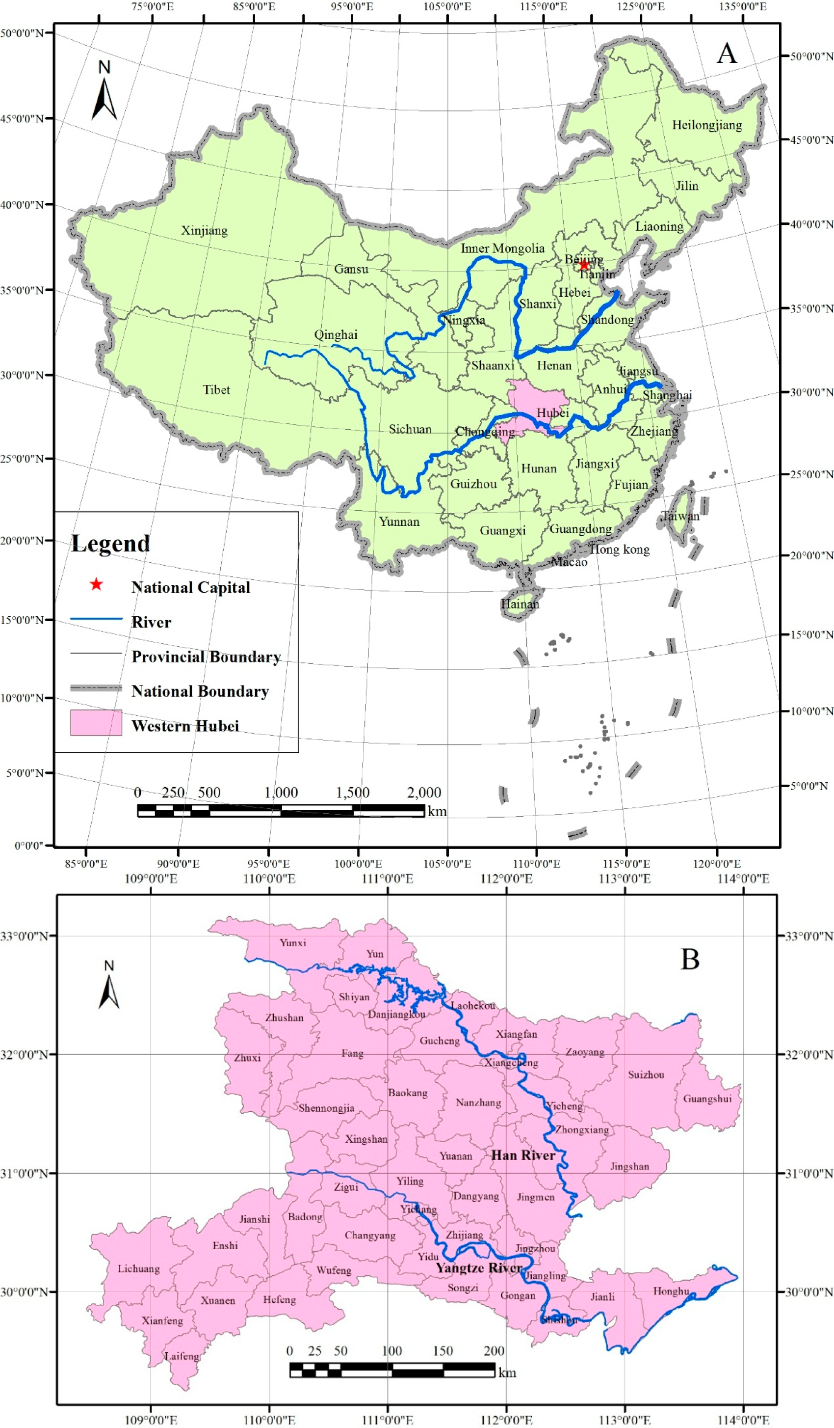
2.1. Characteristics of the Study Area

The study area includes Western Hubei (Figure 1), which encompasses the cities of Xiangyang, Jingzhou, Yichang, Shiyan, Jingmen, Suizhou, Enshi and Shennongjia. The area is 127,847 km² and is located between 108°21′42″–114°33′07″E and 29°1′53″–33°16′47″N in Central China. Western Hubei lies in the marginal zones between the second and third steps of Chinese terrain. The western region is mountainous, the northern region is hilly and the southeastern region features the Jianghan Plain.

Western Hubei is located in a mid-subtropical zone, which is characterised by a typical monsoon climate, four seasons, ample sunshine, and abundant thermal energy resources. Because of the topography and regional disparity, the climate has east-west, north-south and vertical heterogeneity. Sunlight and solar radiation in the east and north are higher than those in the west and south. The annual average temperature is greater than 17 °C in the western valley, less than 15 °C in the alpine areas, and between 15 °C and 17 °C in the remainder of the region. The precipitation is highest in Southwestern Hubei, followed by the Jianghan Plain, Northern Hubei, and Northwestern Hubei. The local rainfall is closely related to the summer monsoon.

Western Hubei is a resource-rich area with various plants. This area has 46,400 km² of forests; the forest coverage is approximately 36.3%. Artificial young and middle-aged forests and natural secondary young and middle-aged forests account for the vast majority of the forests. Western Hubei is one origin of the modern flora in China. Shennongjia, which is considered a national treasure, is a forestry district along the same latitude. The complex ecological and geographical environment has produced diverse vegetation types [22].

2.2. Data Sources and Processing Methods

To conduct this study, the following data (

Table 1. The main data used in this study.

Parameter	Description
Name	Names of the toponyms
Coordinate	X and Y coordinates
Vegetation coverage	NDVI
Topography	Altitude, slope and aspect

) were collected:

• Place name data: All of the toponyms used in this research were collected from the place names database of Hubei Province at the Civil Affairs Department of Hubei. We selected all of the mass self-organisation place names as statistical objects, which included all of the rural villager committee names and urban resident committee names. Because these places were named spontaneously by the community or were named based on geomorphic characteristics, surnames or other factors, smaller places are more likely reflect the local natural landscape than larger places. The place names data can be divided into phytotoponyms and non-phytotoponyms. This is not a common classification method, but that toponyms were classified into these two groups for the purpose of this research, which focuses on phytotoponyms. Phytotoponyms can be further divided into woody plant toponyms and herbaceous plant toponyms. We first chose phytotoponyms according to their literal meanings. We obtained all toponyms that contain the names of plants. However, a few of these toponyms were not phytotoponyms. We excluded the toponyms that share people’s surnames; for example, certain plant names are used as surnames in China, such as poplar (Yang), willow (Liu) and plum (Mei). Additionally, we excluded toponyms named for other factors, such as terrain, or misread names. Note that it was difficult to determine the true motivation behind the origin of certain toponyms in which plant names were recognised. Specifically, we considered that these particular toponyms were phytotoponyms. Finally, we obtained the toponyms that contain the names of plants and were named after plants, phytotoponyms. We randomly selected non-phytotoponyms in every county, and we ensured that equal numbers of phytotoponyms and non-phytotoponyms were selected. We counted the number of phytotoponyms, woody plant toponyms and herbaceous plant toponyms of every county and classified them to 5 levels (

  Table 2. Classification standards for the number of phytotoponyms, altitude, slope and vegetation coverage degree.

  Classification	Number of phytotoponyms	Altitude (m)	Slope (°)	Vegetation coverage degree (%)
  1	0–10	Less than 0	Less than 2	Less than 30
  2	11–20	0–200	2–6	30–45
  3	21–30	200–500	6–15	45–60
  4	31–40	500–1000	15–25	60–75
  5	More than 40	More than 1000	More than 25	More than 75

  ). The classification standards of the number of woody plant toponyms and herbaceous plant toponyms are same with phytotoponyms.
• Coordinate data: To obtain the coordinates for all toponyms, data were selected using Amap coordinates. However, a situation must be considered in which a particular toponym may appear in several counties. The coordinates can help provide the geographical features and NDVI characteristics where the toponyms are located. All of the toponyms were reduced to points in the process of obtaining the geographical features and NDVI characteristics.
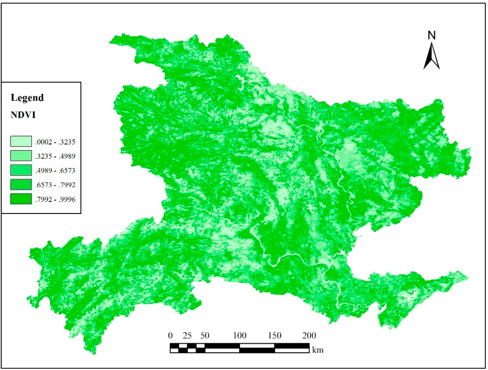
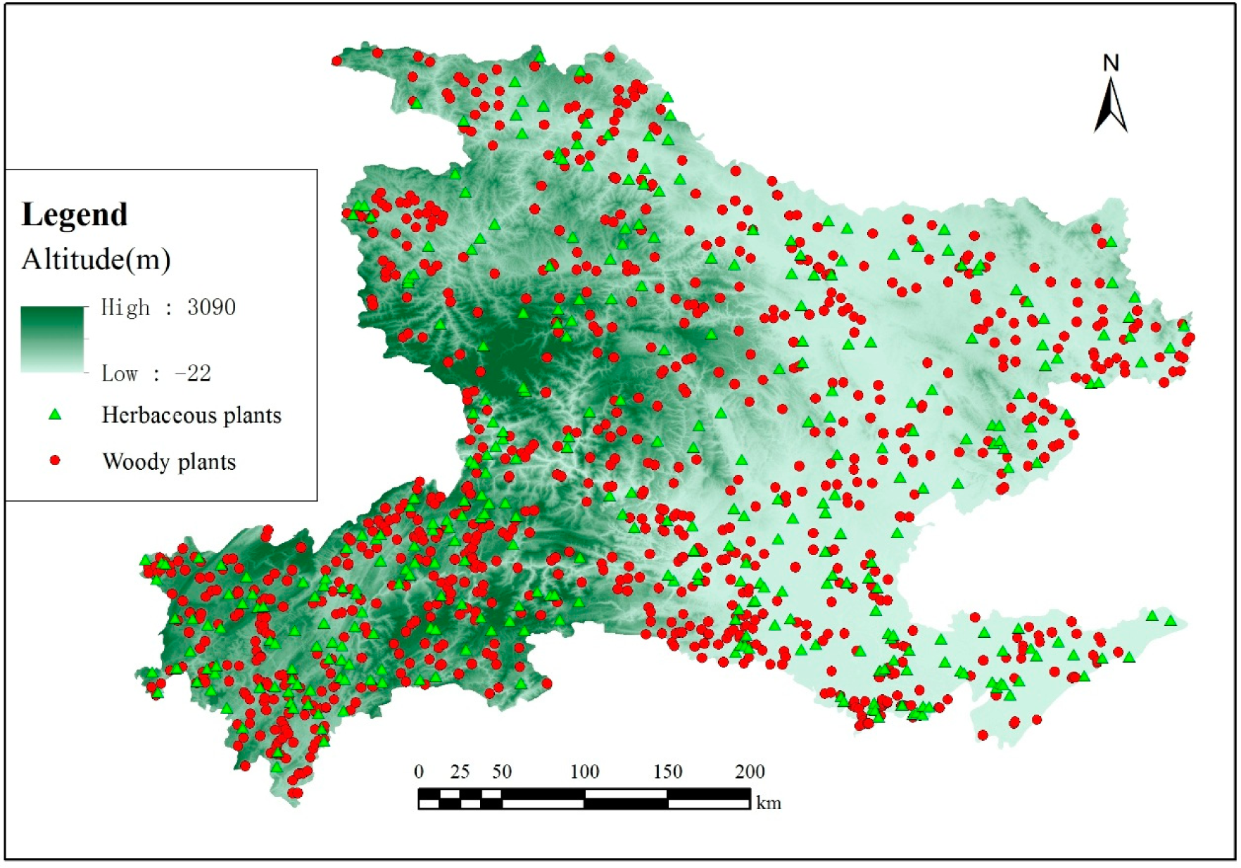
• NDVI: To obtain the vegetation coverage of every location, the NDVI dataset of Western Hubei, with a spatial resolution of 250 m, was downloaded from the Computer Network Information Centre, Chinese Academy of Sciences (Beijing, China), at international scientific data mirror sites. We then used spatial analyst tools to extract values at a point in ArcGIS and obtain the grid value of each location. The vegetation coverage in the study area is presented in Figure 2. There is higher vegetation coverage rate in the western region of the study area than in the middle of the study area. We also obtained the average NDVI of every county. We used f_NDVI to evaluate the vegetation coverage degree of every county [23], the formula of f_NDVI is as follows:

  $$f_{NDVI}=\frac{NDVI-NDV{I}_{\mathit{min}}}{NDV{I}_{\mathit{max}}-NDV{I}_{\mathit{min}}}$$

  (1)

  where NDVI_min and NDVI_max are the minimal and maximum NDVI of all the counties. The f_NDVI value is between 0 and 1. We also classified f_NDVI to 5 levels [24] and the standard presented in Table 2.
• Altitude, slope and aspect data: To obtain the altitude, slope and aspect data of each location, digital elevation models (DEMs), slopes and aspects of Western Hubei, with a spatial resolution of 90 m, were downloaded from the Computer Network Information Centre, Chinese Academy of Sciences, China, at international scientific data mirror sites. We obtained the grid value of each location using the same method described for the NDVI data. We also obtained the average altitude and slope of every county and classified them to five levels according to the standards [25,26]. The specific standards are presented in Table 2.

2.3. Statistical Analysis

The linguistic features associated with the phytotoponyms are shown using statistical tables. Box-plot graphs were used to present the topography and NDVI dataset characteristics. Because the topography and NDVI data were non-normally distributed, we performed comparison tests between phytotoponyms and non-phytotoponyms, woody plant toponyms and herbaceous plants toponyms using the non-parametric two-sample Wilcoxon rank sum test with SPSS software. The Wilcoxon rank sum test is solely based on the order of the observations of the two samples. First, all observations are arranged into a single ranked series. That is, all of the observations are ranked regardless of which sample they belong to. Second, the ranks for the observations from sample 1 are added together. When groups have equal rankings, the rank equal to the midpoint of the group was taken. The sum of ranks in sample 2 is now determinate because the sum of all of the ranks equals N × (N + 1)/2, where N is the total number of observations. Then, U is given by [27]:

$${\mathrm{U}}_1=n_1{n}_2+\frac{n_1\left(n_1+1\right)}{2}-R_1$$

(2)

$${\mathrm{U}}_2=n_1{n}_2+\frac{n_2\left(n_2+1\right)}{2}-R_2$$

(3)

where n₁ and n₂ are the sample sizes for samples 1 and 2, respectively, and R₁ and R₂ are the sums of the ranks in samples 1 and 2, respectively. The smaller value of U₁ or U₂ is used when consulting significance tables [28]. The null hypothesis of the Wilcoxon rank sum test is that there is no difference between the responses of the two samples. If the probability of the null hypothesis is very small (e.g., p < 0.05 or 0.01), we must reject the null hypothesis, indicating a difference between the two samples.

2.4. Information Entropy Calculation

In our study, we used information entropy to evaluate the correlation between the number of phytotoponyms and altitude, slope and vegetation coverage degree. The information entropy calculation formula is as follows:

$$\mathrm{H}\left(\mathrm{X}\right)=\mathrm{E}\left[\mathrm{I}\left(\mathrm{X}\right)\right]=\mathrm{E}[-\ln (P\left(X\right))]$$

(4)

where H(X) is the information entropy, X is the discrete random variable; P(X) is the probability mass function. And E is the expected value operator, I is the information content of X [29]. When taken from a finite sample, the information entropy can explicitly be written as follows:

$$\mathrm{H}\left(\mathrm{X}\right)={\displaystyle \sum }_{i}P\left(x_i\right)I\left(x_i\right)=-{\displaystyle \sum }_{i}P(x_i){\log }_{b}P(x_i)$$

(5)

where b is the base of the logarithm used. Common values of b are 2, Euler’s number e, and 10, and the unit of entropy is Shannon for b = 2, nat for b = e, and Hartley for b = 10. Joint entropy is a measure of the uncertainty associates with a set of variables. The joint entropy of two variables X and Y is defined as Equation (6):

$$\mathrm{H}\left(\mathrm{X},\mathrm{Y}\right)=-{\displaystyle \sum }_x{\displaystyle \sum }_{y}P(x,y){\log }_2[P(x,y)]$$

(6)

where x and y are particular values of X and Y, respectively, P(x, y) is the joint probability of these values occurring together. The joint entropy of two variables is less than or equal to the sum of the individual entropies of the two variables:

$$\mathrm{H}\left(\mathrm{X},\mathrm{Y}\right)\le \mathrm{H}\left(\mathrm{X}\right)+\mathrm{H}(\mathrm{Y})$$

(7)

This inequality is equality if and only if X and Y are statistically independent. So H(X, Y)/H(X) + H(Y) can reflect the correlation between X and Y. We often used K to describe the correlation degree between X and Y, the formula of K is as follows [30]:

$$\mathrm{K}=1-\frac{H(X,Y)}{H\left(X\right)+H(Y)}$$

(8)

The K value is between 0 and 1 because H(X,Y) ≤ H(X)+H(Y). K is equal to zero if X and Y are statically independent. The greater value of K is, the stronger correlation between X and Y.

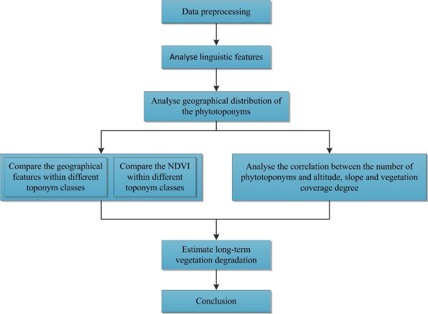
2.5. Technology Flow Chart

The main workflow of this study is presented in Figure 3. First, we chose phytotoponyms and analysed the linguistic features of the phytotoponyms. Then, we obtained the coordinates of the phytotoponyms using the Amap coordinates picker and drew the thematic map of the geographic distribution of the phytotoponyms. We then extracted the grid values of each location using ArcGIS. Additionally, we performed this same protocol using non-phytotoponyms.

Subsequently, we analysed the differences between phytotoponyms and non-phytotoponyms and between woody plant toponyms and herbaceous plants toponyms using the Wilcoxon rank sum test. Then, we calculated the correlation between the number of phytotoponyms and altitude, slope and vegetation coverage degree using information entropy theory. Finally, we estimated long-term vegetation degradation and drew the thematic map of the geographical distribution of the vegetation degradation toponyms.

3. Results and Discussion

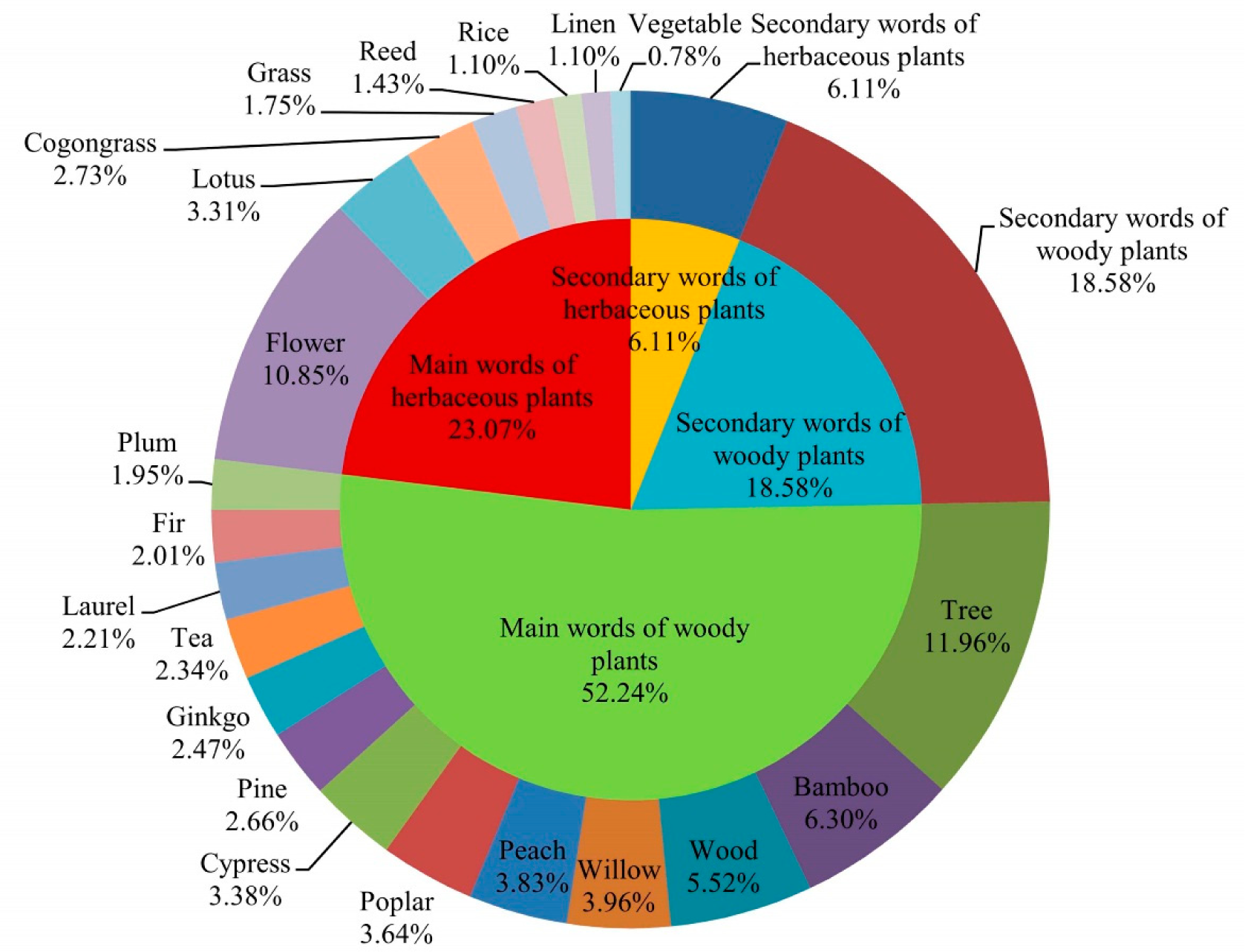
3.1. Linguistic Features of the Phytotoponyms

In the study area, 15,465 mass self-organisation place names were recorded; 1259 (8.14%) were phytotoponyms, including 898 (71.3%) woody plant toponyms and 361 (28.7%) herbaceous plant toponyms. The phytotoponyms and a subset of the non-phytotoponyms (1250) were assigned coordinates and geo-referenced.

The plant names recognised in the phytotoponyms of Western Hubei (

Table 3. Linguistic features of the phytotoponyms in western Hubei.

Class	Main words	Frequency of occurrence	Ratio of occurrence (%)	Secondary words	Frequency of occurrence	Ratio of occurrence (%)
Woody plants	Tree	184	11.96	Chestnut	286	18.58
	Bamboo	97	6.30	Paulownia
	Wood	85	5.52	Pear
	Willow	61	3.96	Vitex
	Peach	59	3.83	Catalpa
	Poplar	56	3.64	Walnut
	Cypress	52	3.38	Wingceltis
	Pine	41	2.66	Mulberry
	Ginkgo	38	2.47	Robinia
	Tea	36	2.34	Birch
	Laurel	34	2.21	Tangerine
	Fir	31	2.01	Maple
	Plum	30	1.95	Oak, etc.
Herbaceous plants	Flower	167	10.85	Orchid	94	6.11
	Lotus	51	3.31	Rattan
	Cogongrass	42	2.73	Artemisia
	Grass	27	1.75	Smartweed
	Reed	22	1.43	Ginger
	Rice	17	1.10	Medicine
	Linen	17	1.10	Chrysanthemum
	Vegetable	12	0.78	Wheat, etc.
Total		1159	75.31		380	24.69

) are listed according to their plant category and ratio of occurrence (frequency of occurrence of a particular plant/total frequency of occurrence for all plants × 100%). Figure 4 further shows the ratio of occurrence for the different plant categories. Plant names appeared 1539 times in 1259 phytotoponyms (in some case, two or more plant names were recognised in one phytotoponym, and thus, the total frequency of the occurrence for all plants is greater than the number of phytotoponyms). Certain words that did not represent unique plants were common, such as “tree”, “wood” and “flower”. These words are simple and often used in daily life, and thus, they are likely to appear in place names. Some common plant species, such as “bamboo”, “willow”, “peach” and “lotus”, also appeared frequently. These plant species are closely related to human life and provide a source of food, building material and various raw materials. In addition, most of these species are associated with positive morals in Chinese culture and literature.

We further statistically analysed the plant names (

Table 4. Linguistic features of the phytotoponyms in eight cities.

City	Number of phytotoponyms	Proportion of phytotoponyms relative to the total toponyms (%)	Plant in the phytotoponym			Characteristic plant of a city
			No.	Unique plants	Frequency of occurrence
Shiyan	179	9.54	1	Bamboo	13	Tea Papaya Rice
			2	Willow	9
			3	Cypress	9
			4	Lotus	7
			5	Ginkgo	6
			6	Tea	5
			7	Papaya	4
			8	Palm	3
			9	Rice	2
Enshi	420	16.03	1	Bamboo	31	Tea Paulownia Lacquer
			2	Ginkgo	20
			3	Tea	18
			4	Cypress	16
			5	Plum	12
			6	Paulownia	10
			7	Chestnut	9
			8	Lacquer	5
Xiangyang	124	5.71	1	Bamboo	14	Tea Willow
			2	Lotus	9
			3	Peach	7
			4	Cypress	6
			5	Willow	6
			6	Pine	5
			7	Tea	4
			8	Plum	3
Yichang	154	11.16	1	Bamboo	12	Tea Tangerine Walnut
			2	Willow	11
			3	Plum	6
			4	Pine	8
			5	Laurel	7
			6	Poplar	6
			7	Nanmu	5
			8	Tangerine	4
			9	Tea	3
			10	Walnut	1
Suizhou	69	8.27	1	Peach	4	Ginkgo
			2	Cypress	4
			3	Willow	4
			4	Plum	3
			5	Ginkgo	3
			6	Wingceltis	3
			7	Saponin	2
Jingmen	87	7.79	1	Bamboo	8
			2	Willow	5
			3	Poplar	4
			4	Jujube	4
			5	Lotus	4
			6	Chestnut	3
			7	Catalpa	3
			8	Vitex	2
Jingzhou	211	8.16	1	Poplar	16	Lotus
			2	Bamboo	15
			3	Lotus	11
			4	Reed	9
			5	Willow	8
			6	Fir	6
			7	Laurel	6
			8	Oak	3
			9	Plum	2
			10	Water chestnut	2
Shennongjia	15	20.55	1	Peach	2
			2	Lotus	2
			3	Cypress	2

) and presented the three plant names that most frequently occur (Figure 5) in the phytotoponyms of each city. To reflect the characteristic plants of a city, we excluded words that do not represent a unique plant. Some common plant species appeared at a high frequency in most cities. For example, “bamboo” was the most frequent plant in cities, including in Shiyan, Enshi, Xiangyang, Yichang and Jingmen. Occasionally, plant names in phytotoponyms can reflect the characteristic plants of a particular area. This is especially true in cities that have large number of phytotoponyms and a high proportion of phytotoponyms. For example, “papaya” only appeared five times in the phytotoponyms in Western Hubei, four of which were in Shiyan, a papaya-rich area. Similar cases were observed for “Paulownia” and “lacquer” in Enshi. Two cities, Jingmen and Shennongjia, do not have the characteristic plants related to the plant names found in the phytotoponyms. Because Jingmen does not have characteristic plants and Shennongjia has few phytotoponyms, it is difficult to reflect the characteristic plants.

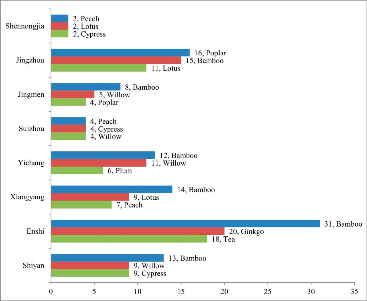
3.2. Geographical Distribution of the Phytotoponyms

The distributions of the different phytotoponym classes throughout the entire study area are shown in Figure 6. Phytotoponyms were more frequent in the mountainous region of Southwestern Hubei and the Jianghan Plain and less frequent in hilly Northern and Central Hubei. There was no obvious difference between the distributions of woody plant toponyms and herbaceous plant toponyms. Note that Figure 6 only shows that the absolute number of phytotoponyms has a close relationship with the total number of toponyms of an area. For example, Shennongjia only has 15 phytotoponyms but has a high proportion (20.55%) of phytotoponyms relative to the total toponyms.

3.3. The Relationship Between Topography and Phytotoponyms

Figure 7 shows the topographic features of the different toponym classes. The different toponym classes display similar distributions regarding the aspect, showing no predominant orientation. The slopes where woody plant toponyms are located differ significantly from the herbaceous plant toponyms. The average slope where woody plant toponyms are located is steeper than that of the herbaceous plant toponyms. This may indicate that woody plants can adapt to a steeper slope than herbaceous plants and because steeper slopes are less suitable for agriculture, they remained forested, whereas less steep slopes were cultivated. There was no significant difference in the slopes of the phytotoponyms and non-phytotoponyms; the slope distributions were also similar. Phytotoponyms were located at significantly higher altitudes, whereas non-phytotoponyms tended to be at lower altitudes. The altitudes where woody plant toponyms are located were not significantly different from those of herbaceous plant toponyms.

The Wilcoxon rank sum test results are presented in

Table 5. Wilcoxon rank sum test results that compare topographies (altitude, slope and aspect) of phytotoponyms and non-phytotoponyms.

	Altitude	Slope	Aspect
Mann-Whitney U	741,693.500	752,102	783,214
Wilcoxon W	1,523,568.500	1,533,977	1,565,089
Z	−2.490	−1.927	−0.202
Asymptotic significance (double-sided)	0.013	0.054	0.840

Grouping variable: whether the toponym is a phytotoponym.

and

Table 6. Wilcoxon rank sum test results comparing the topographies (altitude, slope and aspect) of woody plants and herbaceous plants.

	Altitude	Slope	Aspect
Mann-Whitney U	154,768.500	148,425.500	157,966.000
Wilcoxon W	220,109.500	213,766.500	561,617.000
Z	−1.255	−2.353	−0.707
Asymptotic significance (double-sided)	0.210	0.019	0.480

Grouping variable: whether the phytotoponym is a woody plant.

. In Table 5, the asymptotic significance of the Wilcoxon rank sum test that compares altitude of phytotoponyms and non-phytotoponyms is less than 0.05, which indicates that the altitudes where phytotoponyms are located differ significantly from those of non-phytotoponyms. In Table 6, the asymptotic significance of the Wilcoxon rank sum test that compares the slope of woody plant toponyms and herbaceous plant toponyms is less than 0.05, which indicates that the slopes where woody plant toponyms are located differ significantly from the slopes for herbaceous plant toponyms.

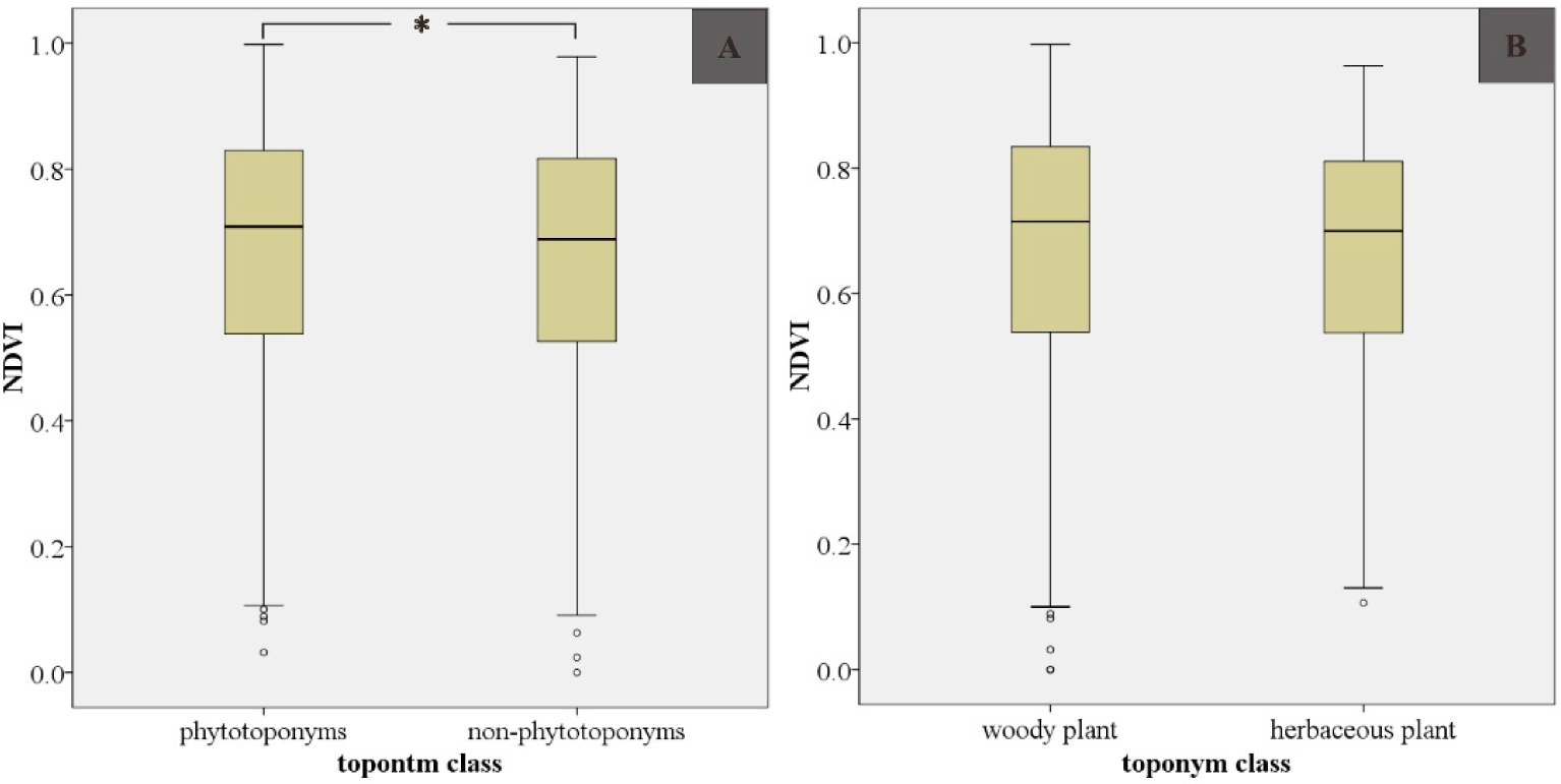
3.4. The Relationship Between NDVI and Phytotoponyms

The NDVI values of the different toponym classes are shown in Figure 8. The NDVI of the phytotoponym areas differed significantly from that of the non-phytotoponym areas. The average NDVI of phytotoponym areas was higher than that of the non-phytotoponym areas. Therefore, the places where phytotoponyms are located showed higher vegetation coverage rate than non-phytotoponym areas. No significant differences regarding the NDVI were detected between woody plant toponyms and herbaceous plant toponyms. The Wilcoxon rank sum test results are given in

Table 7. Wilcoxon rank sum test results comparing the vegetation coverage (NDVI) of phytotoponyms and non- phytotoponyms.

	NDVI
Mann-Whitney U	751,198.500
Wilcoxon W	1,533,073.500
Z	−1.966
Asymptotic significance (double-sided)	0.049

Grouping variable: whether the toponym is a phytotoponym.

and

Table 8. Wilcoxon rank sum test results that compares vegetation coverage (NDVI) of woody plants and herbaceous plants.

	NDVI
Mann-Whitney U	157,480.000
Wilcoxon W	222,821.000
Z	−0.790
Asymptotic significance (double-sided)	0.430

Grouping variable: whether the toponym is a woody plant.

. A significant difference was observed between phytotoponyms and non-phytotoponyms based on the NDVI, whereas the difference between woody plant toponyms and herbaceous plant toponyms was not significant.

3.5. Correlation Analysis based on Information Entropy Theory

The joint distribution probability matrix between the number of phytotoponyms and altitude, slope and vegetation coverage degree (f_NDVI) are given in

Table 9. Joint distribution probability matrix between the number of phytotoponyms and altitude.

Altitude (m)	Number of phytotoponyms					P(yi)
	Less than 10	10–20	20–30	30–40	More than 40
Less than 0	0	0	0	0	0	0
0–200	4/46	6/46	5/46	3/46	2/46	20/46
200–500	1/46	3/46	1/46	0	0	5/46
500–1000	0	3/46	6/46	1/46	1/46	11/46
More than 1000	0	3/46	0	2/46	5/46	10/46
P(xi)	5/46	15/46	12/46	6/46	8/46	1

–

Table 11. Joint distribution probability matrix between the number of phytotoponyms and vegetation coverage degree.

Vegetation coverage degree (%)	Number of phytotoponyms					P(yi)
	Less than 10	10–20	20–30	30–40	More than 40
Less than 30	1/46	2/46	0	0	0	3/46
30–45	3/46	1/46	2/46	0	0	6/46
45–60	0	6/46	2/46	1/46	1/46	10/46
60–75	1/46	2/46	3/46	2/46	4/46	12/46
More than 75	0	4/46	5/46	3/46	3/46	15/46
P(xi)	5/46	15/46	12/46	6/46	8/46	1

.

The probabilistic distribution of the number of phytotoponyms is evenly. 15 counties have 10–20 phytotoponyms, only five counties less than 10 phytotoponyms. There are 20 counties’ average altitude in the 0–200 m and all counties’ average altitude above sea level. There are 19 counties’ average slopes in the 15–25° but only one’s more than 25°. The probabilistic distribution of vegetation coverage degree is evenly. Information entropy of the number of phytotoponyms, altitude, slope and vegetation coverage degree was calculated by Equation (5). The results presented in

Table 12. Information entropy of the number of phytotoponyms, altitude, slope and vegetation coverage degree.

	Number of phytotoponyms	Altitude	Slope	Vegetation coverage degree
Information entropy	2.203	1.843	1.999	2.152

. The information entropy of the number of phytotoponyms is the highest and the information entropy of altitude is the lowest. That means the distribution of the number of phytotoponyms is more balanced and the distribution of altitude is more concentrated.

Joint entropy of the number of phytotoponyms and altitude, slope and vegetation coverage degree could be calculated by Equation (6). K value could be calculated by Equation (8) further. We also calculated the K value using the number of woody plant toponyms and herbaceous plant toponyms substitute for the number of phytotoponyms. The results presented in

Table 13. K value of the number of phytotoponyms, woody plant toponyms with herbaceous plant toponyms and altitude, slope as well as vegetation coverage degree.

	Altitude	Slope	Vegetation coverage degree
Number of phytotoponyms	0.0916	0.0786	0.0897
Number of woody plant toponyms	0.0703	0.0550	0.0651
Number of herbaceous plant toponyms	0.0455	0.0370	0.0295

.

The K value could evaluate the correlation between two factors. The greater the value of K is, the stronger correlation between factor A and B. The number of phytotoponyms has stronger correlation with altitude, slope and vegetation coverage degree than the number of woody plant toponyms and herbaceous plant toponyms. Altitude has a stronger correlation with the number of phytotoponyms, woody plant toponyms and herbaceous plant toponyms than slope and vegetation coverage degree. The K value of altitude and the number of phytotoponyms is the highest, closely followed by vegetation coverage degree and the number of phytotoponyms. So the number of phytotoponyms has correlation with altitude and vegetation coverage degree. This result is similar with the result of Wilcoxon rank sum test that phytotoponyms and non-phytotoponyms have significant differences on altitude and NDVI.

3.6. Estimating Long-term Vegetation Degradation Using Phytotoponyms

The motive for naming a place using a phytotoponym is that the given area includes a specific plant. The Wilcoxon rank sum test results show that the average NDVI values where phytotoponyms are located are higher than those in non-phytotoponym areas. The number of phytotoponyms has correlation with vegetation coverage degree. Informed research has shown that toponyms often survive changes in the local landscape [4]. Thus, we assume that the places where phytotoponyms are located have very high vegetation coverage rate. Furthermore, if the area only has a low NDVI, then vegetation degradation has occurred in this area. Considering that Western Hubei has high vegetation coverage rate, we believe that a low NDVI indicates that no vegetation coverage is equal to the smallest decile. Places having phytotoponyms and an NDVI less than the smallest decile are identified (Figure 9), and the names of these places are referred to as vegetation degradation toponyms.

Table 14. The vegetation degradation ratio of every county.

County	Vegetation degradation ratio (%)	Number of vegetation degradation toponyms	Number of phytotoponyms	Number of toponyms	The proportion of phytotoponyms (%)
Jiangling	40.00	4	10	222	4.5
Xiangcheng district	40.00	4	10	172	5.81
Gucheng	30.77	4	13	290	4.48
Yidu	26.67	4	15	145	10.34
Yicheng	25.00	2	8	206	3.88
Changyang	21.74	5	23	159	14.47
Xuanen	20.00	9	45	284	15.49
Enshi	17.07	7	41	206	19.9
Hefeng	16.13	5	31	201	14.93
Nanzhang	15.00	3	20	304	6.58
Gongan	15.00	3	20	374	5.35
Jingzhou municipal district	15.00	3	20	321	6.23
Danjiangkou	14.81	4	27	246	10.98
Laohekou	12.50	1	8	258	3.1
Zigui	12.50	2	16	193	8.29
Zhijiang	12.50	2	16	214	7.48
Yiling district	11.76	2	17	223	7.62
Jianshi	11.59	8	69	393	17.56
Xianfeng	11.54	6	52	289	17.99
Yun	10.00	3	30	350	8.57
Xiangfan municipal district	10.00	2	20	829	2.41
Jingshan	9.09	3	33	430	7.67
Dangyang	8.33	1	12	185	6.49
Yunxi	8.00	2	25	341	7.33
Songzi	7.84	4	51	473	10.78
Fang	7.41	2	27	288	9.38
Jingmen municipal district	6.90	2	29	577	5.03
Lichuan	5.88	5	85	585	14.53
Laifeng	5.71	2	35	196	17.86
Yichang municipal district	5.00	1	20	510	3.92
Badong	5.00	3	60	491	12.22
Baokang	4.55	1	22	279	7.89
Zaoyang	4.17	1	24	566	4.24
Zhongxiang	4.00	1	25	546	4.58
Suizhou	2.94	1	34	541	6.28
Guangshui	2.86	1	35	401	8.73
Shishou	1.82	1	55	802	6.86
Honghu	0	0	29	494	5.87
Zhuxi	0	0	36	292	12.33
Shiyan municipal district	0	0	11	168	6.55
Zhushan	0	0	23	264	8.71
Shennongjia	0	0	15	73	20.55
Xingshan	0	0	12	96	12.5
Yuanan	0	0	5	46	10.87
Wufeng	0	0	19	109	17.43
Jianli	0	0	26	833	3.12
Total	——	114	1259	15465	——
Average	9.05	2.48	27	336	8.04

shows the vegetation degradation ratio of every county (number of vegetation degradation toponyms/number of phytotoponyms × 100%).

The geographical distribution of the vegetation degradation toponyms was more dispersed overall. Only small areas of concentrated toponyms were found in the mountainous region of Southwestern Hubei. There are no vegetation degradation toponyms in the mountainous region of the west, including Shennongjia, Zhushan and Zhuxi. Jiangling, Xiangcheng District, and Gucheng and Yicheng counties have high vegetation degradation ratios but low proportions of phytotoponyms. Yidu, Changyang, Xuanen, Enshi and Hefeng counties showed a high vegetation degradation ratio and high proportion of phytotoponyms. The counties with high vegetation degradation ratios are more likely to experience vegetation degradation.

There are undoubtedly many shortcomings in this approach for calculating the vegetation degradation of study area. Not all of the places where phytotoponyms are located have high vegetation coverage rate. Additionally, the places where phytotoponyms are located cannot replace the entire study area, and the standards used to identify vegetation degradation are not rigorous. However, as a new method for calculating vegetation degradation based on toponyms, the results are worth considering and serve as a reference. Because toponyms were generated long time ago, this approach is conducive for studying long-term vegetation degradation.

4. Conclusions

In this paper, we performed a series of studies on phytotoponyms in Western Hubei, China, including semantic analysis, geographical feature and vegetation coverage analysis, correlation analysis between the number of phytotoponyms and altitude, slope as well as vegetation coverage degree and coarse vegetation degradation estimations. This research fully utilized the information contained in the phytotoponyms using geo-referencing.

The approach used in this paper has certain methodological limitations. First, although the place name data were obtained from the toponyms database of the Hubei Provincial Civil Affairs Department, it is still difficult to rule out a number of factors, including dialects and homophones. It is also difficult to determine the true motivation behind the use several phytotoponyms that may not stem from plants but rather are associated with a person, object or event that is only indirectly connected to the plant [18]. Second, each place represented by a toponym has a different area and shape; however, all places were reduced to points. The descriptions of the geographical features and NDVI values also lack the precision needed for modelling grid points of the 90 m × 90 m digital elevation model and the 250 m × 250 m normalised difference vegetation index. But there is no alternative method; this process is the only method of obtaining the vegetation coverage and geographical features for a small area like the rural villager committee and urban resident committee. We cannot obtain detailed boundaries for such a small area because of the administrative area change and parts of boundary are not clear itself. In addition, such an approach may appear unreasonable, but with a large number of toponyms, this approach is statistically reliable.

Nevertheless, some valuable conclusions were obtained. We obtained the basic information on phytotoponyms in Western Hubei, and 1259 instances of phytotoponyms were recognised; 898 (71.3%) were woody plant toponyms, and 361 (28.7%) were herbaceous plant toponyms. Plant names appeared 1539 times in 1259 phytotoponyms. Certain words such as “tree”, “wood” and “flower” were common, and “bamboo”, “willow”, “peach” and “lotus” also appeared frequently. Phytotoponyms are common products of the natural landscape and social customs, and these names are influenced by vegetation coverage. However, the importance of a plant in people’s life, the cultural implication of this plant, and even the social development level will affect the phytotoponym. Thus, the phytotoponym can reflect the characteristic plants, the vegetation coverage of the historical period and the cultural heritage of a particular place.

Phytotoponyms were more frequent in the mountainous region of Southwestern Hubei and the Jianghan Plain and were less frequent in hilly Northern and Central Hubei. There was no obvious difference in the distribution of woody plant toponyms and herbaceous plant toponyms.

The statistical results indicated that the places where phytotoponyms are located have higher vegetation coverage rate and higher altitudes than non-phytotoponym areas; woody plants can adapt to steeper slopes than herbaceous plants. The information entropy calculation results indicated that the number of phytotoponyms and altitude and vegetation coverage degree have correlations. These results are similar with the results of the Wilcoxon rank sum test.

The geographical distribution of the vegetation degradation toponyms was more dispersed overall. Only small areas of concentrated toponyms were found in the mountainous region of Southwestern Hubei. Phytotoponyms may be a useful tool when combined with other techniques for studying long-term vegetation degradation.

References

1. Encyclopedia of China: Geography Toponym; Encyclopedia of China Publishing House: Beijing, China, 1992.
2. Kadmon, N. Toponymy: The Lore, Laws, and Language of Geographical Names; Vantage Press: New York, NY, USA, 2000. [Google Scholar]
3. Pu, S.X. Theory and Application of Geographic Names Information System—Digital Names; Xinhua Publishing House: Beijing, China, 2000. [Google Scholar]
4. Conedera, M.; Vassere, S.; Neff, C.; Meurer, M.; Krebs, P. Using toponymy to reconstruct past land use: a case study of ‘brüsáda’ (burn) in southern Switzerland. J. Hist. Geogr. 2007, 33, 729–748. [Google Scholar]
5. Henshaw, A. Pausing along the journey: Learning landscapes, environmental change, and toponymy amongst the Sikusilarmiut. Arct. Anthropol. 2006, 43, 52–66. [Google Scholar]
6. Ford, R.E.; Toponymic, Generics. Environment, and Culture History in Pre-Independence Belize*. Names 1991, 39, 1–26. [Google Scholar]
7. Tucci, M.; Ronza, R.W.; Giordano, A. Fragments from many pasts: Layering the toponymic tapestry of Milan. J. Hist. Geogr. 2011, 37, 370–384. [Google Scholar]
8. Alderman, D.H. Street names and the scaling of memory: The politics of commemorating Martin Luther King, Jr within the African American community. Area 2003, 35, 163–173. [Google Scholar]
9. Horsman, S. The politics of toponyms in the Pamir Mountains. Area 2006, 38, 279–291. [Google Scholar]
10. Yeoh, B.S. Street-naming and nation-building: Toponymic inscriptions of nationhood in Singapore. Area 1996, 28, 298–307. [Google Scholar]
11. Wang, F.; Zhang, L.; Zhang, G.; Zhang, H. Mapping and spatial analysis of multiethnic toponyms in Yunnan, China. Cartogr. Geogr. Inf. Sci. 2014, 41, 86–99. [Google Scholar]
12. Wang, F.; Wang, G.; Hartmann, J.; Luo, W. Sinification of Zhuang place names in Guangxi, China: A GIS-based spatial analysis approach. Trans. Inst. Br. Geogr. 2012, 37, 317–333. [Google Scholar]
13. Guan, Y.B. Placename and Geographical Distribution of Nationality. J. Guizhou Norm. Univ. (Soc. Sci.) 2007, 3, 13–19. [Google Scholar]
14. Seidl, N.P. Significance of Toponyms, with Emphasis on Field Names, for Studying Cultural Landscape. Acta Geogr. Slov. 2008, 48, 33–56. [Google Scholar]
15. Wang, B.; Situ, S. Analysis of spatial characteristics of place names landscape based on GIS technology in Guangdong Province. Geogr. Res. 2007, 2, 238–148. [Google Scholar]
16. Li, J.H.; Mi, B.W.; Feng, C.Y.; Yang, X.M. An analysis on toponym cultural landscape based on GIS application in Zhongwei county, Ningxia municipality. Hum. Geogr. 2011, 1, 100–104. [Google Scholar]
17. Wang, B.; Yue, H. EOF Model Analysis of Place Names Landscape in Guangdong Province on GIS. Geogr. Sci. 2007, 2, 281–288. [Google Scholar]
18. Čargonja, H.; Đaković, B.; Alegro, A. Plants and Geographical Names in Croatia. Coll. Anthr. 2008, 32, 927–943. [Google Scholar]
19. Guarino, R. A survey of the botanical place names of the Iglesiente Area (south west Sardinia). Bot. Lith. 2007, 13, 139–157. [Google Scholar]
20. Shannon, C.E. A Mathematical Theory of Communication. Bell Syst. Tech. J. 1948, 27, 379–423. [Google Scholar]
21. Chen, X.X.; Hu, T.; Ren, F.; Chen, D.; Li, L.; Gao, N. Landscape Analysis of Geographical Names in Hubei Province, China. Entropy 2014, 16, 6313–6337. [Google Scholar]
22. Hubei Provincial Development Strategic Planning Office. The charm of Western Hubei (in Chinese). Available online: http://www.exiquan.com.cn/ZX/mlexiquan.aspx accessed on 28 June 2014.
23. Niu, B.R.; Liu, J.R.; Wang, Z.W. Remote Sensing Information Extraction Based on Vegetation Fraction in Drought and Half-Drought Area. Geomat. Inf. Sci. Wuhan Univ. 2005, 30, 27–30. [Google Scholar]
24. Shi, T.T.; Chen, Z.H.; Wang, N.T.; Jin, X.W. Spatial correlation analysis on soil organic carbon and the influencing factors in the Xiangxi River Basin. Carsologica Sin. 2005, 30, 422–431. [Google Scholar]
25. Li, B.; Pan, B.; Han, J. Basic terrestrial geomorphological types in China and their circumscriptions. Quat. Sci. 2008, 28, 535–543. [Google Scholar]
26. The Land Use Updating Investigation Technical Regulations; Ministry of Land and Resources of the People’s Republic of China: Beijing, China, 2003.
27. Zar, J.H. Biostatistical Analysis; Pearson Education India: Chennai, India, 1999. [Google Scholar]
28. Lehmann, E.L.; D’Abrera, H.J. Nonparametrics: Statistical Methods Based on Ranks; Springer: New York, NY, USA, 2006; p. 464. [Google Scholar]
29. Borda, M. Fundamentals in Information Theory and Coding; Springer: New York, NY, USA, 2011; Volume 6. [Google Scholar]
30. Meyer, W.B.; Turner, B.L., II. Changes in Land Use and Land Cover: A Global Perspective; Cambridge University Press: Cambridge, UK, 1994; Volume 4. [Google Scholar]
Figure 1. Study area. (A) Map of China; (B) Map of western Hubei.
Entropy 17 00984f1
Figure 2. Vegetation coverage in the study area.
Entropy 17 00984f2
Figure 3. Methodology flow chart.
Entropy 17 00984f3
Figure 4. The ratio of occurrence for the different plant categories.
Entropy 17 00984f4
Figure 5. The three plant names that most frequently occur in each city.
Entropy 17 00984f5
Figure 6. Geographical distribution of the phytotoponyms in the study area.
Entropy 17 00984f6
Figure 7. Comparison of topographic features between phytotoponyms and non-phytotoponyms (A, aspect; C, slope; E, altitude) and between woody plants and herbaceous plants (B, aspect; D, slope; F, altitude) (*p < 0.05).
Entropy 17 00984f7
Figure 8. Comparison of vegetation coverage (NDVI) between phytotoponyms and non-phytotoponyms (A) and between woody plants and herbaceous plants (B) (* p < 0.05).
Entropy 17 00984f8
Figure 9. Geographical distribution of the vegetation degradation toponyms.
Entropy 17 00984f9