Feeding Back the Output or Sharing the State: Which Is Better for the State-Dependent Wiretap Channel?

Abstract

In this paper, the general wiretap channel with channel state information (CSI) at the transmitter and noiseless feedback is investigated, where the feedback is from the legitimate receiver to the transmitter, and the CSI is available at the transmitter in a causal or noncausal manner. The capacity-equivocation regions are determined for this model in both causal and noncausal cases, and the results are further explained via Gaussian and binary examples. For the Gaussian model, we find that in some particular cases, the noiseless feedback performs better than Chia and El Gamal’s CSI sharing scheme, i.e., the secrecy capacity of this feedback scheme is larger than that of the CSI sharing scheme. For the degraded binary model, we find that the noiseless feedback performs no better than Chia and El Gamal’s CSI sharing scheme. However, if the cross-over probability of the wiretap channel is large enough, we show that the two schemes perform the same.

1. Introduction

It is known to all that the capacity of a point-to-point discrete memoryless channel (DMC) cannot be increased by using noiseless feedback. However, does the feedback (from the legitimate receiver to the transmitter) enhance the security of the wiretap channel? Ahlswede and Cai [1] and Dai et al. [2] studied this problem. Specifically, Ahlswede and Cai [1] showed that the secrecy capacity $C_{sf}$ of the degraded wiretap channel with noiseless feedback is given by:

$$\begin{array}{ccc}& & C_{sf}=\underset{p\left(x\right)}{max}min\{I(X;Y),I(X;Y)-I(X;Z)+H\left(Y\right|X,Z)\},\hfill \end{array}$$

(1)

where X, Y and Z are for the transmitter, legitimate receiver and wiretapper, respectively, and $X\to Y\to Z$ forms a Markov chain. Recall that the secrecy capacity $C_s$ of the degraded wiretap channel is determined by Wyner [3], and it is given by:

$$\begin{array}{ccc}& & C_s=\underset{p\left(x\right)}{max}min\{I(X;Y),I(X;Y)-I(X;Z)\}.\hfill \end{array}$$

(2)

From (1) and (2), it is easy to see that the noiseless feedback increases the secrecy capacity of the wiretap channel. Based on the work of [1], Dai et al. [2] studied a special wiretap channel with feedback ($Y\to X\to Z$) and showed that the secrecy capacity of this model is larger than that of the model without feedback, i.e., the noiseless feedback helps to enhance the security of the special wiretap channel $Y\to X\to Z$. Here, note that in [1] and [2], the legitimate receiver just sends back the previous received symbols to the transmitter, and it is natural to ask: is it better for the legitimate receiver to send back purely random secret keys to the transmitter? Ardestanizadeh et al. [4] answered this question by considering the model of the wiretap channel with secure rate-limited feedback. Ardestanizadeh et al. [4] showed that if the limits (capacity) of the feedback channel are denoted by $R_f$, the secrecy capacity of the physically-degraded wiretap channel ($X\to Y\to Z$) with secure rate-limited feedback is given by:

$$\begin{array}{ccc}& & C_{sf}=\underset{p\left(x\right)}{max}min\{I(X;Y),I(X;Y)-I(X;Z)+R_f\}.\hfill \end{array}$$

(3)

Compared to (1), it is easy to see that if $R_f\le H\left(Y\right|X,Z)$, sending purely random secret keys is no better than sending $Y^{i-1}$ back. If $R_f>H\left(Y\right|X,Z)$, $I(X;Y)-I(X;Z)+R_f>H\left(Y\right|Z)$, sending purely random secret keys is better than sending $Y^{i-1}$ back. Besides these works on the wiretap channel with feedback, Lai et al. [5] studied the wiretap channel with noisy feedback; He et al. [6] studied the Gaussian two-way wiretap channel and the Gaussian half-duplex two-way relay channel with an un-trusted relay; and Bassi et al. [7] studied the wiretap channel with generalized feedback. Bounds on the secrecy capacities of these feedback models are obtained in [5,6,7].

Recently, the wiretap channel with channel state information (CSI) has received much attention. The Gaussian wiretap channel with noncausal CSI at the transmitter was studied in [8,9], and an achievable rate-equivocation region was provided for this Gaussian model. Based on the work of [8], Chen et al. [10] studied the discrete memoryless wiretap channel with noncausal CSI at the transmitter and also provided an achievable rate-equivocation region for this model. The encoding-decoding scheme of [10] is a combination of the binning technique of Gel’fand and Pinsker’s channel [11] and the random binning technique of Wyner’s wiretap channel [3]. After that, Dai et al. [12] studied the outer bound on the capacity-equivocation region of [10] and also investigated the capacity results of the discrete memoryless wiretap channel with causal or memoryless CSI at the transmitter. Besides these works on the wiretap channel with CSI only available at the transmitter, Chia and El Gamal [13] investigated the wiretap channel with CSI causally or non-causally at both the transmitter and the legitimate receiver and provided an achievable secrecy rate, which was larger than that of [10]. In [13], since both the transmitter and the legitimate receiver have access to the CSI, the CSI serves as a secret key shared by them. Therefore, the encoding-decoding scheme of [13] is similar to that of the wiretap channel with rate-limited feedback [4]. Besides these works on the wiretap channel with CSI, Liu et al. [14] studied the block Rayleigh fading MIMO wiretap channel with no CSI available at the legitimate receiver, the wiretapper and the transmitter, and they showed that if the legitimate receiver had more antennas than the wiretapper, non-zero secure degrees of freedom (s.d.o.f) could also be achieved.

In this paper, we study the general wiretap channel with CSI (causally or non-causally at the transmitter) and noiseless feedback; see Figure 1. In Figure 1, the transition probability of the channel depends on a CSI sequence $V^N$, which is available at the channel encoder in a noncausal or causal manner. The inputs of the channel are $X^N$ and $V^N$, while the outputs of the channel are $Y^N$ and $Z^N$. Moreover, there exists a noiseless feedback from $Y^N$ to the channel encoder. The motivation of this work is to find whether the noiseless feedback helps to enhance the secrecy rate of the wiretap channel with noncausal or causal CSI at the transmitter [10,12] and whether the noiseless feedback does better than the shared CSI between the legitimate receiver and the transmitter [13] in enhancing the secrecy rate of the state-dependent wiretap channel.

Figure 1. General wiretap channel with noncausal or causal channel state information (CSI) and noiseless feedback.

The capacity-equivocation region of the model of Figure 1 is determined for both the noncausal and causal cases, and the results are further explained via degraded binary and Gaussian examples. For the Gaussian example, we find that both the feedback scheme and the CSI sharing scheme [13] help to enhance the security of the wiretap channel with noncausal CSI at the transmitter [10,12], and moreover, we find that in some particular cases, the noiseless feedback performs even better than the shared CSI [13], i.e., the secrecy capacity of the degraded Gaussian case of the model of Figure 1 is larger than that of the degraded Gaussian case of [13]. For the binary example, we also find that both the feedback scheme and the CSI sharing scheme [13] help to enhance the security of the wiretap channel with causal CSI at the transmitter. Unlike the Gaussian case, we find that the noiseless feedback performs no better than the shared CSI [13], i.e., the secrecy capacity of the degraded binary case of the model of Figure 1 is not more than that of the degraded binary case of [13]. However, if the cross-over probability of the wiretap channel is large enough, we find that the two schemes perform the same.

The remainder of this paper is organized as follows. The capacity-equivocation region of the model of Figure 1 is provided in Section 2. Gaussian and binary examples of the model of Figure 1 are shown in Section 3. Section 4 is for the final conclusion.

2. Capacity-Equivocation Region of the Model of Figure 1

In this paper, random variables, sample values and alphabets are denoted by capital letters, lower case letters and calligraphic letters, respectively. A similar convention is applied to the random vectors and their sample values. For example, $U^N$ denotes a random N-vector $(U_1,...,U_N)$, and $u^N=(u_1,...,u_N)$ is a specific vector value in ${\mathcal{U}}^N$ that is the N-th Cartesian power of $\mathcal{U}$. $U_i^N$ denotes a random $N-i+1$-vector $(U_i,...,U_N)$, and $u_i^N=(u_i,...,u_N)$ is a specific vector value in ${\mathcal{U}}_i^N$. Let $P_V\left(v\right)$ denote the probability mass function $Pr\{V=v\}$. Throughout the paper, the logarithmic function is to the base two.

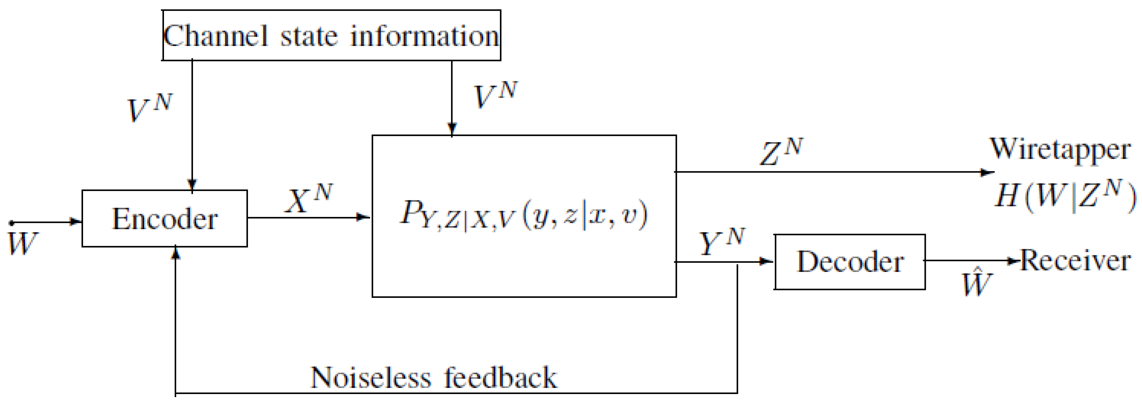
2.1. Definitions of the Model of Figure 1

Let W, uniformly distributed over the alphabet $\mathcal{W}$, be the message sent by the transmitter. The components of the channel state sequence $V^N$ are independent and identically distributed. The probability of each component is $P_V\left(v\right)$. $V^N$ is independent of W. Let $Y^{i-1}$ ($2\le i\le N$) be the i-th time feedback from the legitimate receiver to the transmitter. For the noncausal case, the i-th time channel encoder $f_i$ is a (stochastic) mapping:

$$f_i:\mathcal{W}\times {\mathcal{Y}}^{i-1}\times {\mathcal{V}}^N\to {\mathcal{X}}_i,$$

(4)

where $f_i(w,y^{i-1},v^N)=x_i\in \mathcal{X}$, $w\in \mathcal{W}$, $y^{i-1}\in {\mathcal{Y}}^{i-1}$ and $v^N\in {\mathcal{V}}^N$. For the causal case, the i-th time channel encoder $f_i$ is a (stochastic) mapping:

$$f_i:\mathcal{W}\times {\mathcal{Y}}^{i-1}\times {\mathcal{V}}^i\to {\mathcal{X}}_i,$$

(5)

where $f_i(w,y^{i-1},v^i)=x_i\in \mathcal{X}$, $w\in \mathcal{W}$, $y^{i-1}\in {\mathcal{Y}}^{i-1}$ and $v^i\in {\mathcal{V}}^i$. Here, note that for the causal case, $V_i$ is independent of $(Y^{i-1},W,V_{i+1}^N,Z^{i-1})$.

The channel is discrete memoryless, and its transition probability is given by:

$$P_{Z^N,Y^N|X^N,V^N}(z^N,y^N|x^N,v^N)=\prod _{i=1}^N{P}_{Z,Y|X,V}(z_i,y_i|x_i,v_i),$$

(6)

where $x_i\in \mathcal{X}$, $v_i\in \mathcal{V}$, $y_i\in \mathcal{Y}$ and $z_i\in \mathcal{Z}$.

The wiretapper’s equivocation about the message W is denoted by:

$$\Delta =\frac{1}{N}H\left(W\right|Z^N).$$

(7)

The decoder $f_D$ is a function that maps a received sequence of N channel outputs to the messages set:

$$f_D:{\mathcal{Y}}^N\to \mathcal{W}.$$

(8)

We denote the probability of error $P_e$ by $Pr\{W\ne \widehat{W}\}$.

Given a pair $(R,R_e)$ ($R,R_e>0$), it is said to be achievable if, for arbitrary small positive ϵ, there exists an encoding-decoding scheme, such that:

$$\underset{N\to \infty }{lim}\frac{log\parallel \mathcal{W}\parallel }{N}=R,\underset{N\to \infty }{lim}\Delta \ge R_e,P_e\le ϵ.$$

(9)

The set ${\mathcal{R}}^{\left(nf\right)}$, which is composed of all achievable $(R,R_e)$ pairs, is called the capacity-equivocation region of the model of Figure 1 with noncausal CSI at the transmitter. An achievable rare $C_s^{\left(nf\right)}$, which is denoted by:

$$C_s^{\left(nf\right)}=\underset{(R,R_e=R)\in {\mathcal{R}}^{\left(nf\right)}}{max}R,$$

(10)

is called the secrecy capacity of the model of Figure 1 with noncausal CSI at the transmitter.

Analogously, let ${\mathcal{R}}^{\left(cf\right)}$ be the capacity-equivocation region of the model of Figure 1 with causal CSI at the transmitter and $C_s^{\left(cf\right)}$, which is denoted by:

$$C_s^{\left(cf\right)}=\underset{(R,R_e=R)\in {\mathcal{R}}^{\left(cf\right)}}{max}R,$$

(11)

be the secrecy capacity of the model of Figure 1 with causal CSI at the transmitter.

2.2. Main Result of the Model of Figure 1

The following Theorem 1 characterizes the capacity-equivocation region ${\mathcal{R}}^{\left(nf\right)}$ of the model of Figure 1 with noncausal CSI at the transmitter; see the following.

Theorem 1. A single-letter characterization of the region ${\mathcal{R}}^{\left(nf\right)}$ is as follows,

$$\begin{array}{ccc}& & {\mathcal{R}}^{\left(nf\right)}=\{(R,R_e):0\le R_e\le R,\hfill \\ & & 0\le R\le I(K;Y)-I(K;V),\hfill \\ & & R_e\le H\left(Y\right|Z)\},\hfill \end{array}$$

for some distribution:

$$\begin{array}{ccc}& & P_{KVXYZ}(k,v,x,y,z)=P_{ZY|XV}(z,y|x,v)P_{X|KV}\left(x\right|k,v)P_{KV}(k,v),\hfill \end{array}$$

which implies the Markov chain $K\to (X,V)\to (Y,Z)$.

Proof. See Section A and Section B.  ☐

Remark 1.

• The range of the random variable K satisfies $\parallel \mathcal{K}\parallel \le \parallel \mathcal{X}\parallel \parallel \mathcal{V}\parallel +1$. The proof is standard and easily obtained by using the support lemma (see [15]), and thus, we omit the proof here.
• Corollary 1. The secrecy capacity $C_s^{\left(nf\right)}$ satisfies:

  $$C_s^{\left(nf\right)}=\underset{P_{X|KV}{P}_{KV}}{max}min\{I(K;Y)-I(K;V),H\left(Y\right|Z)\}.$$

  (12)
  Proof. Substituting $R_e=R$ into the region ${\mathcal{R}}^{\left(nf\right)}$ in Theorem 1, we have:

  $$\begin{array}{ccc}\hfill R& \le & I(K;Y)-I(K;V),\hfill \end{array}$$

  (13)

  $$\begin{array}{ccc}\hfill R& \le & H\left(Y\right|Z),\hfill \end{array}$$

  (14)

  By using (10), (13) and (14), Formula (12) is achieved; thus, the proof is completed. ☐
• Here, note that if $Z^N$ is a degraded version of $Y^N$ (which implies the existence of the Markov chain $K\to (X,V)\to Y\to Z$), the capacity-equivocation region ${\mathcal{R}}^{\left(nf\right)}$ still holds. The proof of this degraded case is along the lines of the proof of Theorem 1, and thus, we omit the proof here. In [10,12], an achievable rate-equivocation region ${\mathcal{R}}_i^n$ is provided for the wiretap channel with noncausal CSI, and it is given by:

  $$\begin{array}{ccc}& & {\mathcal{R}}_i^n=\{(R,R_e):R_e\le R,\hfill \\ & & R\le I(K;Y)-I(K;V),R_e\le I(K;Y)-I(K;Z)\},\hfill \end{array}$$

  where the joint probability distribution $P_{KVXYZ}(k,v,x,y,z)$ of ${\mathcal{R}}_i^n$ satisfies:

  $$\begin{array}{ccc}& & P_{KVXYZ}(k,v,x,y,z)=P_{Z|Y}\left(z\right|y)P_{Y|XV}\left(y\right|x,v)P_{X|KV}\left(x\right|k,v)P_{KV}(k,v).\hfill \end{array}$$

  Here, note that:

  $$\begin{array}{c}\hfill \begin{array}{cc}\hfill I(K;Y)-I(K;Z)& =H\left(K\right|Z)-H(K\left|Y\right)\hfill \\ & \stackrel{\left(a\right)}{=}H\left(K\right|Z)-H\left(K\right|Y,Z)=I(K;Y|Z)\hfill \\ & \le H\left(Y\right|Z),\hfill \end{array}\end{array}$$

  (15)

  where (a) is from $K\to Y\to Z$. Therefore, it is easy to see that the achievable rate-equivocation region ${\mathcal{R}}_i^n$ of [10] and [12] is enhanced by using this noiseless feedback.

The following Theorem 2 characterizes the capacity-equivocation region ${\mathcal{R}}^{\left(cf\right)}$ of the model of Figure 1 with causal CSI at the transmitter; see the following.

Theorem 2. A single-letter characterization of the region ${\mathcal{R}}^{\left(cf\right)}$ is as follows,

$$\begin{array}{ccc}& & {\mathcal{R}}^{\left(cf\right)}=\{(R,R_e):0\le R_e\le R,\hfill \\ & & 0\le R\le I(K;Y),\hfill \\ & & R_e\le H\left(Y\right|Z)\},\hfill \end{array}$$

for some distribution:

$$\begin{array}{ccc}& & P_{KVXYZ}(k,v,x,y,z)=P_{YZ|XV}(y,z|x,v)P_{X|KV}\left(x\right|k,v)P_K\left(k\right)P_V\left(v\right).\hfill \end{array}$$

which implies the Markov chain $K\to (X,V)\to (Y,Z)$ and the fact that V is independent of K.

Proof.

• Proof of the converse: Using the fact that $V_i$ is independent of $Y^{i-1}$ and $Z^{i-1}$, the converse proof of Theorem 2 is along the lines of that of Theorem 1 (see Section A), and thus, we omit the proof here.
• Proof of the achievability: The achievability proof of Theorem 2 is along the lines of the achievability proof of Theorem 1 (see Section B), and the only difference is that for the causal case, there is no need to use the binning technique. Thus, we omit the proof here.

The proof of Theorem 2 is completed.  ☐

Remark 2.

• The range of the auxiliary random variable K satisfies $\parallel \mathcal{K}\parallel \le \parallel \mathcal{X}\parallel \parallel \mathcal{V}\parallel$. The proof is standard and easily obtained by using the support lemma (see p. 310 of [16]), and thus, we omit the proof here.
• Corollary 2. The secrecy capacity $C_s^{\left(cf\right)}$ satisfies:

  $$C_s^{\left(cf\right)}=\underset{P_{X|KV}{P}_K}{max}min\{I(K;Y),H\left(Y\right|Z)\}.$$

  (16)
  Proof. Proof of (16): Substituting $R_e=R$ into the region ${\mathcal{R}}^{\left(cf\right)}$, we have:

  $$\begin{array}{ccc}\hfill R& \le & I(K;Y),\hfill \end{array}$$

  (17)

  $$\begin{array}{ccc}\hfill R& \le & H\left(Y\right|Z),.\hfill \end{array}$$

  (18)

  By using (11), (17) and (18), Formula (16) is achieved; thus, the proof is completed. ☐
• Here, note that if $Z^N$ is a degraded version of $Y^N$, the capacity-equivocation region ${\mathcal{R}}^{\left(cf\right)}$ still holds. The proof of this degraded case is along the lines of the proof of Theorem 2, and thus, we omit the proof here. In [12], an achievable rate-equivocation region ${\mathcal{R}}_i^c$ is provided for the wiretap channel with causal CSI, and it is given by:

  $$\begin{array}{ccc}& & {\mathcal{R}}_i^c=\{(R,R_e):R_e\le R,\hfill \end{array}$$

  $$\begin{array}{ccc}& & R\le I(K;Y),R_e\le I(K;Y)-I(K;Z)\},\hfill \end{array}$$

  (19)

  where the joint probability distribution $P_{KVXYZ}(k,v,x,y,z)$ of ${\mathcal{R}}_i^c$ satisfies:

  $$\begin{array}{ccc}& & P_{KVXYZ}(k,v,x,y,z)=P_{Z|Y}\left(z\right|y)P_{Y|XV}\left(y\right|x,v)P_{X|KV}\left(x\right|k,v)P_K\left(k\right)P_V\left(v\right).\hfill \end{array}$$

  By using (15), it is easy to see that the achievable rate-equivocation region ${\mathcal{R}}_i^c$ is enhanced by using this noiseless feedback.

3. Examples of the Model of Figure 1

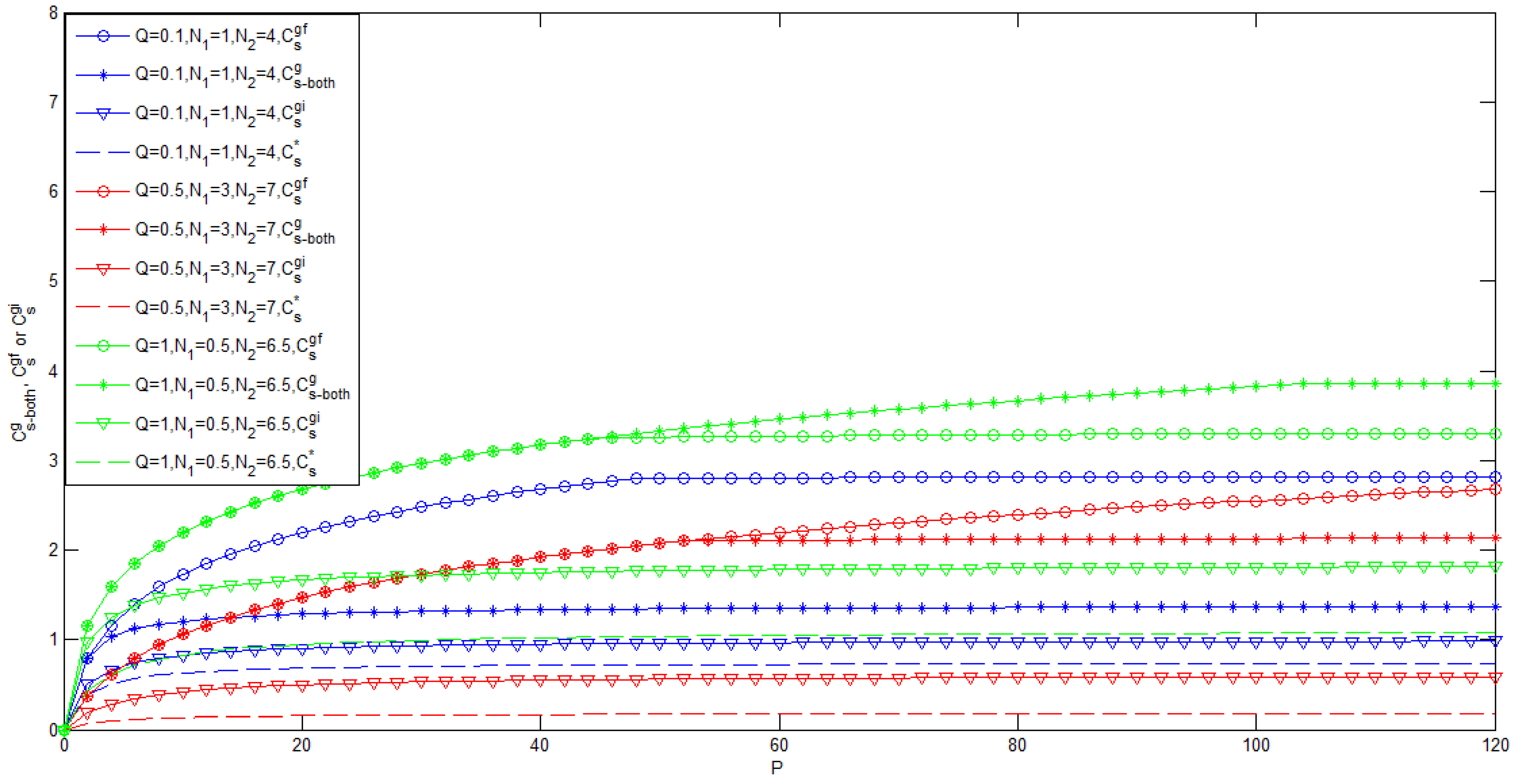
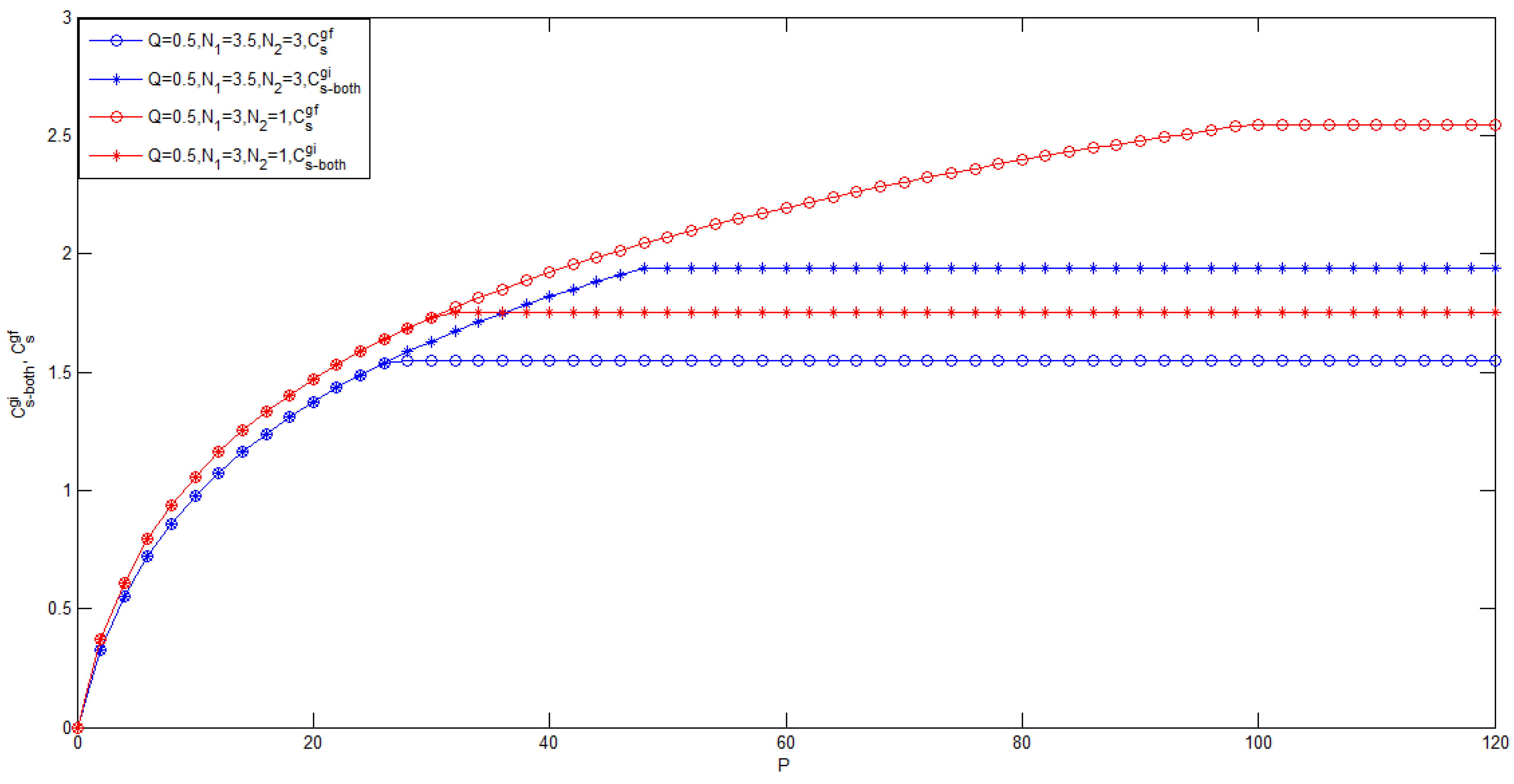
3.1. Gaussian Case of the Model of Figure 1 with Noncausal CSI at the Transmitter

For the Gaussian case of the model of Figure 1 with noncausal CSI at the transmitter, the i-th time ($1\le i\le N$) channel inputs and outputs are given by:

$$Y_i=X_i+V_i+Z_{1,i},Z_i=X_i+V_i+Z_{2,i},$$

(20)

where $V_i\sim \mathcal{N}(0,Q)$, $Z_{1,i}\sim \mathcal{N}(0,N_1)$ and $Z_{2,i}\sim \mathcal{N}(0,N_2)$. Here, note that $V_i$, $Z_{1,i}$ and $Z_{2,i}$ are independent random variables, $X_i$ is independent of $Z_{1,i}$ and $Z_{2,i}$ and $\frac{1}{N}{\sum }_{i=1}^{N}E\left(X_i^2\right)\le P$. The noise $V_i$ is non-causally known by the transmitter. The following Theorem 3 shows the secrecy capacity of the Gaussian case of the model of Figure 1 with noncausal CSI at the transmitter.

Theorem 3. For the Gaussian case of the model of Figure 1 with noncausal CSI at the transmitter, the secrecy capacity $C_s^{gf}$ is characterized in the following two cases.

Case 1: If $N_1\le N_2$, the secrecy capacity $C_s^{gf}$ is given by:

$$\begin{array}{cc}\hfill C_s^{gf}& =\underset{\alpha }{max}min\left\{\begin{array}{c}\frac{1}{2}ln\frac{(P+Q+N_1)(P+{\alpha }^{2}Q)}{PQ{(1-\alpha )}^2+N(P+{\alpha }^{2}Q)}-\frac{1}{2}ln\frac{P+{\alpha }^{2}Q}{P},\hfill \\ \frac{1}{2}ln\frac{2\pi e(P+Q+N_1)(N_2-N_1)}{P+Q+N_2}\hfill \end{array}\right\}\hfill \\ & =min\{\frac{1}{2}ln(1+\frac{P}{N_1}),\frac{1}{2}ln\frac{2\pi e(P+Q+N_1)(N_2-N_1)}{P+Q+N_2}\},\hfill \end{array}$$

(21)

where the maximum is achieved when $\alpha =\frac{P}{P+N_1}$.

Case 2: If $N_1>N_2$, the secrecy capacity $C_s^{gf}$ is given by:

$$\begin{array}{ccc}\hfill C_s^{gf}& =& min\{\frac{1}{2}ln(1+\frac{P}{N_1}),\frac{1}{2}ln2\pi e(N_1-N_2)\}.\hfill \end{array}$$

(22)

Remark 3.

If $N_1\le N_2$, the relationship of the channel inputs and outputs defined in (20) can be equivalently characterized by:

$$Y_i=X_i+V_i+Z_{1,i},Z_i=X_i+V_i+Z_{1,i}+Z_{2,i}^{*},$$

(23)

where $Z_{2,i}^{*}\sim \mathcal{N}(0,N_2-N_1)$, and it is independent of $Z_{1,i}$. Similar to the determination of the capacity region of the Gaussian broadcast channel (pp. 117–118 of [17]), the relationship (23) implies that there exists a Markov chain $(X_i,V_i)\to Y_i\to Z_i$, i.e., the Gaussian case of the model of Figure 1 reduces to a degraded model of Figure 1.

Analogously, if $N_1>N_2$, the relationship of the channel inputs and outputs defined in (20) can be equivalently characterized by:

$$Y_i=X_i+V_i+Z_{1,i}^{*}+Z_{2,i},Z_i=X_i+V_i+Z_{2,i},$$

(24)

where $Z_{1,i}^{*}\sim \mathcal{N}(0,N_1-N_2)$, and it is independent of $Z_{2,i}$, $X_i$ and $V_i$. The relationship (24) implies that there exists a Markov chain $(X_i,V_i)\to Z_i\to Y_i$ in the Gaussian case of the model of Figure 1.

Proof. For the direct part of Theorem 3, like [18] and [10], the achievability of $C_s^{gf}$ is proven by substituting $K=X+\alpha V$, $X\sim \mathcal{N}(0,P)$, $V\sim \mathcal{N}(0,Q)$ and the fact that X is independent of V in Theorem 1; the details of the proof are omitted in this paper. Here, note that the calculation of $I(K;Y)-I(K;V)$ is exactly the same as that of the dirty paper channel (page 440 of [18]), and it is easy to see that the maximum of $I(K;Y)-I(K;V)$ is achieved when $\alpha =\frac{P}{P+N_1}$.

For the converse part of Theorem 3, note that the transmitter-receiver channel is Costa’s dirty paper channel [18]; thus, the secrecy capacity is upper bounded by the capacity of the dirty paper channel, i.e., $C_s^{gf}\le \frac{1}{2}ln(1+\frac{P}{N_1})$. Now, it remains to show $C_s^{gf}\le \frac{1}{2}ln\frac{2\pi e(P+Q+N_1)(N_2-N_1)}{P+Q+N_2}$ for $N_1\le N_2$ and $C_s^{gf}\le \frac{1}{2}ln2\pi e(N_1-N_2)$ for $N_1>N_2$; see the following.

Proof of $C_s^{gf}\le \frac{1}{2}ln\frac{2\pi e(P+Q+N_1)(N_2-N_1)}{P+Q+N_2}$ for $N_1\le N_2$:

First, note that:

$$\begin{array}{cc}\hfill \frac{1}{N}H\left(W\right|Z^N)& \stackrel{\left(a\right)}{\le }\frac{1}{N}(I(W;Y^N|Z^N)+\delta \left(P_e\right))\hfill \\ & \le \frac{1}{N}\sum _{i=1}^{N}h\left(Y_i\right|Z_i)+\frac{\delta \left(P_e\right)}{N},\hfill \end{array}$$

(25)

where (a) is from Fano’s inequality. The conditional differential entropy $h\left(Y_i\right|Z_i)$ in (25) is bounded by:

$$\begin{array}{cc}\hfill h\left(Y_i\right|Z_i)& =h(Y_i,Z_i)-h\left(Z_i\right)\hfill \\ & =h\left(Z_i\right|Y_i)+h\left(Y_i\right)-h\left(Z_i\right)\hfill \\ & \stackrel{\left(1\right)}{=}h(X_i+V_i+Z_{1,i}+Z_{2,i}^{*}|X_i+V_i+Z_{1,i})+h(X_i+V_i+Z_{1,i})-h(X_i+V_i+Z_{1,i}+Z_{2,i}^{*})\hfill \\ & \stackrel{\left(2\right)}{=}h\left(Z_{2,i}^{*}\right)+h(X_i+V_i+Z_{1,i})-h(X_i+V_i+Z_{1,i}+Z_{2,i}^{*})\hfill \\ & \stackrel{\left(3\right)}{\le }h\left(Z_{2,i}^{*}\right)+h(X_i+V_i+Z_{1,i})-\frac{1}{2}ln(e^{2h(X_i+V_i+Z_{1,i})}+e^{2h\left(Z_{2,i}^{*}\right)})\hfill \\ & =h\left(Z_{2,i}^{*}\right)+\frac{1}{2}ln\left(e^{2h(X_i+V_i+Z_{1,i})}\right)-\frac{1}{2}ln(e^{2h(X_i+V_i+Z_{1,i})}+e^{2h\left(Z_{2,i}^{*}\right)})\hfill \\ & \stackrel{\left(4\right)}{=}\frac{1}{2}ln\left(2\pi e(N_2-N_1)\right)+\frac{1}{2}ln\frac{e^{2h(X_i+V_i+Z_{1,i})}}{e^{2h(X_i+V_i+Z_{1,i})}+2\pi e(N_2-N_1)}\hfill \\ & \stackrel{\left(5\right)}{\le }\frac{1}{2}ln\left(2\pi e(N_2-N_1)\right)+\frac{1}{2}ln\frac{2\pi e(P+Q+N_1)}{2\pi e(P+Q+N_1)+2\pi e(N_2-N_1)}\hfill \\ & =\frac{1}{2}ln\frac{2\pi e(N_2-N_1)(P+Q+N_1)}{P+Q+N_2},\hfill \end{array}$$

(26)

where (1) is from Definition (23), (2) is from the fact that $Z_{2,i}^{*}$ is independent of $X_i$, $V_i$ and $Z_{1,i}$, (3) is from the entropy power inequality $e^{2h(X_i+V_i+Z_{1,i}+Z_{2,i}^{*})}\ge e^{2h(X_i+V_i+Z_{1,i})}+e^{2h\left(Z_{2,i}^{*}\right)}$ (see [19]), (4) is from the fact that the differential entropy of a Gaussian distributed random variable X is $h\left(X\right)=\frac{1}{2}ln\left(2\pi eD\left(X\right)\right)$ (here, $D\left(X\right)$ is the variance of the Gaussian random variable X) and (5) is from $\frac{1}{2}ln\frac{e^{2h(X_i+V_i+Z_{1,i})}}{e^{2h(X_i+V_i+Z_{1,i})}+2\pi e(N_2-N_1)}$ increasing while $h(X_i+V_i+Z_{1,i})$ is increasing and the fact that $h(X_i+V_i+Z_{1,i})\le \frac{1}{2}ln\left(2\pi e(P+Q+N_1)\right)$ (here, note that “=” is achieved if $X_i\sim \mathcal{N}(0,P)$).

Substituting (26) into (25), we have:

$$\begin{array}{cc}\hfill \frac{1}{N}H\left(W\right|Z^N)& \le \frac{1}{N}\sum _{i=1}^N\frac{1}{2}ln\frac{2\pi e(N_2-N_1)(P+Q+N_1)}{P+Q+N_2}+\frac{\delta \left(P_e\right)}{N}\hfill \\ & =\frac{1}{2}ln\frac{2\pi e(N_2-N_1)(P+Q+N_1)}{P+Q+N_2}+\frac{\delta \left(P_e\right)}{N}.\hfill \end{array}$$

(27)

Substituting $P_e\le ϵ$ into (27) and letting $N\to \infty$, it is easy to see that $C_s^{gf}\le \frac{1}{2}ln\frac{2\pi e(P+Q+N_1)(N_2-N_1)}{P+Q+N_2}$ for $N_1\le N_2$.

Proof of $C_s^{gf}\le \frac{1}{2}ln2\pi e(N_1-N_2)$ for $N_1>N_2$:

For the case $N_1>N_2$, the conditional differential entropy $h\left(Y_i\right|Z_i)$ in (25) can be bounded by:

$$\begin{array}{cc}\hfill h\left(Y_i\right|Z_i)& \stackrel{\left(a\right)}{=}h(X_i+V_i+Z_{1,i}^{*}+Z_{2,i}|X_i+V_i+Z_{2,i})\hfill \\ & \stackrel{\left(b\right)}{=}h\left(Z_{1,i}^{*}\right)\hfill \\ & \stackrel{\left(c\right)}{=}\frac{1}{2}ln2\pi e(N_1-N_2),\hfill \end{array}$$

(28)

where (a) is from (24), (b) is from the fact that $Z_{1,i}^{*}$ is independent of $Z_{2,i}$, $X_i$ and $V_i$ and (c) is from the fact that the differential entropy of a Gaussian distributed random variable X is $h\left(X\right)=\frac{1}{2}ln\left(2\pi eD\left(X\right)\right)$ (here, $D\left(X\right)$ is the variance of the Gaussian random variable X). Substituting (28) and $P_e\le ϵ$ into (25) and letting $N\to \infty$, it is easy to see that $C_s^{gf}\le \frac{1}{2}ln2\pi e(N_1-N_2)$ for $N_1>N_2$. Thus, the converse part of Theorem 3 is proven. The proof of Theorem 3 is completed.  ☐

In [13] (p.2841, Theorem 3), Chia and El Gamal showed that if Y is less noisy than Z ($I(X;Y|V)\ge I(X;Z\left|V\right)$ for every $P_{X|V}\left(x\right|v)$), the secrecy capacity of the wiretap channel with CSI non-causally known by both the transmitter and the legitimate receiver is given by:

$$\begin{array}{ccc}& & C_{s-both}=\underset{p\left(x\right|v)}{max}min\{I(X;Y|V),I(X;Y|V)-I(X;Z|V)+H\left(V\right|Z)\}.\hfill \end{array}$$

Here, the $I(X;Z|V)-H(V\left|Z\right)$ in the above $C_{s-both}$ can be rewritten as follows.

$$\begin{array}{cc}\hfill I(X;Z|V)-H(V\left|Z\right)& =H\left(Z\right|V)-H(Z|X,V)-H\left(V\right|Z)\hfill \\ & =H(V,Z)-H\left(V\right)-H\left(Z\right|X,V)-H(V,Z)+H(Z)\hfill \\ & =H\left(Z\right)-H\left(V\right)-H\left(Z\right|X,V).\hfill \end{array}$$

(29)

Substituting (29) into $C_{s-both}$, we have:

$$\begin{array}{ccc}& & C_{s-both}=\underset{p\left(x\right|v)}{max}min\{I(X;Y|V),I(X;Y|V)-H\left(Z\right)+H\left(V\right)+H\left(Z\right|X,V)\}.\hfill \end{array}$$

(30)

On the other hand, for Z less noisy than Y ($I(X;Z|V)\ge I(X;Y\left|V\right)$ for every $P_{X|V}\left(x\right|v)$), Chia and El Gamal provided an achievable secrecy rate (lower bound on the secrecy capacity) for the wiretap channel with CSI non-causally known by both the transmitter and the legitimate receiver, and it is given by:

$$\begin{array}{ccc}& & C_{s-both}^i=\underset{p\left(x\right|v)}{max}min\{I(X;Y|V),H\left(V\right|Z,X)\}.\hfill \end{array}$$

(31)

The following Theorem 4 shows the results on the secrecy capacity of the Gaussian case of the wiretap channel with CSI non-causally known by both the transmitter and the legitimate receiver.

Theorem 4. For the Gaussian wiretap channel with part of the Gaussian noise non-causally known by both the transmitter and the legitimate receiver, the secrecy capacity $C_{s-both}^g$ is characterized by the following two cases.

Case 1: If $N_1\le N_2$, the secrecy capacity $C_{s-both}^g$ is given by:

$$\begin{array}{ccc}& & C_{s-both}^g=min\left\{\begin{array}{c}\frac{1}{2}ln(1+\frac{P}{N_1}),\hfill \\ \frac{1}{2}ln(1+\frac{P}{N_1})+\frac{1}{2}ln\left(2\pi eQ\right)-\frac{1}{2}ln\left(\frac{P+Q+N_2}{N_2}\right)\hfill \end{array}\right\}.\hfill \end{array}$$

(32)

Case 2: If $N_1>N_2$, a lower bound $C_{s-both}^{gi}$ on the secrecy capacity $C_{s-both}^g$ is given by:

$$\begin{array}{ccc}& & C_{s-both}^g\ge C_{s-both}^{gi}=min\{\frac{1}{2}ln\frac{2\pi eQ{N}_2}{Q+N_2},\frac{1}{2}ln(1+\frac{P}{N_1})\}.\hfill \end{array}$$

(33)

Remark 4.

For the Gaussian case, the conditional mutual information $I(X;Y|V)$ is calculated by using the fact that when the CSI is known by both the legitimate receiver and the transmitter, it can be simply subtracted off, which in effect reduces the channel to a Gaussian channel with no CSI, i.e., $I(X;Y|V)=\frac{1}{2}ln(1+\frac{P}{N_1})$. Analogously, we have $I(X;Z|V)=\frac{1}{2}ln(1+\frac{P}{N_2})$. Then, it is easy to see that Y is less noisy than Z ($I(X;Z|V)\ge I(X;Y\left|V\right)$ for every $P_{X|V}\left(x\right|v)$), which can be further expressed by $N_1\le N_2$, and Z is less noisy than Y ($I(X;Z|V)\ge I(X;Y\left|V\right)$ for every $P_{X|V}\left(x\right|v)$), which can be further expressed by $N_1\ge N_2$.

Proof. The achievability proof of (32) and (33) is easily obtained by substituting $X\sim \mathcal{N}(0,P)$, $V\sim \mathcal{N}(0,Q)$ and (20) into (30) and (31), respectively. Now, it remains to prove the converse of (32); see the following.

The converse part of (32) is based on the converse proof of (30), (see p.2846, Proof of Theorem 2 of [13] and the left bottom and right top of page 2841 [13]). However, the converse proof of (30) is for the discrete memoryless case, and it needs to be further processed for the Gaussian case. Based on the converse proof of (30) [13] and the fact that $N_1\le N_2$, we have the following (34) and (35),

$$\begin{array}{cc}\hfill C_{s-both}^g& \le \frac{1}{N}\sum _{i=1}^N(I(X_i;Y_i|V_i)-I(X_i;Z_i|V_i)+h\left(V_i\right|Z_i))\hfill \\ & \stackrel{\left(1\right)}{=}\frac{1}{N}\sum _{i=1}^N(I(X_i;Y_i|V_i)-h\left(Z_i\right)+h\left(V_i\right)+h\left(Z_i\right|X_i,V_i))\hfill \\ & \stackrel{\left(2\right)}{=}\frac{1}{N}\sum _{i=1}^N(h(X_i+Z_{1,i}|V_i)-h\left(Z_{1,i}\right)-h\left(Z_i\right)+h\left(V_i\right)+h(Z_{1,i}+Z_{2,i}^{*}))\hfill \\ & \le \frac{1}{N}\sum _{i=1}^N(h(X_i+Z_{1,i})-h\left(Z_{1,i}\right)-h\left(Z_i\right)+h\left(V_i\right)+h(Z_{1,i}+Z_{2,i}^{*}))\hfill \\ & \stackrel{\left(3\right)}{=}\frac{1}{N}\sum _{i=1}^N(h(X_i+Z_{1,i})-\frac{1}{2}ln\left(2\pi e{N}_1\right)-h(X_i+V_i+Z_{1,i}+Z_{2,i}^{*})+\frac{1}{2}ln\left(2\pi eQ\right)\hfill \\ & +\frac{1}{2}ln\left(2\pi e{N}_2\right))\hfill \\ & \stackrel{\left(4\right)}{\le }\frac{1}{N}\sum _{i=1}^N(\frac{1}{2}ln\left(e^{2h(X_i+Z_{1,i})}\right)-\frac{1}{2}ln\left(2\pi e{N}_1\right)-\frac{1}{2}ln(e^{2h(X_i+Z_{1,i})}+e^{2h(V_i+Z_{2,i}^{*})})\hfill \\ & +\frac{1}{2}ln\left(2\pi eQ\right)+\frac{1}{2}ln\left(2\pi e{N}_2\right))\hfill \\ & \stackrel{\left(5\right)}{=}\frac{1}{N}\sum _{i=1}^N(\frac{1}{2}ln\left(e^{2h(X_i+Z_{1,i})}\right)-\frac{1}{2}ln\left(2\pi e{N}_1\right)-\frac{1}{2}ln(e^{2h(X_i+Z_{1,i})}+2\pi e(Q+N_2-N_1))\hfill \\ & +\frac{1}{2}ln\left(2\pi eQ\right)+\frac{1}{2}ln\left(2\pi e{N}_2\right))\hfill \\ & =\frac{1}{N}\sum _{i=1}^N(\frac{1}{2}ln\frac{e^{2h(X_i+Z_{1,i})}}{e^{2h(X_i+Z_{1,i})}+2\pi e(Q+N_2-N_1)}-\frac{1}{2}ln\left(2\pi e{N}_1\right)+\frac{1}{2}ln\left(2\pi eQ\right)+\frac{1}{2}ln\left(2\pi e{N}_2\right))\hfill \\ & \stackrel{\left(6\right)}{\le }\frac{1}{N}\sum _{i=1}^N(\frac{1}{2}ln\frac{2\pi e(P+N_1)}{2\pi e(P+N_1)+2\pi e(Q+N_2-N_1)}-\frac{1}{2}ln\left(2\pi e{N}_1\right)\hfill \\ & +\frac{1}{2}ln\left(2\pi eQ\right)+\frac{1}{2}ln\left(2\pi e{N}_2\right))\hfill \\ & =\frac{1}{2}ln(1+\frac{P}{N_1})+\frac{1}{2}ln\left(2\pi eQ\right)-\frac{1}{2}ln\left(\frac{P+Q+N_2}{N_2}\right),\hfill \end{array}$$

(34)

and:

$$\begin{array}{cc}\hfill C_{s-both}^g& \le \frac{1}{N}\sum _{i=1}^{N}I(X_i;Y_i|V_i)\hfill \\ & =\frac{1}{N}\sum _{i=1}^N(h\left(Y_i\right|V_i)-h\left(Y_i\right|V_i,X_i))\hfill \\ & \stackrel{\left(7\right)}{=}\frac{1}{N}\sum _{i=1}^N(h(X_i+Z_{1,i}|V_i)-h\left(Z_{1,i}\right))\hfill \\ & \le \frac{1}{N}\sum _{i=1}^N(h(X_i+Z_{1,i})-h\left(Z_{1,i}\right))\hfill \\ & \stackrel{\left(8\right)}{\le }\frac{1}{N}\sum _{i=1}^N(\frac{1}{2}ln\left(2\pi e(P+N_1)\right)-\frac{1}{2}ln\left(2\pi e{N}_1\right))\hfill \\ & =\frac{1}{2}ln(1+\frac{P}{N_1}),\hfill \end{array}$$

(35)

where (1) is from (29), (2) is from Definition (23) and $Z_{2,i}^{*}\sim \mathcal{N}(0,N_2-N_1)$, (3) is from the fact that the differential entropy of a Gaussian distributed random variable X is $h\left(X\right)=\frac{1}{2}ln\left(2\pi eD\left(X\right)\right)$ (here, $D\left(X\right)$ is the variance of the Gaussian random variable X), (4) is from the entropy power inequality $e^{2h(X_i+V_i+Z_{1,i}+Z_{2,i})}\ge e^{2h(X_i+Z_{1,i})}+e^{2h(V_i+Z_{2,i})}$ (see [19]), (5) is from $h(V_i+Z_{2,i})=\frac{1}{2}ln\left(2\pi e(Q+N_2)\right)$, (6) is from $\frac{1}{2}ln\frac{e^{2h(X_i+Z_{1,i})}}{e^{2h(X_i+Z_{1,i})}+2\pi e(Q+N_2)}$ increasing while $h(X_i+Z_{1,i})$ is increasing and the fact that $h(X_i+Z_{1,i})\le \frac{1}{2}ln\left(2\pi e(P+N_1)\right)$ (here, note that “=” is achieved if $X_i\sim \mathcal{N}(0,P)$), (7) is from Definition (23) and (8) is from $h(X_i+Z_{1,i})\le \frac{1}{2}ln\left(2\pi e(P+N_1)\right)$. Thus, the converse part of (32) is proven. The proof of Theorem 4 is completed.  ☐

Recall that for the degraded Gaussian wiretap channel with noncausal CSI at the transmitter ($(X,V)\to Y\to Z$), an achievable secrecy rate (a lower bound on the secrecy capacity) is provided [10]; see the following Theorem 5.

Theorem 5. For the Gaussian non-feedback model of Figure 1 with the condition that $N_1\le N_2$, an achievable secrecy rate $C_s^{gi}$ is denoted by:

$$\begin{array}{ccc}& & C_s^{gi}=\underset{0\le \alpha \le 1}{max}min\left\{\begin{array}{c}\frac{1}{2}ln\frac{(P+N_1)(P+{\alpha }^{2}Q)}{{\alpha }^{2}Q(P+N_1)+N_{1}P}-\frac{1}{2}ln\frac{P+{\alpha }^{2}Q}{P},\hfill \\ \frac{1}{2}ln\frac{(P+N_1)(P+{\alpha }^{2}Q)}{{\alpha }^{2}Q(P+N_1)+N_{1}P}-\frac{1}{2}ln\frac{(P+N_2)(P+{\alpha }^{2}Q)}{{\alpha }^{2}QP+N_2(P+{\alpha }^{2}Q)}\hfill \end{array}\right\}.\hfill \end{array}$$

Proof. The result is directly obtained from [10], and therefore, the proof is omitted here.  ☐

Remark 5.

• For the case $N_1\le N_2$, the relationship (20) of the channel inputs and outputs can be equivalently characterized by (23), which implies the Markov chain $(X,V)\to Y\to Z$.
• To the best of the authors’ knowledge, for the case $N_1>N_2$, the bounds on the secrecy capacity of the Gaussian wiretap channel with noncausal CSI at the transmitter are still unknown.

Finally, note that if the CSI is not available at the legitimate receiver, the wiretapper and the transmitter and there is no feedback link from the legitimate receiver to the transmitter, the Gaussian case of the model of Figure 1 (see (20)) reduces to the model of the Gaussian wiretap channel, where $V_i$ and $Z_{1,i}$ of (20) are the legitimate receiver’s channel noises and $V_i$ and $Z_{2,i}$ are the wiretapper’s channel noises. From [20], it is easy to see that the secrecy capacity $C_s^{*}$ of the Gaussian wiretap channel is given by:

$$C_s^{*}=\frac{1}{2}ln\frac{P+Q+N_1}{Q+N_1}-\frac{1}{2}ln\frac{P+Q+N_2}{Q+N_2}.$$

(36)

Comparing Theorem 3 to Theorem 4, we can conclude that if $N_1\le N_2$, for given P, $N_1$ and $N_2$, $C_s^{gf}$ is larger than $C_{s-both}^g$ if and only if:

$$Q\le \frac{N_1(N_2-N_1)(P+N_1)}{N_1^2+N_{2}P}.$$

(37)

For the case that $N_1>N_2$, we find that if $\frac{N_1}{2}<N_2<N_1$, for given P, $N_1$ and $N_2$, $C_s^{gf}$ is larger than $C_{s-both}^{gi}$ if and only if:

$$Q\le \frac{N_2(N_1-N_2)}{2N_2-N_1}.$$

(38)

If $N_2=\frac{N_1}{2}$, $C_s^{gf}$ is always larger than $C_{s-both}^{gi}$.

If $N_2<\frac{N_1}{2}$, for given P, $N_1$ and $N_2$, $C_s^{gf}$ is larger than $C_{s-both}^{gi}$ if and only if:

$$Q\ge \frac{N_2(N_1-N_2)}{2N_2-N_1}.$$

(39)

Figure 2. For $N_1\le N_2$, the relationships of $P-C_s^{gf}$, $P-C_{s-both}^g$, $P-C_s^{gi}$ and $P-C_s^{*}$ for several values of $N_1$, $N_2$ and Q.

For the case $N_1\le N_2$, Figure 2 plots the relationships of $P-C_s^{*}$, $P-C_s^{gi}$, $P-C_s^{gf}$ and $P-C_{s-both}^g$ for several values of $N_1$, $N_2$ and Q. It is easy to see that the noiseless feedback ($C_s^{gf}$), the CSI sharing scheme ($C_{s-both}^g$) and the CSI only available at the transmitter ($C_s^{gi}$) help to enhance the secrecy capacity $C_s^{*}$ of the Gaussian wiretap channel. Furthermore, we can see that both the noiseless feedback and the CSI sharing scheme perform better than the CSI only available at the transmitter. Moreover, when Q is small ($Q=0.1,0.5$), the noiseless feedback performs better than the CSI sharing scheme, and while Q is increasing ($Q=1$), the CSI sharing scheme is beginning to take advantage of the noiseless feedback.

For the case $N_1>N_2$, the following Figure 3 plots the relationships of $P-C_s^{gf}$ and $P-C_{s-both}^g$ for several values of $N_1$, $N_2$ and Q. Since $C_s^{*}=0$ for the case that $N_1>N_2$, both the noiseless feedback ($C_s^{gf}$) and the CSI sharing scheme ($C_{s-both}^{gi}$) enhance the secrecy capacity $C_s^{*}$ of the Gaussian wiretap channel. Moreover, we can see that for fixed Q, if the gap between the legitimate receiver’s channel noise variance $N_1$ and the wiretapper’s channel noise variance $N_2$ is large, the noiseless feedback performs better than the CSI sharing scheme, and vice versa.

Figure 3. For $N_1>N_2$, the relationships of $P-C_s^{gf}$ and $P-C_{s-both}^{gi}$ for several values of $N_1$, $N_2$ and Q.

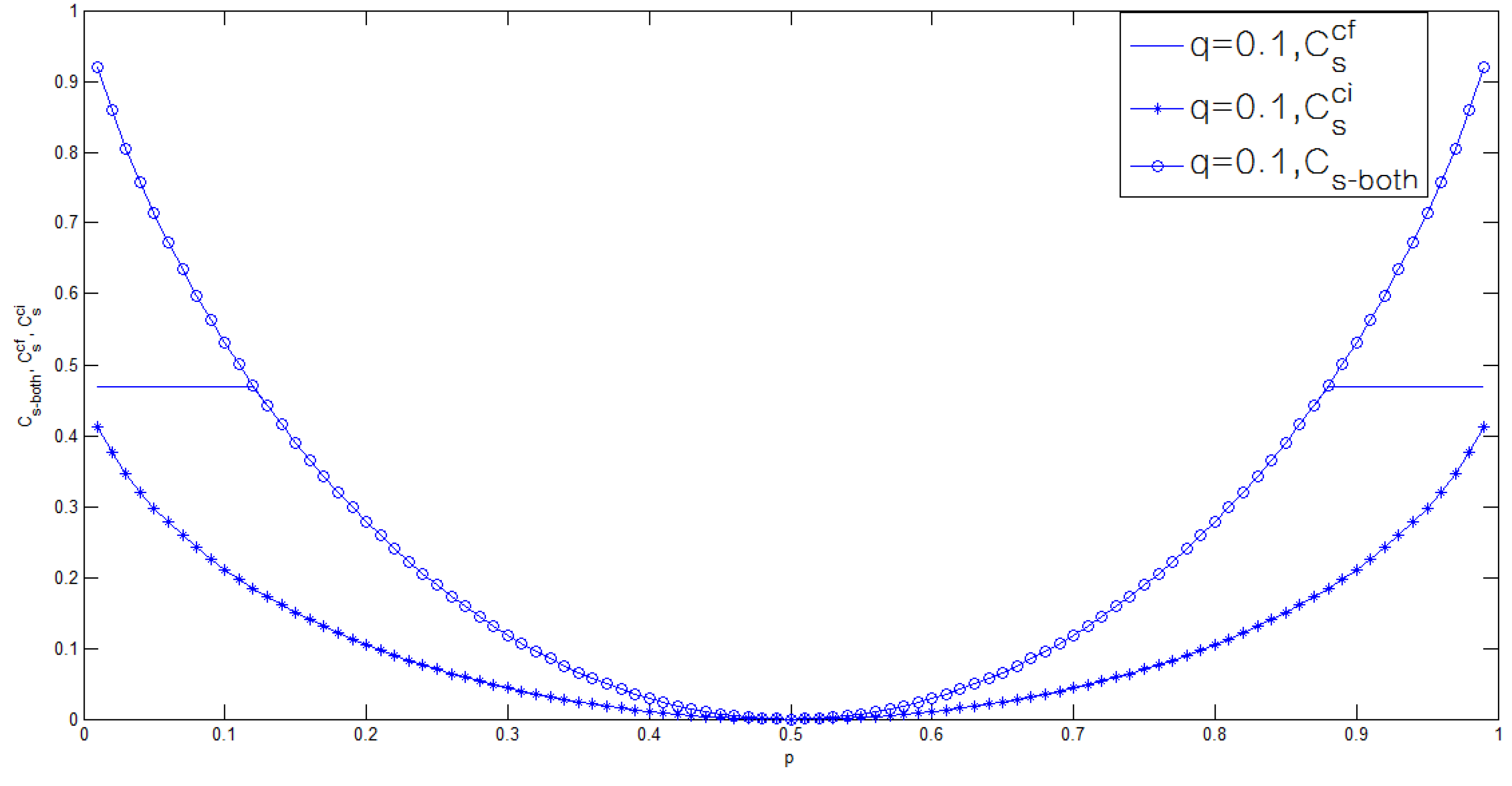
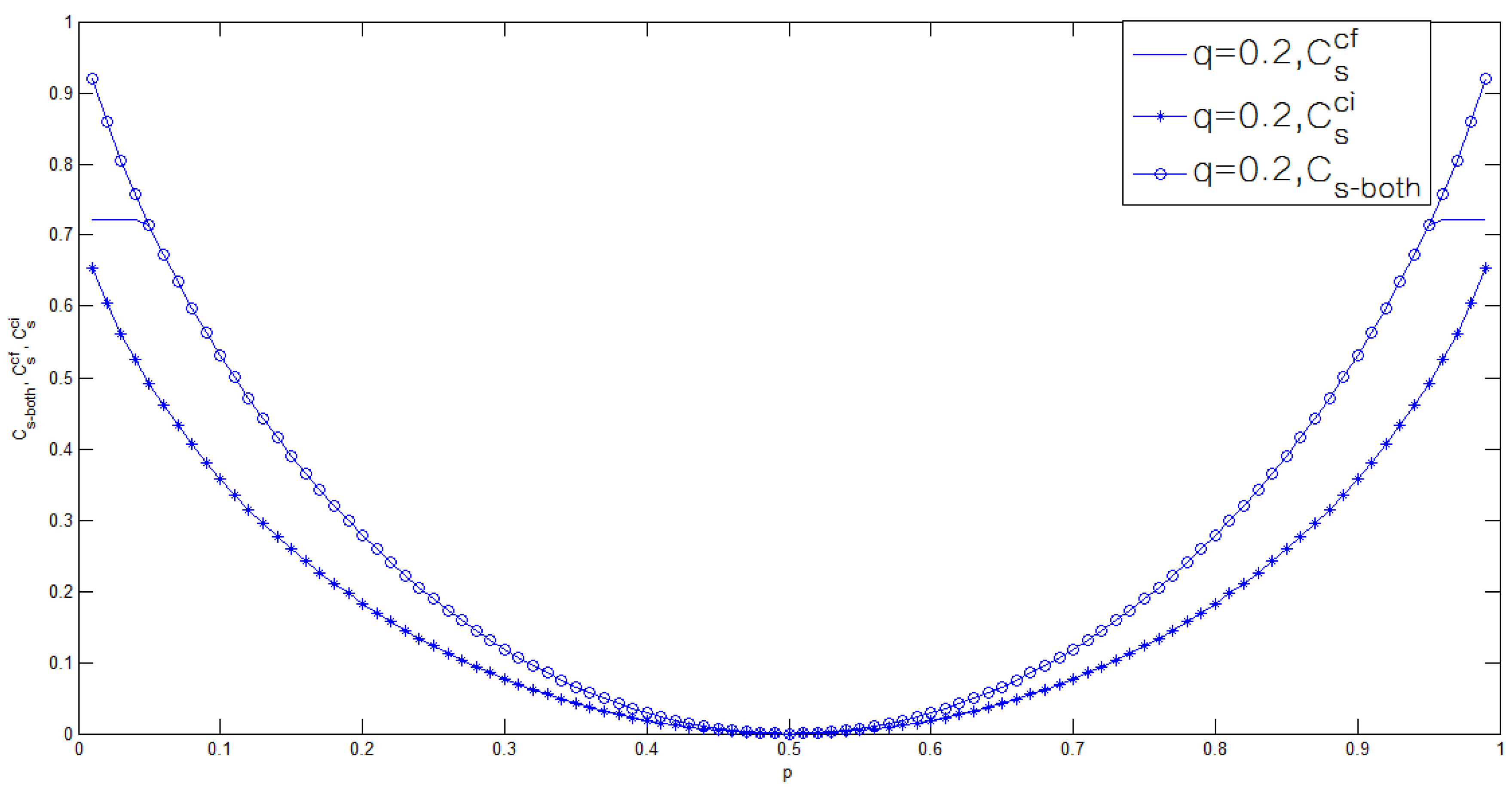
3.2. Binary Case of the Model of Figure 1

In this subsection, we calculate the secrecy capacity of a degraded binary case of the model of Figure 1 with causal CSI at the transmitter, where “degraded” means that there exists a Markov chain $(X,V)\to Y\to Z$.

Suppose that the random variable V is uniformly distributed over $\{0,1\}$, i.e., $p_V\left(0\right)=p_V\left(1\right)=\frac{1}{2}$. Meanwhile, the random variables X, Y and Z take values in $\{0,1\}$, and the wiretap channel is a BSC (binary symmetric channel) with crossover probability q. The transition probability of the main channel is defined as follows:

When $v=0$,

$$p_{Y|X,V}\left(y\right|x,v=0)=\left\{\begin{array}{cc}1-p,\hfill & \mathrm{if}y=x,\hfill \\ p,\hfill & \text{otherwise}.\hfill \end{array}\right.$$

(40)

When $v=1$,

$$p_{Y|X,V}\left(y\right|x,v=1)=\left\{\begin{array}{cc}p,\hfill & \mathrm{if}y=x,\hfill \\ 1-p,\hfill & \text{otherwise}.\hfill \end{array}\right.$$

(41)

From Remark 2, we know that the secrecy capacity for the model of Figure 1 with causal CSI at the transmitter is given by:

$$C_s^{\left(cf\right)}=\underset{P_K\left(k\right)P_{X|K,V}\left(x\right|k,v)}{max}min\{I(K;Y),H\left(Y\right|Z)\}$$

(42)

and the maximum achievable secrecy rate $C_s^{\left(ci\right)}$ of the wiretap channel with causal CSI [12] is given by:

$$C_s^{\left(ci\right)}=\underset{P_K\left(k\right)P_{X|K,V}\left(x\right|k,v)}{max}(I(K;Y)-I(K;Z)),$$

(43)

where (43) is from (19).

In addition, from ([13], Theorem 3), we know that the secrecy capacity $C_{s-both}$ of the wiretap channel with CSI causally or non-causally at both the transmitter and the legitimate receiver is given by:

$$C_{s-both}=\underset{P_{X|V}\left(x\right|v)}{max}min\{I(X;Y|V)-I(X;Z|V)+H\left(V\right|Z),I(X;Y|V)\}.$$

(44)

It remains to calculate $C_s^{\left(cf\right)}$, $C_s^{\left(ci\right)}$ and $C_{s-both}$; see the following.

The calculation of $C_s^{\left(cf\right)}$ and $C_s^{\left(ci\right)}$:

Let K take values in $\{0,1\}$. The probability of K is defined as follows. $p_K\left(0\right)=\alpha$, and $p_K\left(1\right)=1-\alpha$. Define the conditional probability mass function $p_{X|K,V}$ as follows.

$p_{X|K,V}\left(0\right|0,0)={\beta }_1$, $p_{X|K,V}\left(1\right|0,0)=1-{\beta }_1$, $p_{X|K,V}\left(0\right|0,1)={\beta }_2$, $p_{X|K,V}\left(1\right|0,1)=1-{\beta }_2$,

$p_{X|K,V}\left(0\right|1,0)={\beta }_3$, $p_{X|K,V}\left(1\right|1,0)=1-{\beta }_3$, $p_{X|K,V}\left(0\right|1,1)={\beta }_4$, $p_{X|K,V}\left(1\right|1,1)=1-{\beta }_4$.

The joint probability mass functions $p_{KY}$ is calculated by:

$$\begin{array}{cc}\hfill p_{KY}(k,y)& =\sum _{x,v}{p}_{KYXV}(k,y,x,v)\hfill \\ & =\sum _{x,v}{p}_{Y|XV}\left(y\right|x,v)p_{X|K,V}\left(x\right|k,v)p_K\left(k\right)p_V\left(v\right).\hfill \end{array}$$

(45)

Then, we have:

$$p_{KY}(0,0)=\frac{\alpha }{2}[1-({\beta }_1-{\beta }_2)(1-2p)],$$

(46)

$$p_{KY}(0,1)=\frac{\alpha }{2}[1+({\beta }_1-{\beta }_2)(1-2p)],$$

(47)

$$p_{KY}(1,0)=\frac{\alpha }{2}[1-({\beta }_3-{\beta }_4)(1-2p)],$$

(48)

$$p_{KY}(1,1)=\frac{\alpha }{2}[1+({\beta }_3-{\beta }_4)(1-2p)].$$

(49)

By calculating, we have:

$$C_s^{\left(cf\right)}=min\{1-h\left(p\right),h\left(q\right)\},$$

(50)

and:

$$C_s^{\left(ci\right)}=h(p+q-2pq)-h\left(p\right),$$

(51)

where $h\left(x\right)=-xlogx-(1-x)log(1-x)$ and $0\le x\le 1$.

The calculation of $C_{s-both}$:

Define $p_{X|V}\left(0\right|0)=\alpha$, $p_{X|V}\left(1\right|0)=1-\alpha$, $p_{X|V}\left(0\right|1)=\beta$, $p_{X|V}\left(1\right|1)=1-\beta$.

By calculating, $C_{s-both}$ is given by:

$$C_{s-both}=min\{1-h\left(p\right),1-h\left(p\right)+h(p+q-2pq)\}=1-h\left(p\right).$$

(52)

The following Figure 4, Figure 5 and Figure 6 show $C_s^{\left(cf\right)}$, $C_s^{\left(ci\right)}$ and $C_{s-both}$ for several values of q. Here, note that the noise of the wiretap channel is increasing while q is increasing. It is easy to see that when $q<0.5$, $C_{s-both}$ and $C_s^{\left(cf\right)}$ are always larger than $C_s^{\left(ci\right)}$, i.e., both the noiseless feedback (the model of this paper) and the shared CSI [13] help to enhance the security of the wiretap channel with causal CSI at the transmitter. When $q=0.5$, there is no wiretapper in the channel; thus, $C_s^{\left(cf\right)}=C_s^{\left(ci\right)}=C_{s-both}=1-h\left(p\right)$.

Moreover, from Figure 4, Figure 5 and Figure 6, we see that the noiseless feedback performs no better than the shared CSI. However, when q is large enough (satisfying $h\left(q\right)\ge 1-h\left(p\right)$), the two ways perform the same.

Figure 4. The $C_s^{\left(cf\right)}$, $C_s^{\left(ci\right)}$ and $C_{s-both}$ for $q=0.1$.

Figure 5. The $C_s^{\left(cf\right)}$, $C_s^{\left(ci\right)}$ and $C_{s-both}$ for $q=0.2$.

Figure 6. The $C_s^{\left(cf\right)}$, $C_s^{\left(ci\right)}$ and $C_{s-both}$ for $q=0.5$.

4. Conclusions

In this paper, we study the general wiretap channel with CSI and noiseless feedback, where the CSI is available at the transmitter in a noncausal or causal manner. Both the capacity-equivocation region and the secrecy capacity are determined for the noncausal and causal cases, and the results are further explained via Gaussian and binary examples. For the Gaussian example, we show that both the noiseless feedback and the CSI sharing scheme [13] help to enhance the security of the Gaussian wiretap channel. Moreover, we show that in some particular cases, the noiseless feedback performs even better than the CSI sharing scheme [13]. For the degraded binary example, we also find that the noiseless feedback enhances the security of the wiretap channel with causal CSI. Unlike the Gaussian example, we find that the noiseless feedback always performs no better than the CSI sharing scheme [13].

References

1. Ahlswede, R.; Cai, N. Transmission, Identification and Common Randomness Capacities for Wire-Tap Channels with Secure Feedback from the Decoder. In General Theory of Information Transfer and Combinatorics; Springer-Verlag: Berlin/Heidelberg, Germany, 2006; Volume 4123, pp. 258–275. [Google Scholar]
2. Dai, B.; Vinck, A.J.H.; Luo, Y.; Zhuang, Z. Capacity region of non-degraded wiretap channel with noiseless feedback. In Proceedings of 2012 IEEE International Symposium on Information Theory, Cambridge, MA, USA, 1–6 July 2012.
3. Wyner, A.D. The wire-tap channel. Bell Syst. Tech. J. 1975, 54, 1355–1387. [Google Scholar] [CrossRef]
4. Ardestanizadeh, E.; Franceschetti, M.; Javidi, T.; Kim, Y. Wiretap channel with secure rate-limited feedback. IEEE Trans. Inf. Theory 2009, 55, 5353–5361. [Google Scholar] [CrossRef]
5. Lai, L.; El Gamal, H.; Poor, H.V. The wiretap channel with feedback: Encryption over the channel. IEEE Trans. Inf. Theory 2008, 54, 5059–5067. [Google Scholar] [CrossRef]
6. He, X.; Yener, A. The role of feedback in two-way secure communication. IEEE Trans. Inf. Theory 2013, 59, 8115–8130. [Google Scholar] [CrossRef]
7. Bassi, G.; Piantanida, P.; Shamai, S. On the capacity of the wiretap channel with generalized feedback. In Processdings of 2015 IEEE International Symposium on Information Theory, Hong Kong, China, 14–19 June 2015.
8. Mitrpant, C.; Vinck, A.J.H.; Luo, Y. An achievable region for the gaussian wiretap channel with side information. IEEE Trans. Inf. Theory 2006, 52, 2181–2190. [Google Scholar] [CrossRef]
9. El-Halabi, M.; Liu, T.; Georghiades, C.N.; Shamai, S. Secret writing on dirty paper: A deterministic view. IEEE Trans. Inf. Theory 2012, 58, 3419–3429. [Google Scholar] [CrossRef]
10. Chen, Y.; Vinck, A.J.H. Wiretap channel with side information. IEEE Trans. Inf. Theory 2008, 54, 395–402. [Google Scholar] [CrossRef]
11. Gel’fand, S.I.; Pinsker, M.S. Coding for channel with random parameters. Probl. Control Inf. Theory 1980, 9, 19–31. [Google Scholar]
12. Dai, B.; Luo, Y. Some new results on wiretap channel with side information. Entropy 2012, 14, 1671–1702. [Google Scholar] [CrossRef]
13. Chia, Y.K.; El Gamal, A. Wiretap channel with causal state information. IEEE Trans. Inf. Theory 2012, 58, 2838–2849. [Google Scholar] [CrossRef]
14. Liu, T.; Mukherjee, P.; Ulukus, S.; Lin, S.; Hong, Y.W.P. Secure degrees of freedom of MIMO Rayleigh block fading wiretap channels with no CSI anywhere. IEEE Trans. Wireless Commun. 2015, 14, 2655–2669. [Google Scholar] [CrossRef]
15. Csiszár, I.; Körner, J. Information Theory: Coding Theorems for Discrete Memoryless Systems; Academic Press: New York, NY, USA, 1981; pp. 123–124. [Google Scholar]
16. Csiszár, I.; Körner, J. Broadcast channels with confidential messages. IEEE Trans. Inf. Theory 1978, 24, 339–348. [Google Scholar]
17. Gamal, A.E.; Kim, Y.H. Network Information Theory; Cambridge University Press: Cambridge, UK, 2011. [Google Scholar]
18. Costa, M.H.M. Writing on dirty paper. IEEE Trans. Inf. Theory 1983, 29, 439–441. [Google Scholar] [CrossRef]
19. Shannon, C.E. A mathematical theory of communication. Bell Syst. Tech. J. 1948, 27, 379–423. [Google Scholar] [CrossRef]
20. Leung-Yan-Cheong, S.; Hellman, M.E. The Gaussian wire-tap channel. IEEE Trans. Inf. Theory 1978, 24, 451–456. [Google Scholar] [CrossRef]