1. Introduction
Demand for water has been growing steadily due to growing population, industrialization, and consumer usage [
1]. Additionally, supply to water is becoming increasingly scarce as climate change alters water availability [
2]. In order to meet the demand for water, use of both thermal and electrical desalination technologies are increasing [
3]. One of the greatest obstacles to more wide-spread usage of desalination is the large energy consumption associated with it [
1]. Waste heat is often proposed as an inexpensive means of providing energy for desalination [
4,
5]; however, the discussion of waste heat pervasively lacks a practical assessment of energy efficiency and capital cost. Different sources of waste heat may include warm discharge streams from power plants, data centers, oil and gas refining, metal production, geothermal heat, and other industrial processes [
6,
7].
The key variable in analyzing the performance of systems driven by waste heat is that low quality waste heat may be available at various temperatures, which substantially affects the exergetic input of the heat source [
8]. Therefore, to understand the relative performance of technologies powered by low-grade waste heat, this work provides a comprehensive modeling analysis for a broad range of waste heat temperatures using shared approximations over a range of systems. The model values for parts of these systems were chosen from representative industrial installations. The modeled technologies include multistage flash (MSF) [
9], multiple effect distillation (MED) [
10], multistage vacuum membrane distillation (MSVMD) [
11], humidification dehumidification (HDH) [
12], and organic Rankine cycles [
13] paired with reverse osmosis (RO) [
14] and mechanical vapor compression (MVC) [
15]. These technologies, where applicable, are examined at 50, 70, 90, and 110
.
Systems are compared to one another through the Second Law efficiency, which compares the least exergy required to produce a kilogram of fresh water to the actual exergy input required by the system at a given temperature [
16]. To illuminate how heat source temperatures and system design affect the relative performance of each technology, the key sources of irreversibilities in key system components are analyzed at different waste heat temperatures using analytical models for several different technologies. The irreversibilities analyzed included entropy generation in throttling to produce vapor (flashing), fluid expansion without phase change, pumping, compression, heat transfer, and mixing of streams at different temperatures (thermal disequilibrium) and different salinities (chemical disequilibrium) [
17]. These results are used to compare the relative performance of technologies at different heat source temperatures, and to analyze which components are responsible for the major inefficiencies at different temperatures.
2. Derivation of Performance Parameters for Desalination
A control volume analysis is used to derive the key performance parameters for waste heat driven desalination systems.
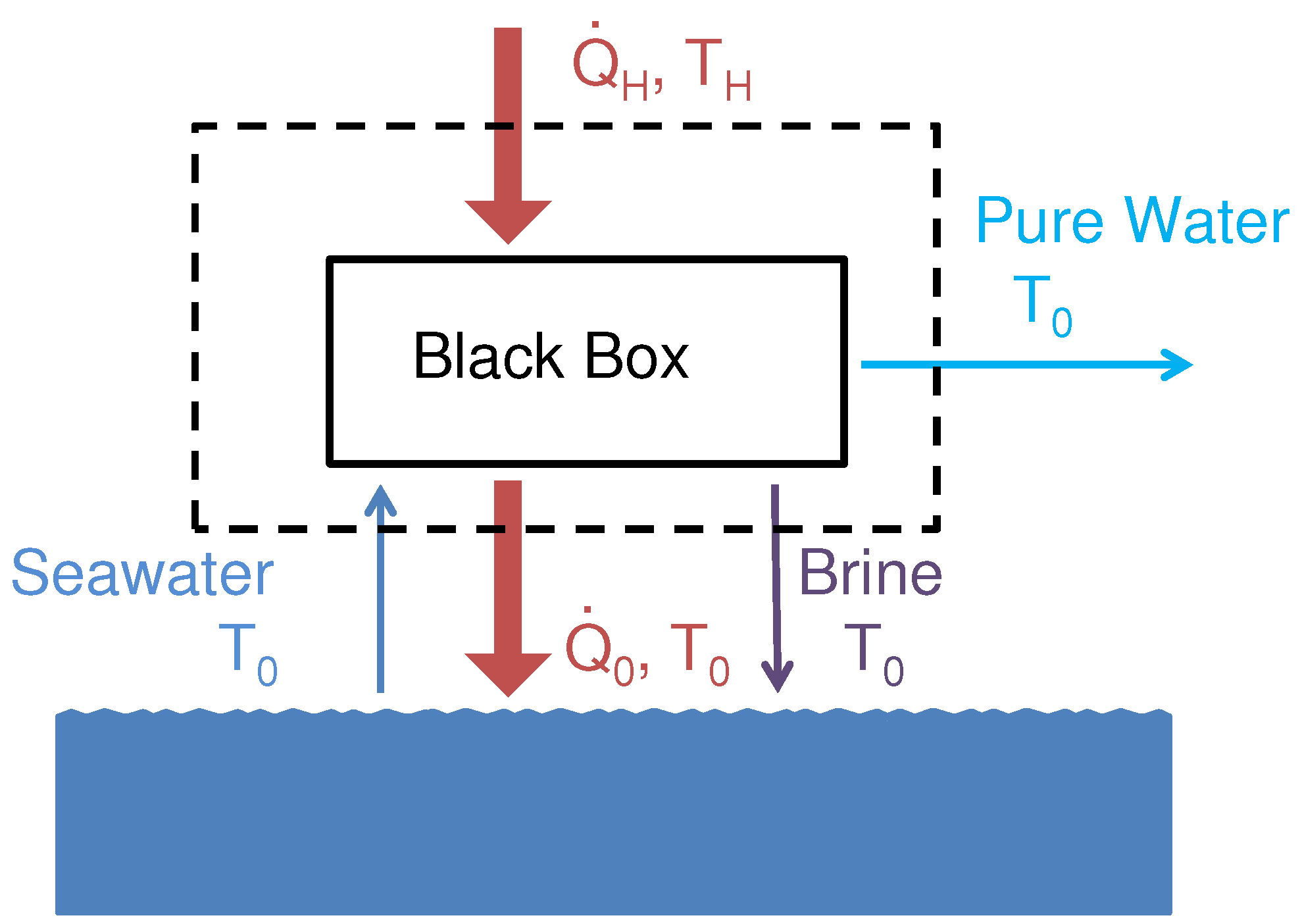
Figure 1 shows a schematic diagram of a simplified black-box desalination system with heat transfer occurring from a waste heat source at temperature,
, and to the environment at temperature,
. The control volume is selected sufficiently far from the system boundary such that all material streams (seawater, product water, and brine) are in both thermal and mechanical equilibrium with the environment (restricted dead state, or RDS).
Figure 1.
A control volume is selected around a black-box, waste heat driven desalination system such that the seawater (sw), product (p) and brine (b) streams are all at the environmental temperature, , and pressure .
Figure 1.
A control volume is selected around a black-box, waste heat driven desalination system such that the seawater (sw), product (p) and brine (b) streams are all at the environmental temperature, , and pressure .
The First and Second Law of Thermodynamics applied to the control volume in
Figure 1 are as follows:
where
,
,
h,
s, and
are the heat transfer terms from the waste heat source, heat transfer to the environment, enthalpy, entropy and mass flow rate, respectively. Equation (
1) and Equation (
2) can be combined by multiplying the Second Law by
and subtracting from the First Law:
where
g is the Gibbs Free energy, defined as
,
r is the recovery ratio, defined as
, and
is referred to as the work of separation [
16]. In the limit of reversible separation (
i.e.,
), the work of separation reduces to the least work of separation,
. Further, in the limit of infinitesimal recovery (
i.e., the recovery ratio approaches zero), the least work reduces to the minimum least work,
[
16,
18]. Using seawater properties and assuming an inlet salinity of 35 g/kg,
, the minimum least work is 2.71 kJ/kg [
19].
For waste heat driven systems, such as those considered in this study, the least heat of separation is of more interest [
16,
18]:
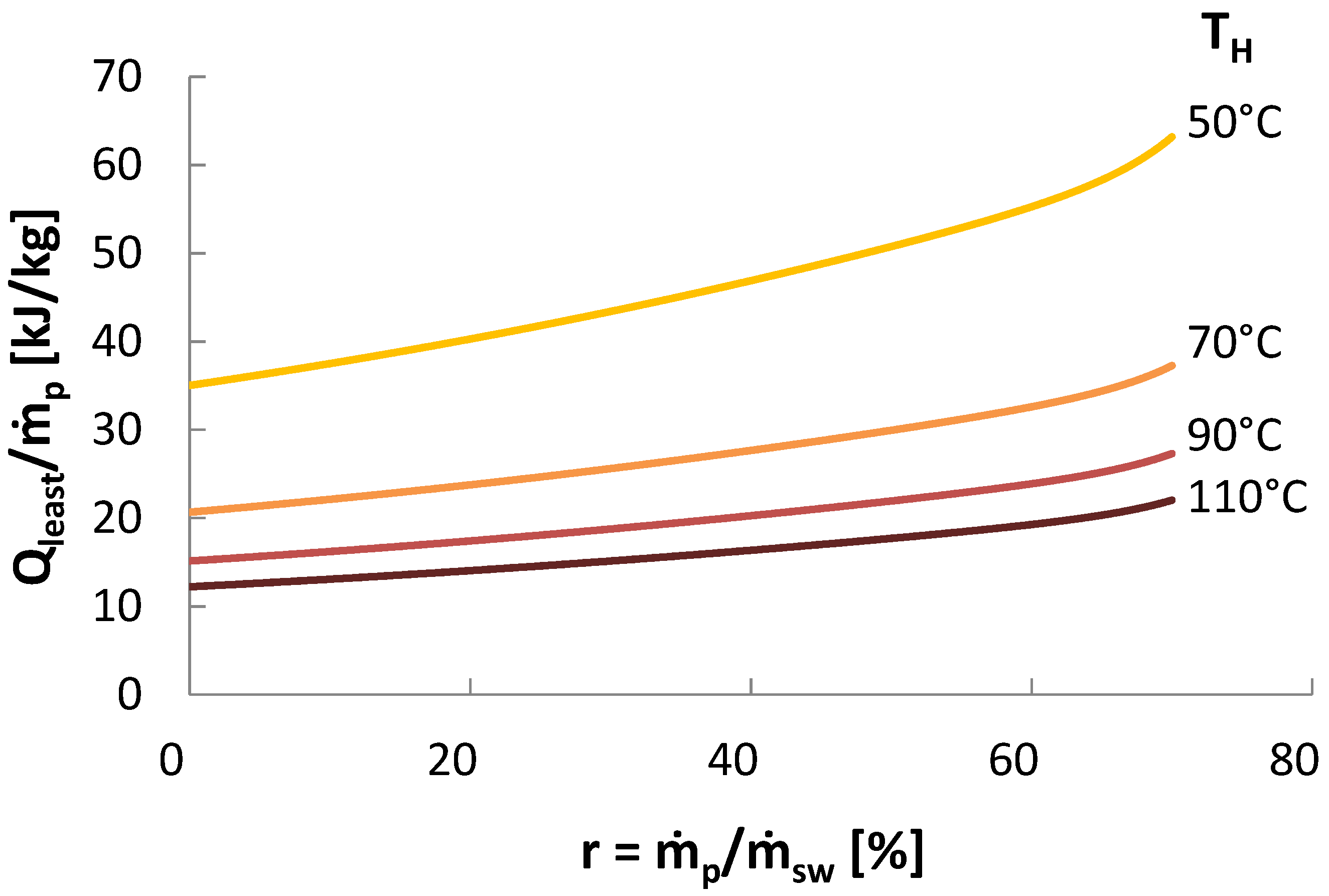
The least heat of separation is a function of both source temperature and recovery ratio, as shown in
Figure 2 [
16,
18]. In the limit of infinite source temperature, the least heat approaches the least work.
Figure 2.
Least heat of separation, is a function of recovery ratio and source temperature. Results are shown for environmental temperature of 25 .
Figure 2.
Least heat of separation, is a function of recovery ratio and source temperature. Results are shown for environmental temperature of 25 .
To compare technologies to one another, a Second Law efficiency (
) comparison is performed;
is the percent of an ideal Carnot efficiency that is achieved for each technology. This efficiency for comparing technologies is the second law efficiency, and is defined as a ratio of the minimum least exergy over the actual exergy used, as seen in Equation (
5).
The minimum least heat is defined as the minimum heat necessary to reversibly desalinate the water with near-zero recovery, where the recovery ratio is the mass flow rate of the product water divided by that of the feed. Minimum least heat is equal to minimum least work (exergy change) divided by the Carnot efficiency at the given temperatures.
Zero recovery refers to negligible concentration change of the brine caused by removing an infinitesimal amount of pure water from the feed stream. For the purpose of the process considered here (fresh water production), only the product stream, not brine stream, is the desired output. Consequently, the minimum least heat required to produce a unit of fresh water—the value at zero recovery—is the appropriate benchmark against which to compare any actual process at finite recovery. Further, it may be noted that a reversible, finite recovery process will have a Second Law efficiency below unity by the present definition.
As shown in Equation (
5), Second Law efficiency for a heat-driven desalination system is simply the ratio of the minimum least heat of separation to the actual amount of heat required for the separation process, accounting for both finite recovery ratio and irreversible processes.
Substituting Equation (
4) into Equation (
3) and renaming
as
yields:
The total entropy generation normalized to the product mass flow rate, defined here as “specific entropy generation” is represented as:
The specific entropy generation term in Equation (
6) lowers the Second Law efficiency of any real system. By analyzing specific entropy generation, one can work to improve and adapt desalination systems to minimize exergetic losses. As specific entropy generation increases, the required heat of separation also increases. Equation (
5) is plotted as a function of heat of separation for various source temperatures in
Figure 3.
Figure 3.
Second Law Efficiency for seawater desalination with an environmental temperature at 25 .
Figure 3.
Second Law Efficiency for seawater desalination with an environmental temperature at 25 .
Another commonly used efficiency parameter for thermal desalination technologies in the Gained Output Ratio (GOR), the ratio of the enthalpy of evaporation to the actual heat of separation:
Effectively, GOR measures how many times the enthalpy of evaporation is reused within a given system. Typical values for GOR range from 3 to 10, depending on the technology, operating temperatures, and other conditions. The relationship between GOR and Second Law efficiency is not simple, since the maximum GOR attainable depends on available temperatures and other conditions, while can only vary between 0 and 1.
3. Entropy Generation Mechanisms
Entropy generated through various physical processes can be calculated by using control volume analysis, where the control volume is selected such that it constrains the entirety of the process. Mistry
et al. [
16] analyzed the most common processes in desalination systems and a summary of their results is given in
Table 1.
Table 1.
Entropy Generation for Different Processes in Desalination, Partly Organized by Largest Total Contribution to the Technologies Modeled [
16].
Table 1.
Entropy Generation for Different Processes in Desalination, Partly Organized by Largest Total Contribution to the Technologies Modeled [16].
| Entropy Generation | Occurrence | Equation |
|---|
| unbalanced heat exchangers | |
| heat transfer across | |
| attainable Rankine Cycle losses | |
| heat lost to environment | |
| between output and environment | |
| flashing: evaporation from rapid pressure drop (throttling) |
|
| reverse osmosis pressure recovery |
|
| turbines | |
| throttling (valves) for fluids | |
| throttling (valves) for gases | |
| compressors, e.g., in MVC | |
| pump efficiency for fluids |
|
| salinity difference between environment and output stream | |
Temperature disequilibrium refers to the entropy generated by the exiting product and brine streams differing from ambient temperatures. Chemical disequilibrium, a result of salt concentration differences, refers to the entropy generated as the exiting saline brine mixes back in with the source seawater. The other variables and components are standard and well-known from thermodynamics. For a derivation of these equations, see Mistry
et al. [
16].
4. Unused Temperature Reduction of Waste Heat Sources
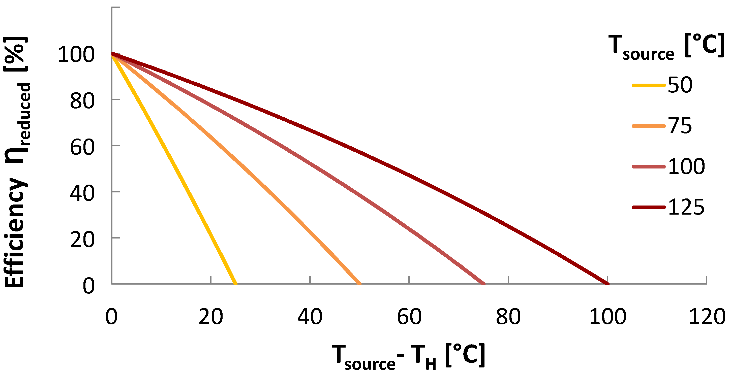
Some technologies have a maximum temperature threshold above which operation is not practical. In such systems, the source temperature may have to be reduced, resulting in significant entropy generation. It is therefore important to understand the thermodynamic losses caused by reducing the source temperature.
This becomes relevant when comparing technologies such as MED, which typically operate at 70 or below because of scaling issues, to technologies such as MSF, which may have a top temperature as high as 110–120 . To make a comparison where this temperature reduction is necessary for a fixed high temperature source, an efficiency may be used, which represents a ratio of the remaining available work divided by the original available work possible. This can be described in terms of waste heat temperatures by using , and assuming that the heat reduction occurs as a temperature gradient somewhere in the system, without losses to the environment.
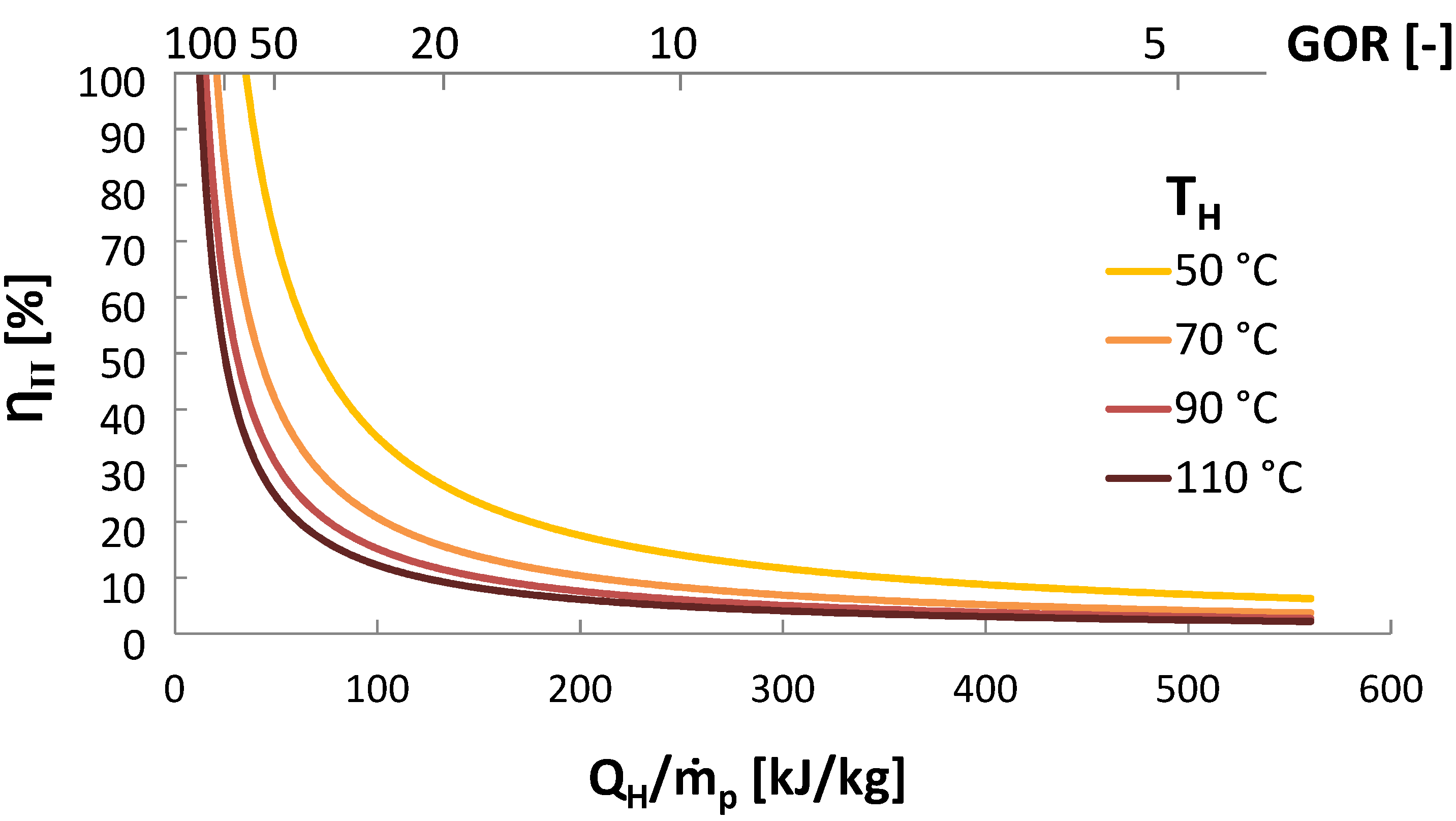
The efficiency is graphed in
Figure 4. As expected, the lower the source temperature, the greater the impact on efficiency for a reduction in temperature prior to use. Degrading the heat source prior to use results in pure exergy destruction. The severity of the loss of efficiency resulting from lowering the temperature of the waste heat prior to use illustrates the importance of matching thermal technologies to the available energy sources. These losses can be improved by using a different technology for the higher temperatures that would otherwise be left unused. For example, thermal vapor compression (TVC) is often paired with MED, since TVC can handle the high temperatures MED cannot [
20].
An example is reducing the top temperature from 90 to 70 for use in an MED system, which corresponds with an of 69%. For larger temperature differences, it is more efficient (and economical) to use another technology for the higher temperature region.
The downward curvature shows that efficiency losses accelerate as the temperature is decreased. This implies that for lower temperature thermal components such as heat exchangers, it is desirable to focus on reducing entropy generation for the colder components of a system.
Figure 4.
Efficiency factor versus temperature reduction () for various source temperatures. All results shown for environmental temperature at 25 .
Figure 4.
Efficiency factor versus temperature reduction () for various source temperatures. All results shown for environmental temperature at 25 .
5. Entropy Generation Analysis of Seawater Desalination Technologies
Entropy generation analysis for the most common seawater desalination technologies is performed in the following sections. For each technology considered, specific entropy generation is evaluated at a component level. By doing a component level analysis, it is possible to identify the largest sources of inefficiency and determine how to best improve systems.
5.1. Modeling Approximations and Assumptions
In order to make a fair comparison of the various technologies considered, operating and input conditions must be consistent for all systems. These conditions include temperatures, pressures, and salinities of the input and output streams, as well as temperature pinches and efficiencies within individual components.
Table 2 summarizes the temperatures and salinities of the input streams used in all modeling in subsequent sections. The temperatures were chosen from 50
to 110
as this represents the range from zero desalination possible (
) to where the level at which scaling usual becomes prohibitive (110
).
Table 2.
Standard input conditions used for desalination system models. Note, is only applicable to thermal technologies.
Table 2.
Standard input conditions used for desalination system models. Note, is only applicable to thermal technologies.
| Input and Output Streams for All Systems |
|---|
| 50 | | | 25 |
| 70 | | | 35 |
| 90 | | | 0 |
| 110 | | | 35 |
In addition to the standardized input conditions, the following general approximations are made:
- (1)
All processes are modeled as steady state.
- (2)
Heat transfer to the environment is negligible.
- (3)
All streams are considered well mixed and bulk physical properties are used.
- (4)
Heat transfer coefficients are constant within a given heat exchanger.
- (5)
Seawater properties can be calculated using correlations from Sharqawy
et al. [
19].
- (6)
Product water is pure (zero salinity).
- (7)
In systems with multiple stages, the number of stages was proportionally reduced for lower waste heat temperature.
- (8)
In systems with multiple stages, the recovery in each remaining stage stays roughly the same for lower temperatures.
- (9)
Pumping power may be neglected in thermal systems.
- (10)
Temperature drop across heat exchangers is between 2.5 and
Approximation 7, assuming stages must be removed to compare to different temperature sources, is crucial to comparing thermal systems driven by waste heat. In this assumption, for lower top temperatures, higher temperature stages are eliminated and the remaining stages are not changed in all ways possible, retaining their temperatures and product production rates. The rational for keeping the number of stages constant for a given temperature difference is the assumption that the components and set-points of existing real-world systems are thermally and economically optimized. The lower stages, depending on the technology, are roughly independent from the higher temperature stages, so removing higher temperature stages should have minimal effect on the subsequent stages. This approximation neglects re-optimization for the change in brine salinity, which is acceptable since the brine salinity only slightly affects thermal desalination system thermodynamics. The approximation also neglects the different flow rate of the product stream, which is acceptable, because the entropy generation in the stages and product stream components varies little between different source temperatures.
Regarding approximation 10, the temperatures differences across heat exchangers were generally thermally consistent and most were set to 3
. This condition varied slightly because of optimization: for instance, the MED model optimized the distribution of heat exchanger area between stages, while keeping the average difference within all heat exchangers at about 3
. This temperature pinch is typical of desalination industry and many past models [
16], and variation from this is small.
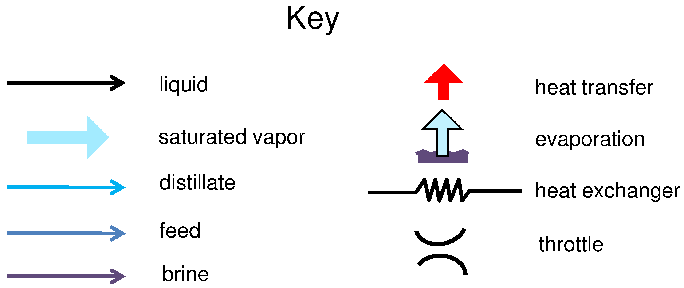
All the technologies and the specific modeling details are explained in diagrams using the symbols and colors shown in
Figure 5. In components where vapor coexists with liquid, the vapor arrows are used.
All of the modeling and calculations are done in Engineering Equation Solver (EES) [
21]. EES is a simulation equation solver that automatically identifies and groups equations that must be solved and then solves the system iteratively. The default convergence values (maximum residual <
; change of variable <
) were used in this study. Additionally, EES has built-in property packages for seawater, vapor, and air.
Figure 5.
Symbolic key for all desalination system diagrams.
Figure 5.
Symbolic key for all desalination system diagrams.
5.2. Multistage Flash
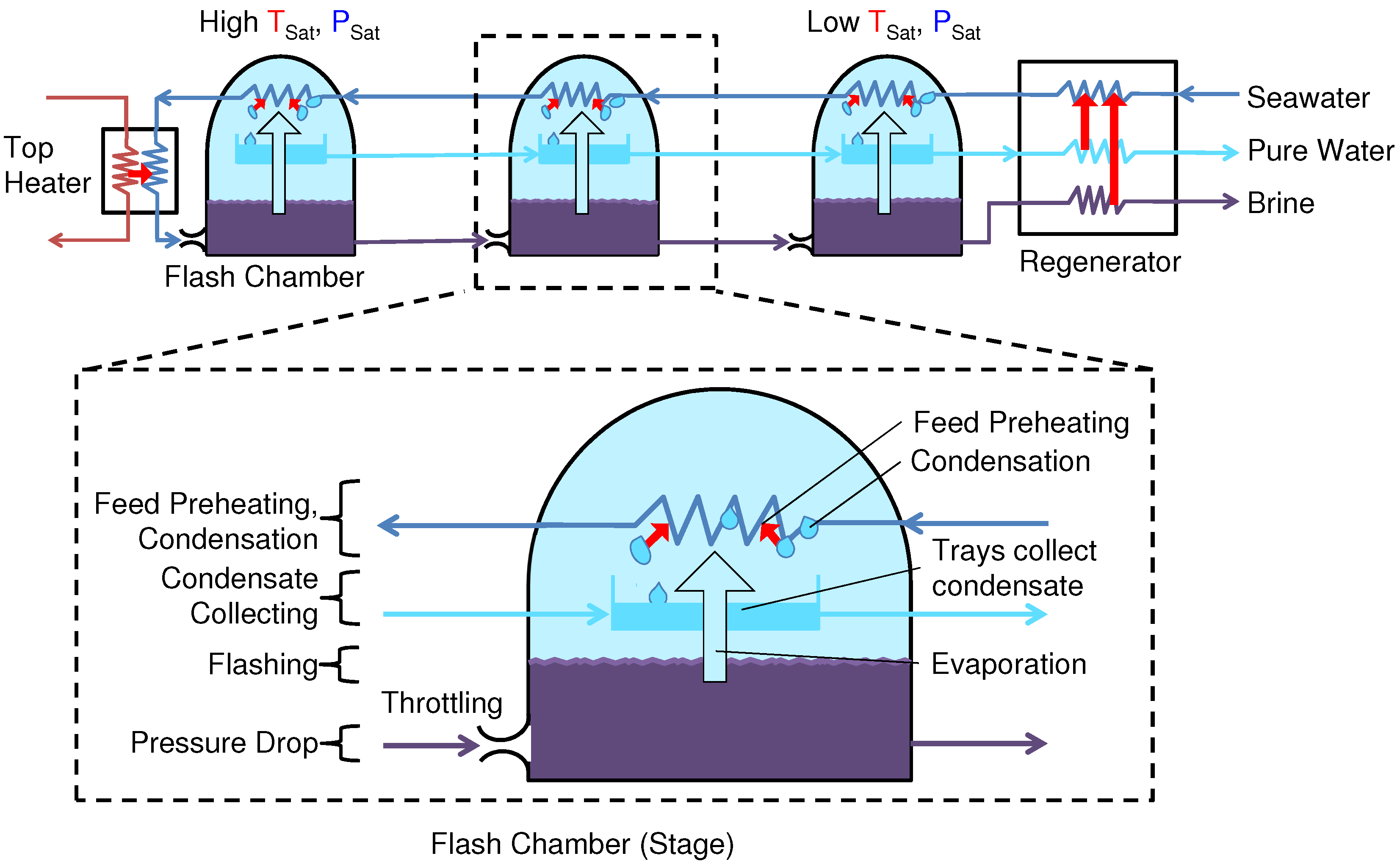
A schematic diagram of a once-through MSF system is shown in
Figure 6. A numerical model for this system was built in EES with values based upon a representative system [
9]. In MSF, seawater enters successive saturated stages, where the pressure is lower because of a throttle. This pressure drop, or flash, causes water to condense as vapor, or “flash”. To condense the vapor while preheating the feed, a counter-current heat exchanger transfers heat between this flashed water vapor and incoming seawater [
22]. A heater provides additional heat to the hot feed before the first and hottest stage, and after the coldest stage a regenerator exchanges heat between the exiting and entering streams.
Figure 6.
Flow diagram of once-through multistage flash (MSF) desalination.
Figure 6.
Flow diagram of once-through multistage flash (MSF) desalination.
A modification from typical MSF systems was the inclusion of a regenerator to exchange heat between entering and exiting streams, which was necessary to avoid large temperature gradients in the feed heaters for low top temperatures, which would have brought the GOR below 1.
The model simultaneously solves a mass and energy balance for all system components (brine and feed heaters, flashing evaporators). The inputs include recovery ratio, number of stages, and top temperatures similar to [
9], which was previously used to validate the model within 5% [
16]. The solution gives the inlet and outlet temperature, phase, salinity, and entropy generation for each part.
Several common engineering approximations were made, including those from [
9,
16]. The following approximations were not included in the universal approximation list:
Results from the present model are given in
Table 3.
Table 3.
Multistage flash modeling results.
Table 3.
Multistage flash modeling results.
| Parameter | |
|---|
| Output | | | | |
|---|
| Number of stages | n | (-) | 24 | 17 | 11 | 4 |
| Gained output ratio | GOR | (-) | 10.3 | 7.3 | 4.4 | 1.4 |
| Recovery ratio | RR | (-) | 11.1% | 7.7% | 4.3% | 1.3% |
| Steam flow rate | | (kg/s) | 0.0983 | 0.137 | 0.222 | 0.674 |
| Brine salinity | | (g/kg) | 39.4 | 37.9 | 36.6 | 35.5 |
| Second Law efficiency | | (%) | 6.28% | 5.67% | 4.98% | 3.25% |
| Entropy generation | | (J/kgK) | 182.6 | 203.2 | 233.2 | 364.5 |
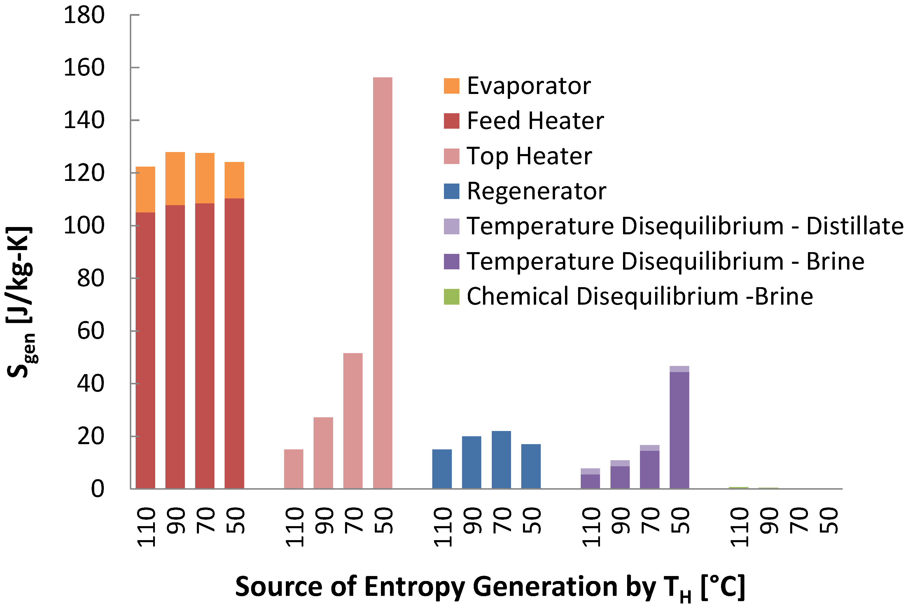
The results of entropy generation per stage show that the heating elements dominate, with the feed heater providing the largest source of entropy generation normalized by
, or
, as seen in
Figure 7 and
Figure 8. Significant entropy is generated in the temperature gradients that occur when exchanging heat between streams, and is largest for the feed heaters as this is where most of the heat exchange for the largest stream, the brine, occurs. For each stage, the entropy generation for flashing is very small: this occurs at constant temperature. At higher recovery ratios, the brine flow rate decreases, which reduces the
of the feed heaters and chemical disequilibrium of the brine. Also for higher recovery ratios, more flashing will occur in each flashing chamber and thus more entropy will be generated there.
For multistage flash, the dominant entropy generation occurred in the feed heaters, generated by heat transfer across a temperature gradient. Similarly, there was significant generation in brine heater as well as the regenerator. Temperature disequilibrium entropy generation also played a role, especially in that of the brine. In contrast, generation from chemical disequilibrium was relatively negligible. At lower temperatures, these trends changed substantially. Because the stages are left unchanged (with the high temperature stages removed and the lower temperature stages operating at the same temperatures, distillate production rates, and other conditions) there was little difference in entropy generation within stage components of the feed heater and evaporator. More simply, the stages experience nearly identical conditions between different cases, and their is associated with the distillate stream, which also changes little. This is seen in parts of the other technologies as well. Similarly, the entropy generation change in the regenerator is minimal due to minimal temperature change between cases. Since the seawater stream flow rate is much larger than the distillate stream, the seawater stream behaves like a heat reservoir at constant temperature with most of entropy generation in the distillate stream. The entropy generation from temperature disequilibrium in the distillate does not change between cases.
Figure 7.
Entropy generation per kilogram product water produced in each multistage flash (MSF) component at a heat source temperature of 110 .
Figure 7.
Entropy generation per kilogram product water produced in each multistage flash (MSF) component at a heat source temperature of 110 .
Figure 8.
Entropy generation per kilogram product water produced in each multistage flash (MSF) component for all four temperatures modeled.
Figure 8.
Entropy generation per kilogram product water produced in each multistage flash (MSF) component for all four temperatures modeled.
For the lower temperature cases, removing the high temperature stages significantly increases entropy generation in the brine stream, since the product water lost from removing stages reduces recovery, making the feed stream much larger than that of the distillate. The most substantial increase in entropy generation occurs in the brine heater, where heat transfer occurs at the top temperature. This increases substantially for lower temperature cases as well, for the above reason and because this heat transfer occurs at a lower temperature. The increase in the brine heater is so substantial as it dominates at 50 ; but it becomes minor at 110 . The from brine temperature disequilibrium becomes more important because the flow rate of seawater becomes relatively large compared to that of the distillate.
5.3. Multiple Effect Distillation
A detailed numerical model for multiple effect distillation (MED) was created by Mistry
et al. [
10], based upon more basic models in [
9,
23,
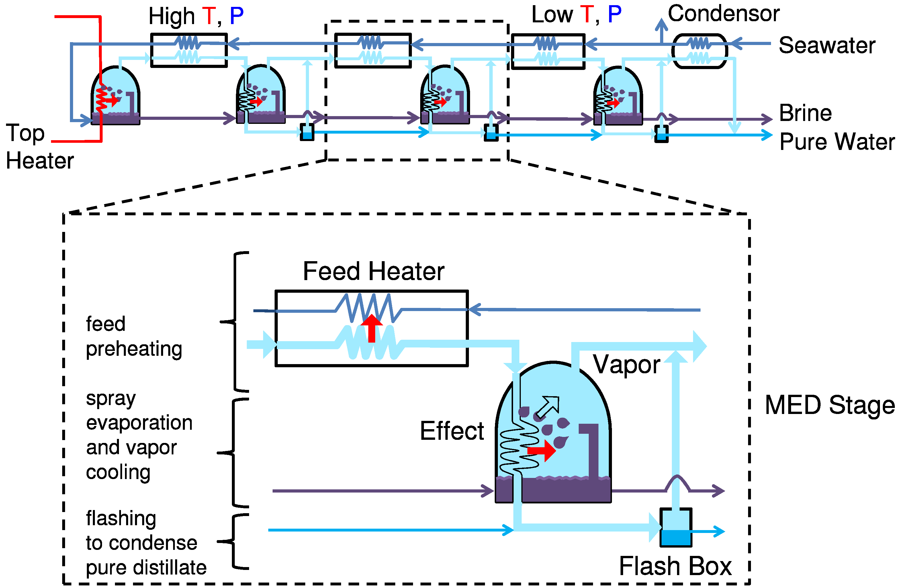
24]. A schematic diagram of a typical forward feed MED system is shown in
Figure 9.
MED shares features with MSF, including stages (called effects in MED) with generation of water vapor from seawater, and recovery of vapor latent heat to preheat the feed via a heat exchanger [
25]. However, in MED vapor passes through the subsequent (less hot) effect through a heat exchanger, and then goes through a flash box to condense pure distillate. For efficient evaporation, MED usually sprays seawater on the heat exchanger. The first effect has a steam heater to finish warming the feed, and no flash box.
Figure 9.
Flow diagram of multi-effect distillation (MED) desalination.
Figure 9.
Flow diagram of multi-effect distillation (MED) desalination.
The vapor produced in each effect is taken through a condenser where partial condensation helps preheat the incoming feed. The remaining vapor condenses while vaporizing feed from the subsequent effect. When the feed is passed from one effect to another, it is flashed.
The vapor produced in this flashing process is also added to the vapor stream in the feed preheater.
In addition to the general approximations stated above, several additional standard engineering approximations are made in this analysis:
Exchanger area in the effects is just large enough to condense vapor to saturated liquid (i.e., ) at the previous effect’s pressure.
Seawater is an incompressible liquid and the properties are only a function of temperature and salinity.
Non-equilibrium allowance (NEA) is negligible [
9].
Brine (liquid) and distillate (vapor) streams leave each effect at that effect’s temperature. Distillate vapor is slightly superheated.
The overall heat transfer coefficient in each effect, feed heater, and condenser is a function of temperature only [
9].
The MED model is created by performing component level control volume analysis coupled with modeling the heat transfer within each effect. Specifically, mass conservation, First and Second Laws, as well as heat transfer rates are evaluated in each effect, flash box, and feed heater. Properties are evaluated using IAPWS 1995 Formulation [
26]. Unlike many MED models in the literature, the model by Mistry
et al. [
10] relies on the simultaneous equation solver, EES.
For the following simulations, the temperature difference between the heat exchanger in the effects, which dominates entropy generation, varies between 2.65 and 3.3
, where the distribution of temperatures is optimized by the code, where the average is just under 3
. The terminal temperature difference between the feed heaters and condenser, which are both less important, was 5
, and was the only exception in this study to heat exchanger temperature differences being near 3
. These values were based upon a representative system [
9]. The average heat exchanger temperature difference throughout the system is about 3
, and the variation does not effect the overall conclusions of this paper. The results for both the 50 and 70
cases are summarized in
Table 4.
Table 4.
Summary of results for a forward feed multi-effect distillation system operating at 50 and 70 .
Table 4.
Summary of results for a forward feed multi-effect distillation system operating at 50 and 70 .
| Parameter | |
|---|
| Output | | | | |
|---|
| Number of stages | n | (-) | 12 | 5 |
| Gained output ratio | GOR | (-) | 9.349 | 4.048 |
| Recovery ratio | RR | [%] | 40% | 17.5% |
| Steam flow rate | | (kg/s) | 0.1119 | 0.2526 |
| Brine salinity | | (g/kg) | 58.3 | 42.4 |
| Second Law efficiency | | (%) | 10.59 | 6.58 |
| Entropy generation | | (J/kgK) | 102.4 | 139.1 |
Unsurprisingly, the MED system operating at and 12 effects is significantly more efficient (GOR of 9.3) than the system operating at with only 5 effects (GOR of 4.0). As is true of typical thermal systems, higher temperatures lead to higher thermodynamic efficiencies and therefore, higher temperature waste heat is desirable, when available. Given the large difference in GOR between the two conditions, it is clear that the total entropy generated in the case is higher. Existing MED processes are generally limited to , so higher temperature cases were excluded.
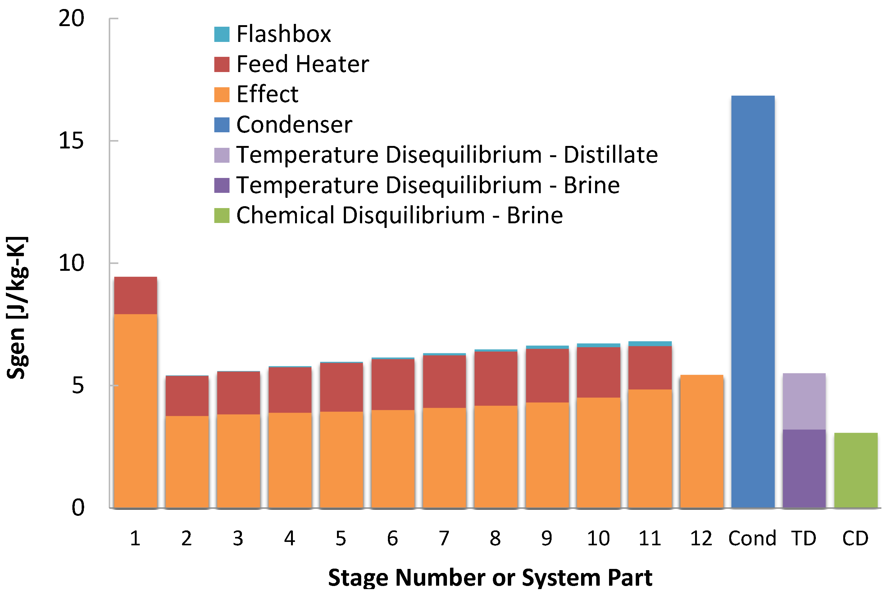
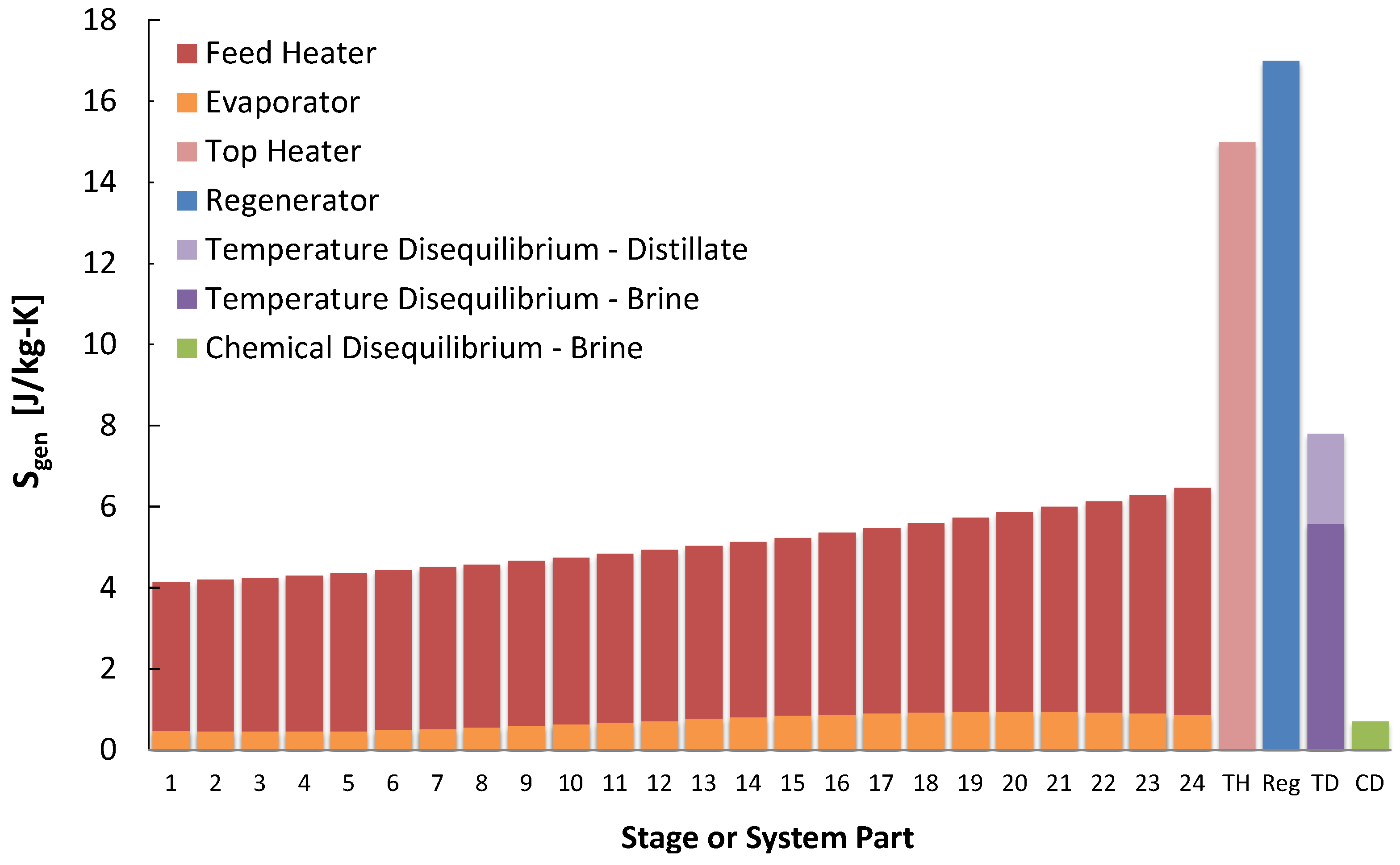
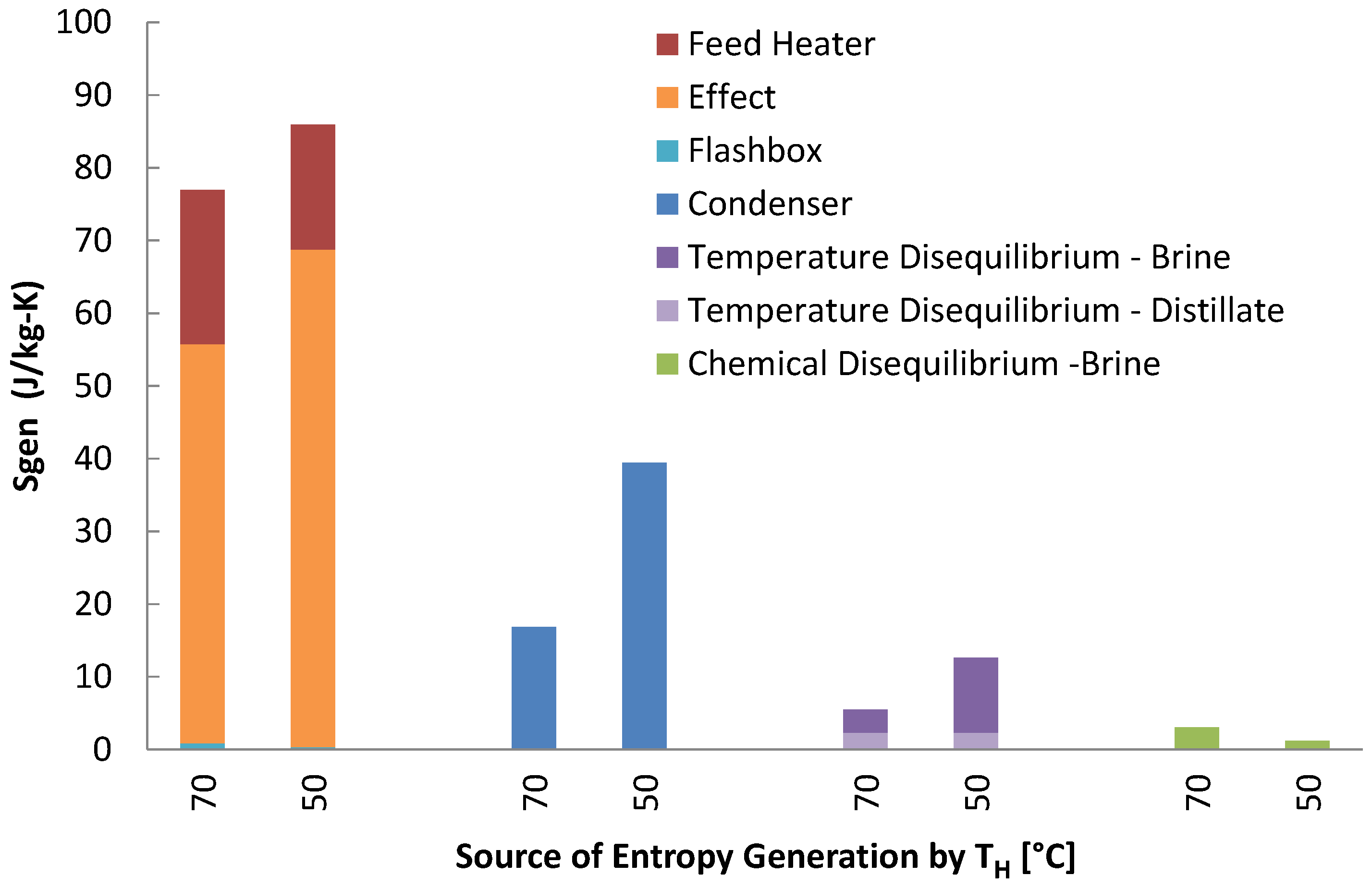
Detailed entropy generation results, by component, are illustrated in
Figure 10. From examining
Figure 10 and
Figure 11, it is clear that the condenser’s performance has the greatest impact on the overall system performance. In particular, it is the most sensitive to varying input temperature. This substantial increase of entropy generation in the condenser is due to the larger quantity of heat transfered than in individual stages, and also the relatively higher feed flow rate in the condenser, which increases entropy generation for two reasons. First, the streams have a larger average temperature difference because the condenser stream’s larger heat capacity causes it to have a lower temperature drop. Second, the average absolute temperature at which heat transfer occurs is lower in the 50
system, resulting in a higher rate of entropy generation.
Between the different temperature cases, the results are similar to that in MSF: the entropy generated in the stages changes little, while it can increase elsewhere. for the feed heater and effects did not change much for the lower temperature cases, which is a result of the stage temperatures and product water production changing little, and occurring in the distillate. The total entropy generation in the effects increases slightly, partially due to the fact that the first effect has higher entropy generation, and this addition occurs at a lower temperature.
Figure 10.
Entropy generation per kilogram product water produced in each multi-effect distillation component at a heat source temperature of 110 .
Figure 10.
Entropy generation per kilogram product water produced in each multi-effect distillation component at a heat source temperature of 110 .
Figure 11.
Entropy generation per kilogram product water produced in each multi-effect distillation component for all temperatures modeled.
Figure 11.
Entropy generation per kilogram product water produced in each multi-effect distillation component for all temperatures modeled.
Like the MSF case, the entropy generation in the system components that depend on the feed or brine flow rate increase significantly with the higher temperature states removed. As in the entirety of the paper, the entropy generation is normalized to distillate production, so the equations for entropy generation in the brine contain the ratio term . Since the volume of heated brine leaving the system has increased substantially relative to the distillate in the lower temperature case, the entropy generation from temperature disequilibrium of the brine increases. Again for the same reason of increased flow rate of the feed and brine streams, the entropy generation in the condenser increases as well. Finally, the lower recovery ratio results in lower chemical disequilibrium, although irreversibilities due to disequilibrium of the brine have a minimal effect on the overall performance of an MED system.
5.4. MSVMD
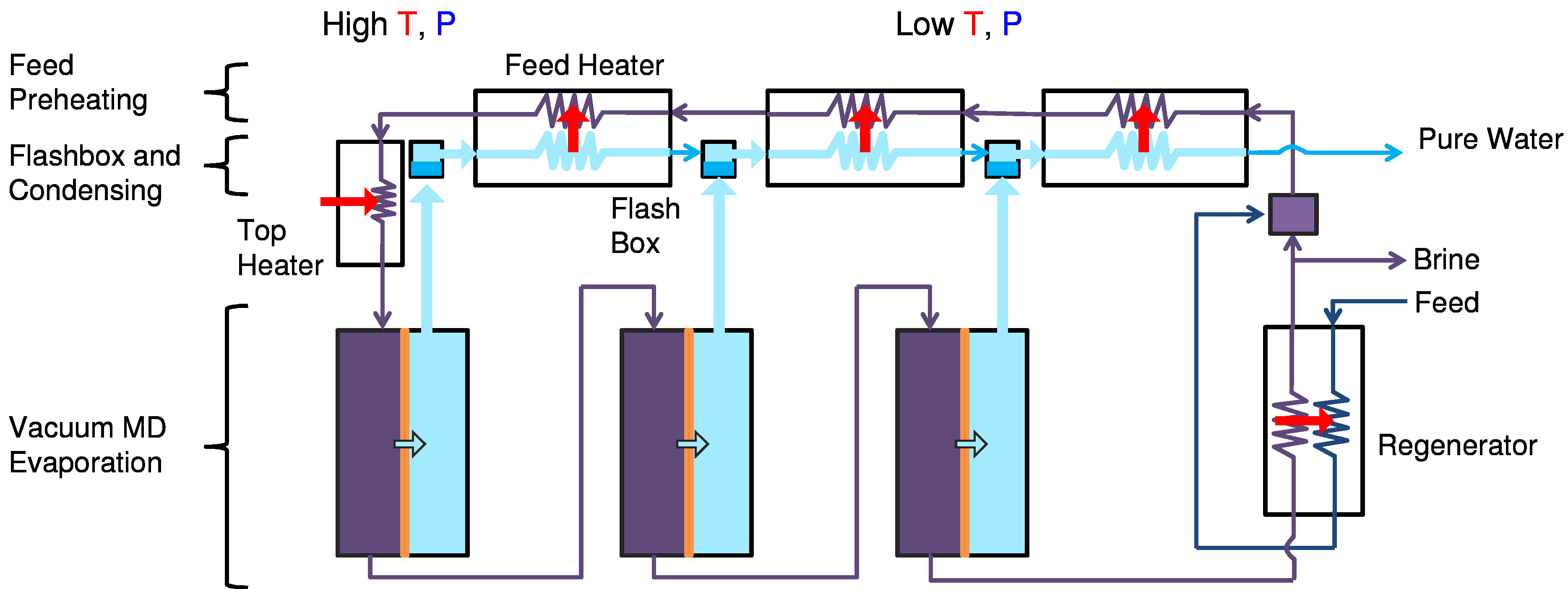
Vacuum MD (VMD) relies on a hydrophobic membrane that rejects liquid water but passes water vapor, where the water vapor passes into an evacuated chamber which is continuously emptied of vapor. The Multistage VMD (MSVMD) system used here is similar to MSF; flashing chambers are replaced by VMD modules as shown in
Figure 12. One difference is that vapor produced in each stage is slightly superheated because feed temperature near the inlet of each stage is close to previous stage’s saturation temperature. However, degree of superheat is small and extra enthalpy associated with superheat is negligible compared to latent heat of vaporization.
Figure 12.
Flow diagram of multi-stage vacuum membrane distillation (MSVMD) system.
Figure 12.
Flow diagram of multi-stage vacuum membrane distillation (MSVMD) system.
The feed stream is mixed with brine and enters a train of feed pre-heaters where it is heated by condensation energy released from water vapor. External heat input raises the feed temperature to a desired top brine temperature. The feed stream goes through stages of VMD modules which are maintained at progressively lower vacuum pressures. Some portion of brine leaving the last stage is recirculated and the rest is rejected to the environment. Pure water vapor produced from each VMD stage enters the flashing and mixing chamber where it is mixed with the product stream from previous stages. Detailed description of the system configuration and parameters can be found in [
11]. There are several assumptions made for the MSVMD model.
Heat exchanger area is just enough to fully condense the vapor; saturated liquid leaves the exchanger.
Smallest temperature difference between any heat exchanging streams are set to be 3 .
Heat transfer coefficient and mass transfer coefficient are calculated using pure water properties.
Each stage of VMD module is discretized into computational cells in order to be solved by finite difference method developed by Summers
et al. [
27].
The energy, entropy, and mass balance equations are solved in each computation cell. Vapor flux,
J, is calculated as:
where
is the saturation pressure of the feed stream at the membrane surface,
is the vacuum pressure on the product water side, and
B is membrane distillation coefficient that is calculated using Knudsen and viscous flow models [
28]. Interested readers are referred to Summers
et al. [
27] for more detail on the finite difference model for MD.
Simulation results are summarized in
Table 5.
Table 5.
Multistage Vacuum Membrane Distillation (MSVMD) Results.
Table 5.
Multistage Vacuum Membrane Distillation (MSVMD) Results.
| Parameter | |
|---|
| Output | | | | | |
|---|
| Number of stages | n | [-] | 18 | 11 | 4 |
| Gained output ratio | GOR | [-] | 7.8 | 4.8 | 1.8 |
| Recovery ratio | RR | [%] | 8.48 | 5.25 | 1.97 |
| Second Law efficiency | | [%] | 4.84 | 4.05 | 2.57 |
| Entropy generation | | [J/kgK] | 178.7 | 215.5 | 344.1 |
Just as other thermal systems have higher efficiency when the steam temperature is higher, MSVMD shows drastic improvement: GOR more than quadruples as the steam temperature increases from 50
to 90
. Like GOR, the Second Law efficiency increases with steam temperature. Component-wise analysis of entropy generation for the steam temperature of 90
is shown in
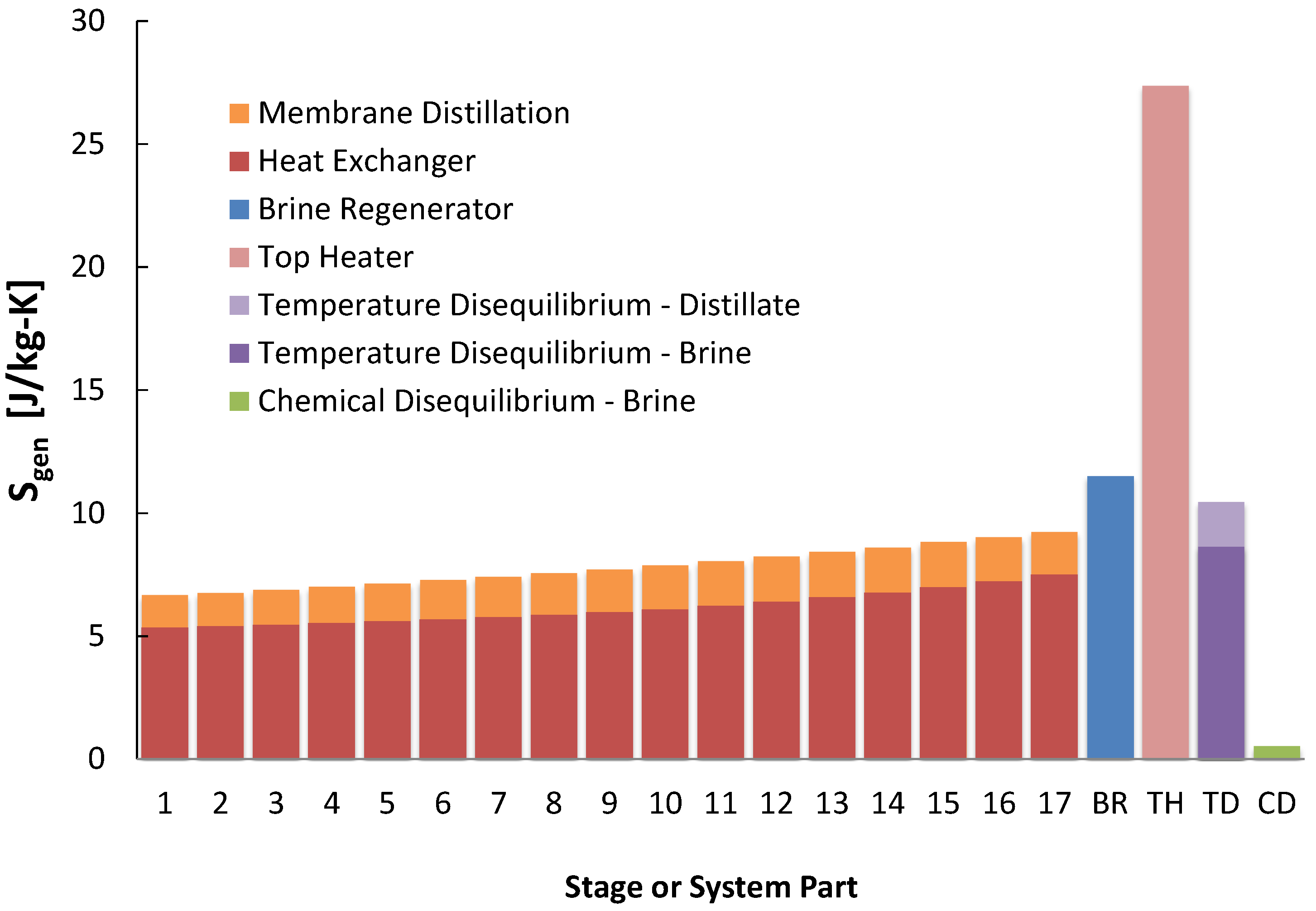
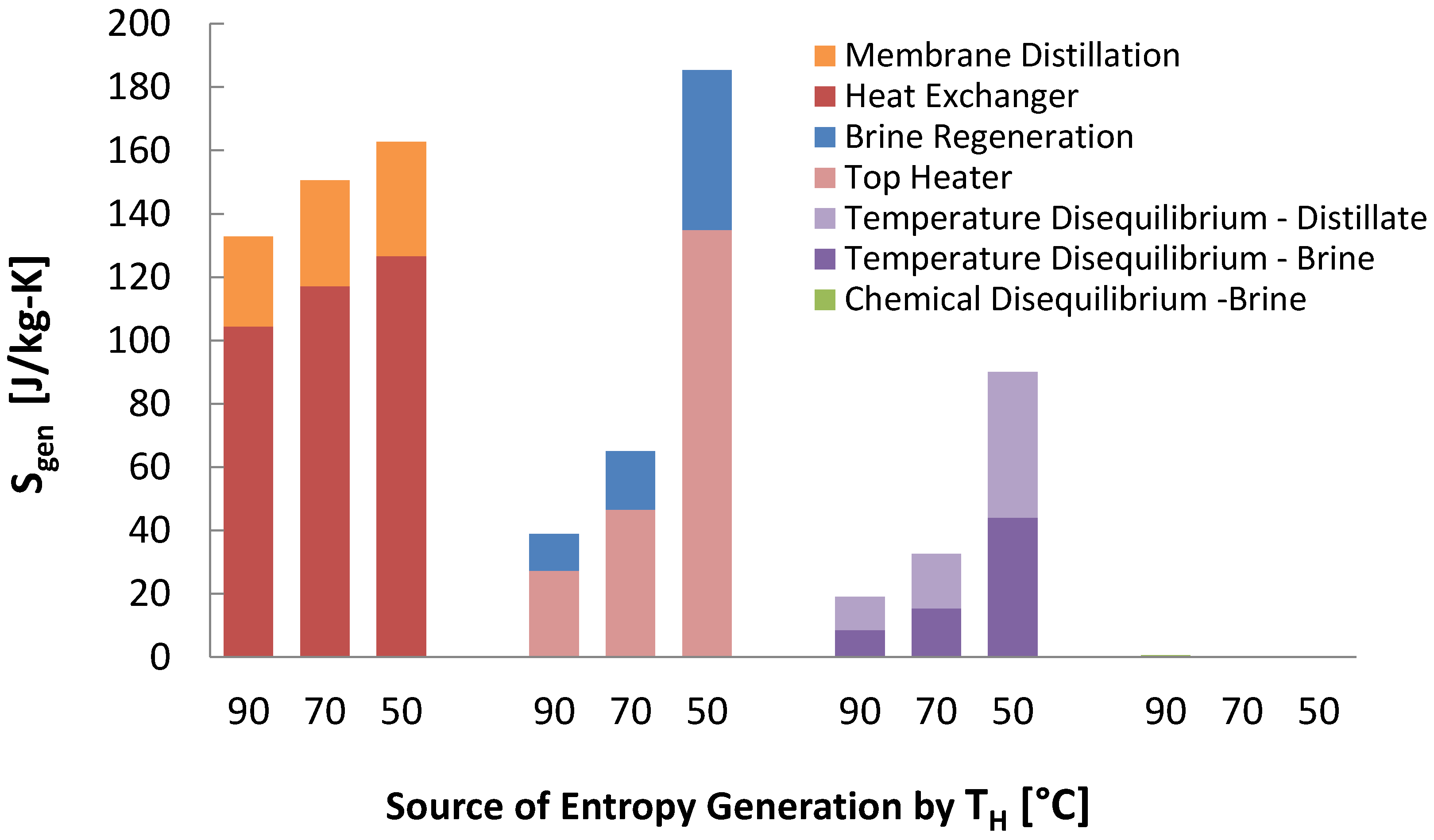
Figure 13. The more general component entropy generation analysis with all three temperatures tested is shown in
Figure 14.
The biggest contribution of specific entropy generation is due to heat exchangers in the MSVMD stages. The other heaters temperature disequilibrium is highest for 50 case for both brine and distillate. Total entropy generation is higher for the 50 for all components except chemical disequilibrium. Chemical disequilibrium is larger for higher steam temperatures because the recovery ratio is higher, which creates a larger difference between the least heat and minimum least heat of separation. However, chemical disequilibrium is negligible compared to other terms. Another major contribution is the top heater, especially for the 50 case. This occurs because the energy regeneration is so low that significantly more energy has to be transferred to the feed stream from the top heater, generating large amount of entropy, and because the heat transfer occurs at lower temperature. It should be noted that the absolute amount of entropy generation in each case do not differ by a lot. It is the low permeate production rate that significantly raises the specific entropy generation in each of the categories. In thermodynamic perspective, the main drawback of using low temperature waste steam is a low recovery ratio, resulting in high specific entropy generation.
Figure 13.
Entropy generation per kilogram product water produced for each component in multistage vacuum membrane distillation (MSVMD) for a heat source temperature of 90 .
Figure 13.
Entropy generation per kilogram product water produced for each component in multistage vacuum membrane distillation (MSVMD) for a heat source temperature of 90 .
Figure 14.
Entropy generation per kilogram product water produced for each component in multistage vacuum membrane distillation (MSVMD) for all 3 temperatures modeled.
Figure 14.
Entropy generation per kilogram product water produced for each component in multistage vacuum membrane distillation (MSVMD) for all 3 temperatures modeled.
5.5. Humidification-Dehumidification
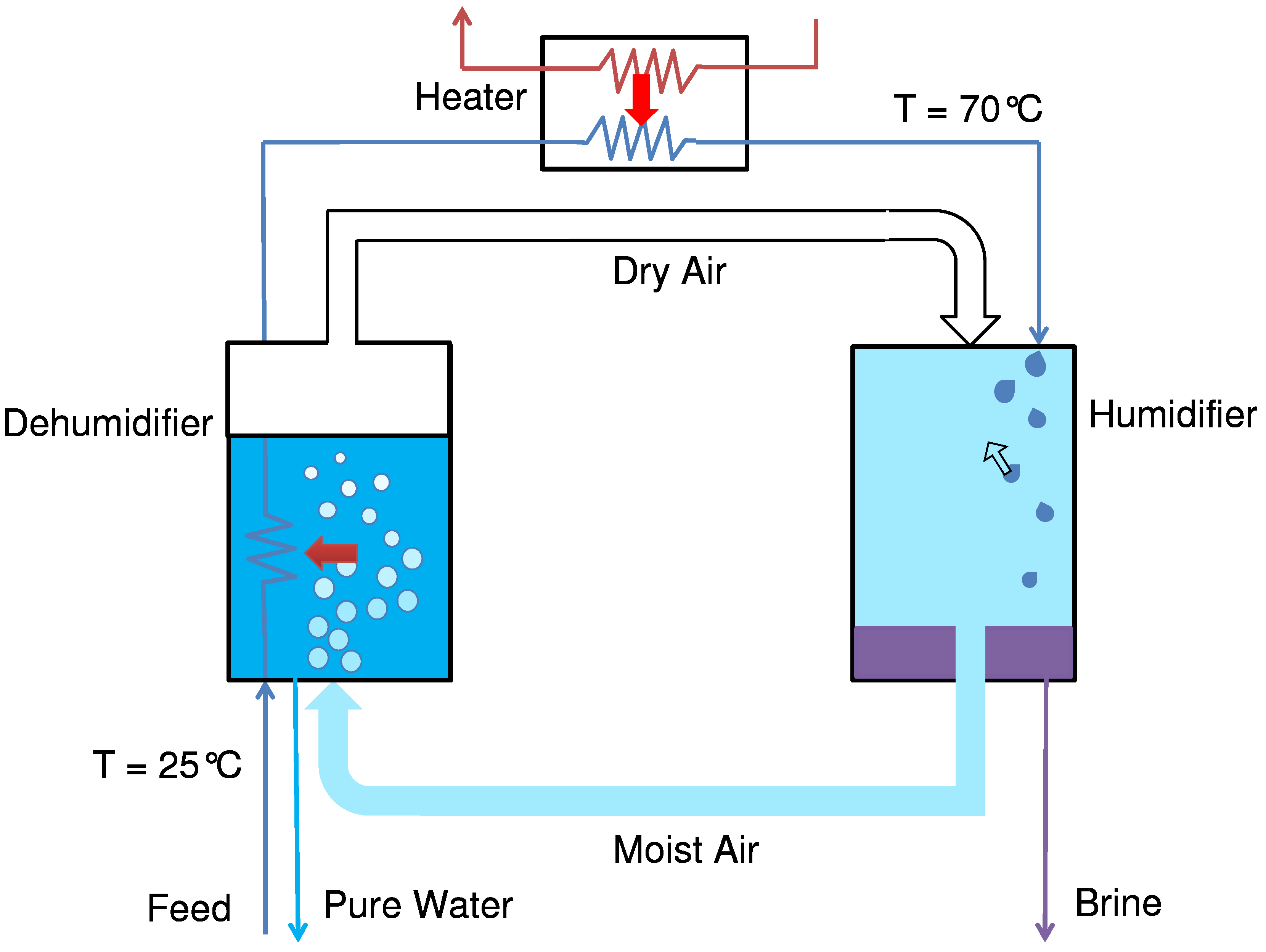
Humidification-dehumidification desalination, inspired by the natural rain cycle, consists of a humidifier, heater, and dehumidifier. A closed air open water (CAOW) HDH configuration is depicted in
Figure 15. Feed water enters the system at ambient temperature and is pre-heated by hot moist air condensing in a bubble-column dehumidifier. The feed is then heated to a desired top temperature using an external heat source, in this case, a waste heat source. Subsequently, the feed water moves in to the humidifier where it is brought in direct contact with cold dry air, typically as a spray. The feed gets concentrated as it loses its water content to the cold dry air which in turn gets humidified and heated up. The hot moist air then condenses in the dehumidifier to give pure product water.
Figure 15.
A flow path diagram of humidification-dehumidification (HDH) desalination.
Figure 15.
A flow path diagram of humidification-dehumidification (HDH) desalination.
To simulate the HDH process, a numerical EES model developed by Mistry
et al. [
12] was used after modification to include a graphical temperature pinch analysis [
29]. The inputs used in modeling are given in
Table 6. A temperature pinch (
) of 3 K between the moist air and water streams was maintained in both the dehumidifier and the humidifier. The Heat Capacity Ratio, defined as the ratio of the maximum possible enthalpy change of the cold stream to that of the hot stream, in the dehumidifier (
) was set to be 1 for balancing the dehumidifier, reducing entropy generation and optimizing the GOR of the system [
30,
32]. The moist air was assumed to be saturated. The HDH process was simulated for three different system top temperatures:
= 50
, 70
and 90
. The results are shown in
Table 7.
Table 6.
Input for a humidification-dehumidification desalination system.
Table 6.
Input for a humidification-dehumidification desalination system.
| Parameter | | | |
|---|
| Input | Symbol | Units | Value |
| Temperature pinch | | () | 3 |
| Dehumidifier Heat Capacity Ratio | | (-) | 1 |
| Moist Air Relative Humidity | | (%) | 100 |
Table 7.
Summary of results for a Humidification-dehumidification system operating at 50, 70 and 90 .
Table 7.
Summary of results for a Humidification-dehumidification system operating at 50, 70 and 90 .
| Parameter | | | | | |
|---|
| Output | Symbol | Units | | | |
|---|
| Gained output ratio | GOR | (-) | 2.1 | 2.2 | 1.7 |
| Recovery ratio | RR | (%) | 7.1 | 4.8 | 2.4 |
| Heat input | | (kJ/kg) | 1173 | 1118 | 1405 |
| Water-air mass flow rate ratio | MR | (-) | 4.1 | 2.5 | 1.6 |
| Brine salinity | | (g/kg) | 37.7 | 36.8 | 35.8 |
| Entropy generation | | (J/kgK) | 564 | 414 | 325 |
| Second Law efficiency | | (%) | 1.29 | 1.85 | 2.49 |
With increasing top temperature, the recovery ratio steadily increased. However, unlike MED and MSF, in HDH, the entropy generated per product water increased with top temperature, an observation that was also noted previously by Narayan
et al. [
30]. GOR on the other hand increased with temperature and then decreased. This changing trend occurs because an increase in top temperature leads to both an increased permeate production for a given feed flow rate and increased
.
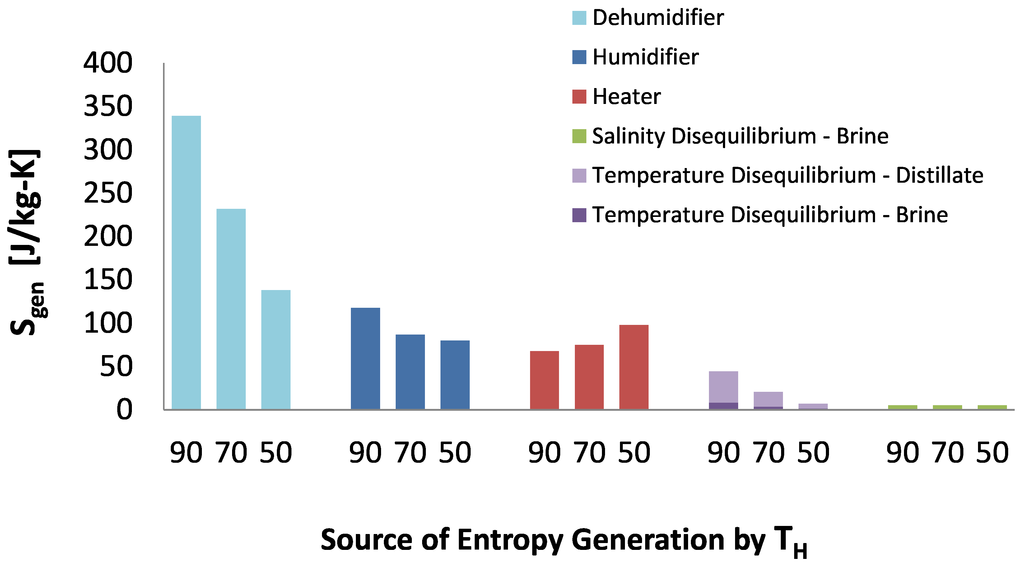
A breakdown of entropy generation with temperature is given in
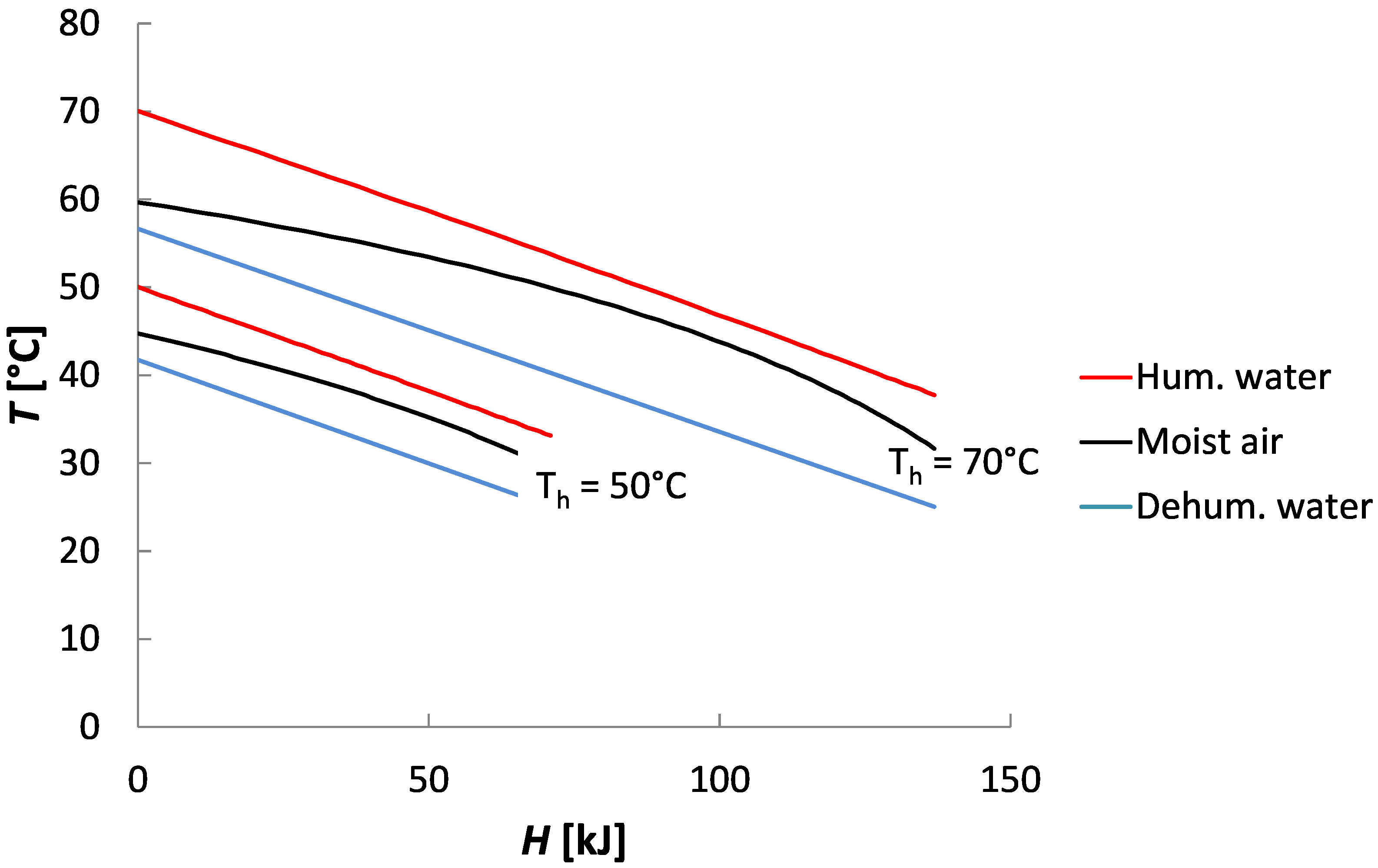
Figure 16. Most of the entropy generation happened in the dehumidifier and in both the humidifier and the dehumidifier, the entropy generated increased with an increase in top temperature. This arises because the specific heat capacity of saturated air is nonlinear with temperature causing large temperature gradients in the heat exchangers in both components. The effect is clearly visible in the temperature-enthalpy profiles shown in
Figure 17. While the minimum temperature pinches are the same at 50
and 90
, the nonlinear specific heat capacity of moist air, causes the average temperature difference between moist and water to increase with increasing top temperature. This also causes the average temperature difference between moist air and water in the dehumidifier to be higher than that in the humidifier. The larger average temperature difference directly causes more entropy to be generated during heat transfer. Entropy generation during condensation in the presence of noncondensable gases has been studied in detail by Thiel and Lienhard [
31].
Performance at higher top temperatures can be however improved very substantially by using extractions of moist air from the humidifier to the dehumidifier to allow the water streams to better match the temperature of the moist air streams [
33]. An extraction is simply removing some of the flow, typically the vapor and air mixture, to modify the
so that the enthalpies are better balanced, allowing for a smaller temperature difference when exchanging heat. For HDH systems which do not use extractions, the system is most efficient at lower top temperatures between 50
and 70
for inlet conditions considered here.
Figure 16.
Entropy generation per kilogram product water produced in each humidification-dehumidification component for all 3 temperatures modeled.
Figure 16.
Entropy generation per kilogram product water produced in each humidification-dehumidification component for all 3 temperatures modeled.
Figure 17.
Temperature-enthalpy profiles for water and moist air streams in Humidification Dehumidification Desalination. The dehumidifier and humidifier T-H curves for = 50 and 90 are shown. The minimum temperature pinch is set between cases. The larger curvature in the 70 case increased the average temperature gradient for heat exchange, and is the reason humidification-dehumidification (HDH) efficiency decreases at higher temperature, unlike other technologies.
5.6. Organic Rankine Cycle
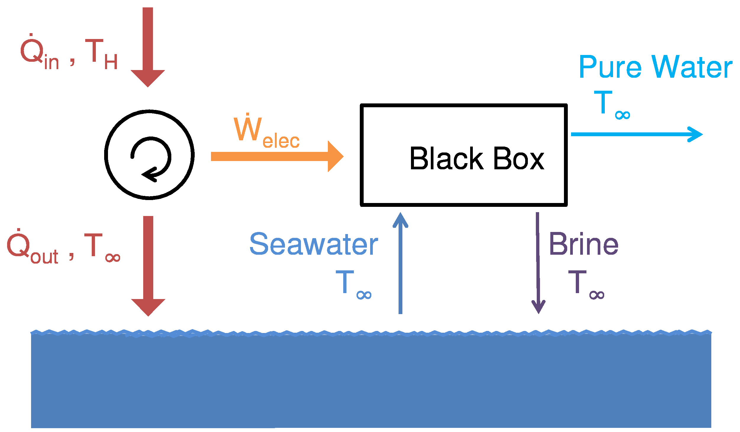
In terms of thermodynamics, electric energy has higher quality than thermal energy (e.g., waste heat) because heat cannot be continuously converted into work with 100% efficiency. Therefore, for electrically driven desalination technologies to be compared in a fair way with waste heat, heat input that would have produced the electrical work should be considered. This is done by adding a cycle to convert heat input into work, which results in a modified version of the blackbox diagram (
Figure 1) to include this step:
Figure 18.
A holistic analysis and literature review was done on the available technologies that use low temperature waste heat as a heat source, including Organic Rankine Cycles (ORCs), thermoelectrics, Stirling engines, and other cycles. The literature consistently found that the most efficient and most technologically feasible technology for temperatures between 50 and 110
was ORCs [
7,
34,
35,
36,
37].
Figure 18.
Blackbox diagram for powering electric desalination systems with waste heat.
Figure 18.
Blackbox diagram for powering electric desalination systems with waste heat.
The Rankine cycle in some form is perhaps the most used thermodynamic cycle in the power industry, and are used with nuclear and fossil fuels alike. The Rankine cycle operates within the vapor dome of the working fluid, with both heating and heat rejection resulting in phase change at constant pressure and temperature [
38]. Work is produced by a turbine operating near the saturated vapor region, and work input, in the form of pumping, is required for pressurization in the liquid or saturated liquid region.
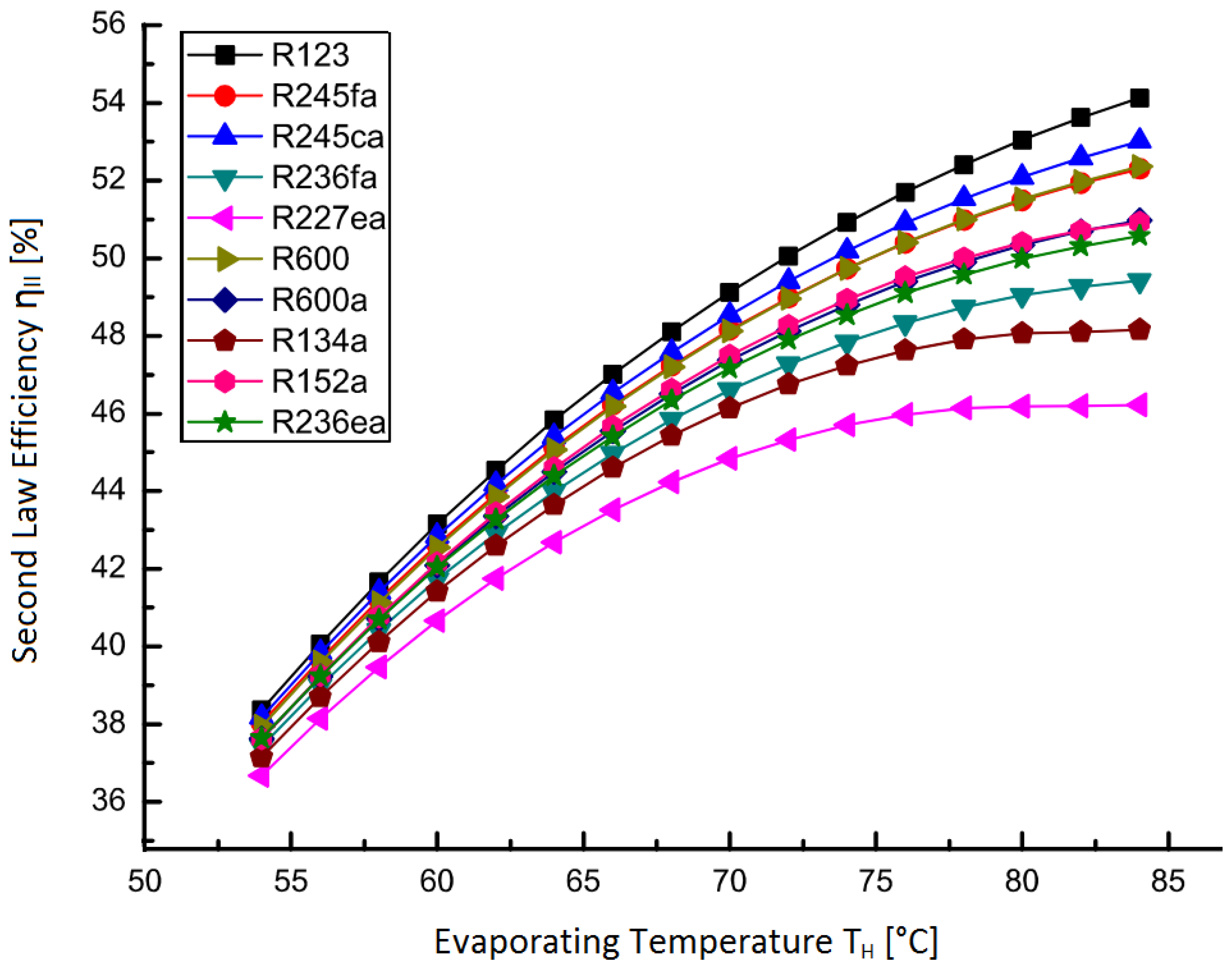
ORCs use an organic compound for the working fluid, instead of water, due to a higher vapor pressure at lower temperature. A variety of cycle improvements may be implemented, including superheat, reheat, and regeneration, but the very low temperatures under study led to the conclusion that a standard Rankine cycle was suitable. The best performing working fluid, R123, was taken from a review on Rankine cycle compounds [
13], with efficiencies from that study (
Figure 19).
The Second Law efficiency from this data was used in calculating the overall performance of the electrical desalination technologies operating on waste heat. The organic compounds have similar performance curves, so the working fluid chosen does not make a large difference. This data was readily adaptable to the present study since the inlet temperature for this data roughly matches that of the thermal cycle modeling above (25 vs. 26 ). A line of best fit was used for temperatures just outside this range (<7 ).
Figure 19.
Organic Rankine cycle Second Law efficiency
vs. evaporating temperature with
from Shengjun
et al. [
13].
Figure 19.
Organic Rankine cycle Second Law efficiency
vs. evaporating temperature with
from Shengjun
et al. [
13].
The entropy generation per unit product from using a Rankine cycle can be calculated from the definition of
in terms of work, Equation (
5), and the relation between
and
, as seen in Equation (
6):
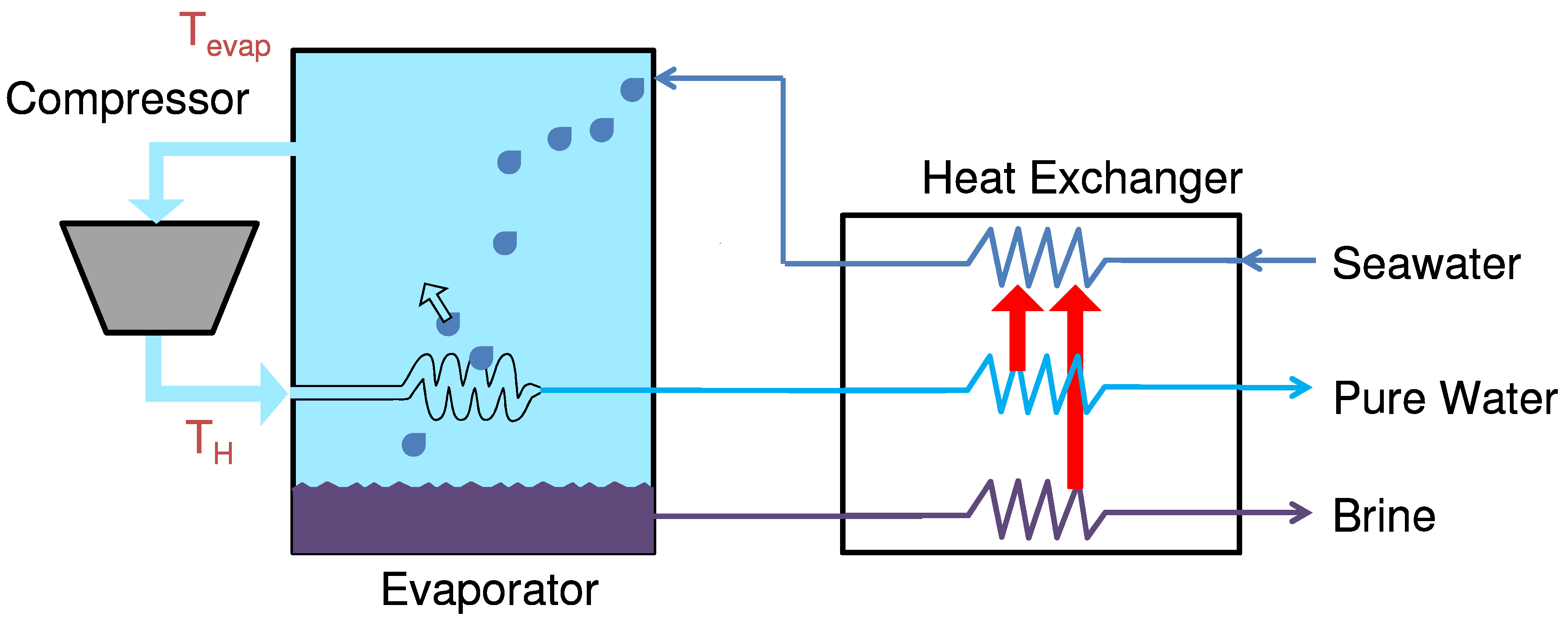
5.7. Mechanical Vapor Compression
Mechanical vapor compression (MVC) is a desalination technology that uses a compressor to pressurize and heat water vapor, then condenses this vapor into pure distillate using a heat exchanger with the incoming seawater. As seen in the schematic diagram in
Figure 20, seawater enters the system and is preheated by the exiting pure water and brine streams. The preheated seawater is then partially evaporated by spraying onto the hot evaporator heat exchanger. This water vapor exits into the compressor, where the adiabatic pressurization causes it to heat up. This vapor then goes inside the evaporator heat exchanger that helped evaporate it in the first place, but now gives off heat, causing it to cool and condense out pure distillate.
A numerical EES model was created which simultaneously solved the equations for energy and mass balances for a single stage mechanical vapor compressor desalination system. The results of this model previously appeared in prior work by Mistry
et al. [
15].
Figure 20.
Single effect mechanical vapor compression process (MVC) with spray evaporation.
Figure 20.
Single effect mechanical vapor compression process (MVC) with spray evaporation.
System operating conditions used in [
39,
40] were used in this study (
Table 8).
Table 8.
Mechanical vapor compression (MVC) design inputs.
Table 8.
Mechanical vapor compression (MVC) design inputs.
| Input | Symbol | Value |
|---|
| Top brine temperature | | 60 |
| Pinch: evaporator-condenser | | |
| Pinch: regenerator | | 3 |
| Compressor inlet pressure | | 19.4 kPa |
| Recovery ratio | RR | 40% |
| Isentropic compressor efficiency | | 70% |
The smaller pinch in the evaporator-condenser is due to the high heat transfer coefficients found with phase change compared with conventional flow. The model outputs are presented in
Table 9 and the entropy generation between different MVC components is presented in
Figure 21.
Table 9.
Mechanical vapor compression model outputs.
Table 9.
Mechanical vapor compression model outputs.
| Output | Symbol | Value |
|---|
| Specific electricity consumption | | 8.84 kWh/m3 |
| Discharged brine temperature | | 27.2 |
| Product water temperature | | 29.7 |
| Compression ratio | | 1.15 |
| Second Law efficiency | | 8.5% |
Figure 21.
Entropy generation per kilogram product water produced in each mechanical vapor compression component for all three temperatures modeled.
Figure 21.
Entropy generation per kilogram product water produced in each mechanical vapor compression component for all three temperatures modeled.
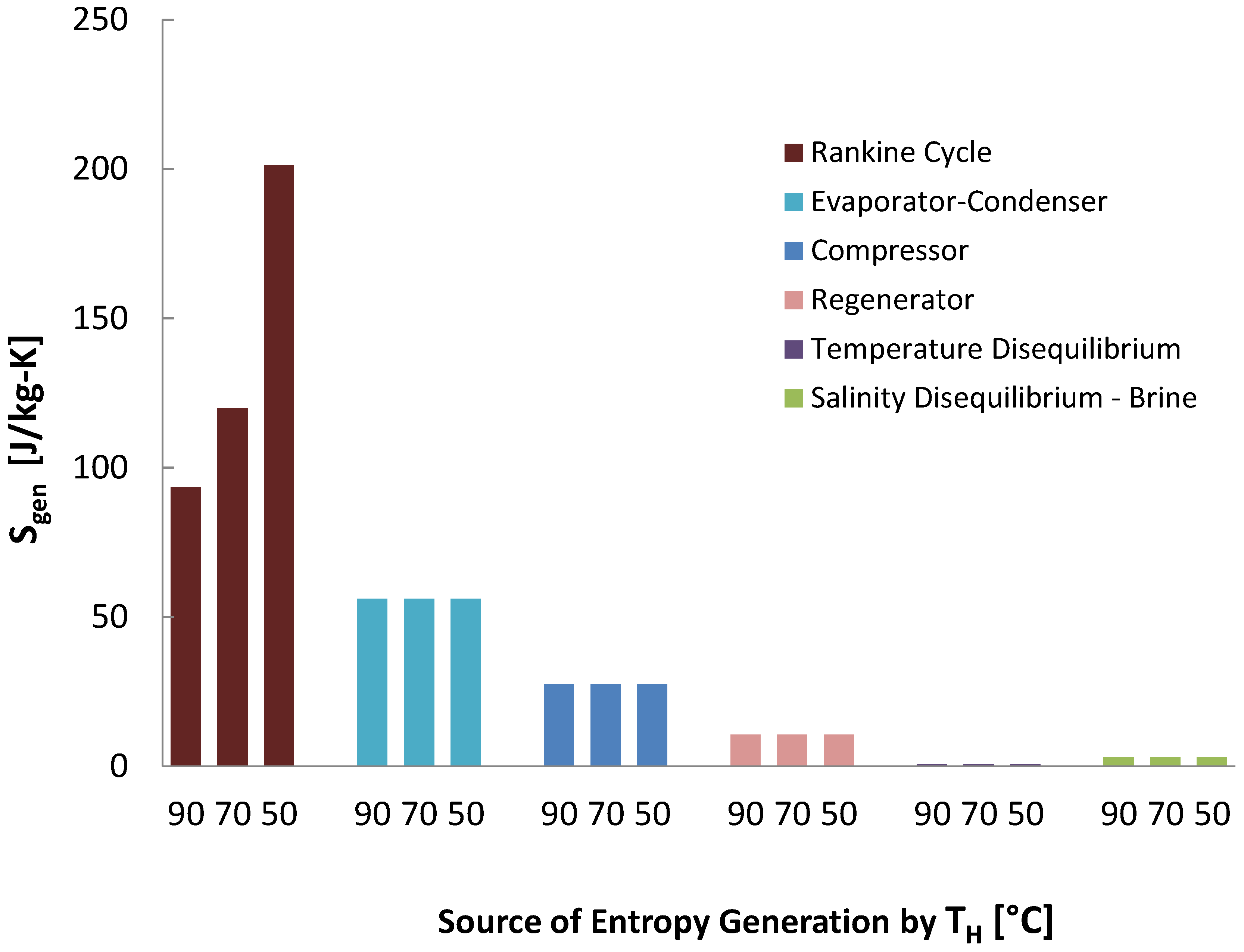
The Rankine cycle for converting a heat input to electrical work was the dominant source of entropy generation. The ORC was also the only component of the system whose
differed when operated at different temperature, with performance declining as the heat source temperature reduced. This performance decline is typical of any power cycle. This
variation only with the ORC means that the design of MVC systems need not differ for waste heat applications, provided using a power cycle to convert heat input to electrical work is feasible for a particular project. The evaporator-condenser dominated entropy generation in MVC itself, as most heat transfer within the system occurs in this part. This inefficiency increases the required compression ratio and related work. It can be improved by reducing the temperature gradients in evaporation and condensation, e.g., by increasing condensation heat transfer coefficients [
41] or increasing surface area [
42]. The vapor compressor itself was the next largest source of entropy generation; more efficient air compression technologies may significantly improve MVC efficiency. Entropy generation from temperature gradients in the regenerator was the next largest source of entropy generation; the roughly equal incoming and outgoing heat capacity (
=
+
) means the system is balanced, reducing temperature divergence in the heat exchange. The higher recovery ratio and overall good efficiency led to a relatively large role of entropy generation from chemical disequilibrium. As this is a simple one stage MVC system, and since much of the entropy generation is in a mechanical component, the compressor, and in two phase heat transfer, significant gains in efficiency can be made with superior designs, such as multistage systems [
43] and various technologies. It is worth noting that the assumptions for the MVC cycle here are less conservative than those of the other technologies, with smaller temperature differences in the heat exchangers.
Since the system is powered by electricity produced by the Rankine cycle, the operation of MVC itself is unaffected by the use of waste heat, and the component entropy generation remains identical between the different temperature cases. Like many other cycles, the Rankine cycle gets less efficient with lower temperature differences, causing worse performance at lower temperatures. The entropy generation in ORC dominates in MVC, so its performance worsens notably with lower temperature waste heat sources.
5.8. Reverse Osmosis
Reverse osmosis is globally the dominant seawater desalination technology, and relies on high pressures to overcome osmotic pressure to force water through a membrane that rejects the salts. Unlike the thermal technologies, reverse osmosis is so efficient and near the theoretical least work (typically 2–3 times ) that temperature changes in the water are negligible, and the entropy generation study therefore focuses on pumping. This differs significantly from the previous systems, where thermal effects dominated and pumping effects were negligible, and can be observed with the equation for from temperature disequilibrium.
A simple single stage RO system was modeled which incorporated pressure recovery from the brine. This standard system design was created with design and values from ERI, using their pressure exchanger [
14], and was used previously by some of the authors [
16]. The inputs are given in
Table 10.
Table 10.
Reverse Osmosis (RO) System Input Parameters.
Table 10.
Reverse Osmosis (RO) System Input Parameters.
| Input | Symbol | Value |
|---|
| Pump efficiency | | 85% |
| Pressure exchanger efficiency | | 96% |
| Feed pressure | | 2 bar |
| RO pressure | | 69 bar |
| Recovery ratio | RR | 40% |
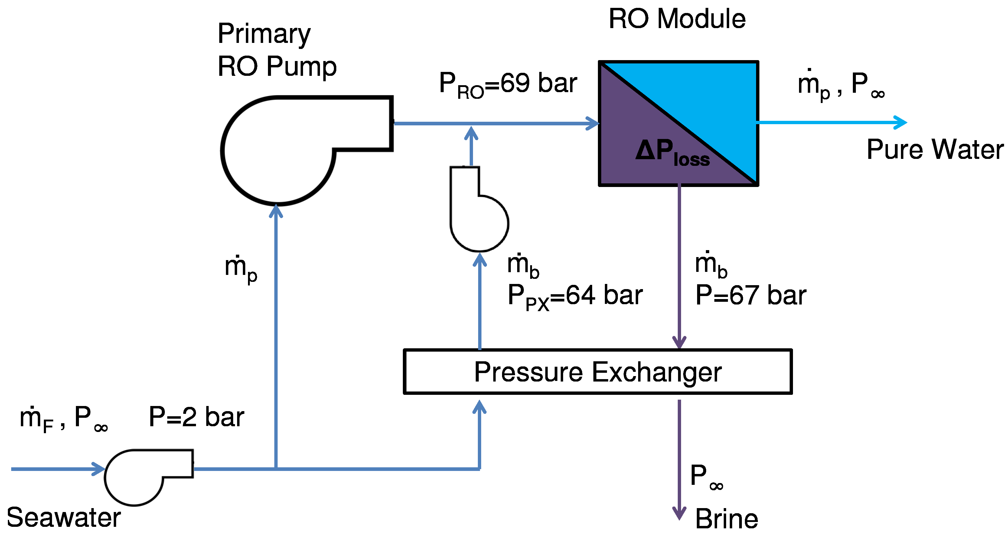
The pressure recovery step requires equal mass flow rates between the brine and feed stream, so the feed stream is split and only a portion goes through the pressure exchanger. The feed pump pressurizes the rest of the feed. Two minor pumps are needed as well, one for circulating the feed, bringing it to a pressure of 2 bar, and another to finish pressurizing the portion of water that passes through the pressure exchanger. The system diagram is shown in
Figure 22.
Figure 22.
Flow path diagram of reverse osmosis (RO) desalination.
Figure 22.
Flow path diagram of reverse osmosis (RO) desalination.
The entropy generation is calculated for each component as explained in the component sections (
Table 10), using entropy equations for pumping, chemical disequilibrium of brine, and for the pressure exchanger, compression and depressurizing. The entropy generation across the RO membrane can be calculated by summing the entropy generation caused by depressurizing the product stream as it passes from high to low pressure across the membrane with the compositional entropy change at the high pressure as evaluated from Equation (
12):
where the entropy,
s, is a function of temperature, salinity, and pressure, but pressure dependence is neglected for this nearly incompressible situation. The entropy generation from the pressure exchanger is calculating assuming compressing and depressurizing steps, and is explained in [
16].
As with MVC, the electricity for the RO unit first must be provided by converting the heat input at a given temperature to electrical work via the organic Rankine cycle. The results from the model are as follows (
Table 11).
Table 11.
Reverse osmosis modeling results.
Table 11.
Reverse osmosis modeling results.
| Output | Symbol | Value |
|---|
| Specific electricity consumption | | 2.35 kWh/m3 |
| RO unit Second Law efficiency | | 31.9% |
| Total Second Law efficiency, | | 17.3% |
| Total Second Law efficiency, | | 15.3% |
| Total Second Law efficiency, | | 10.8% |
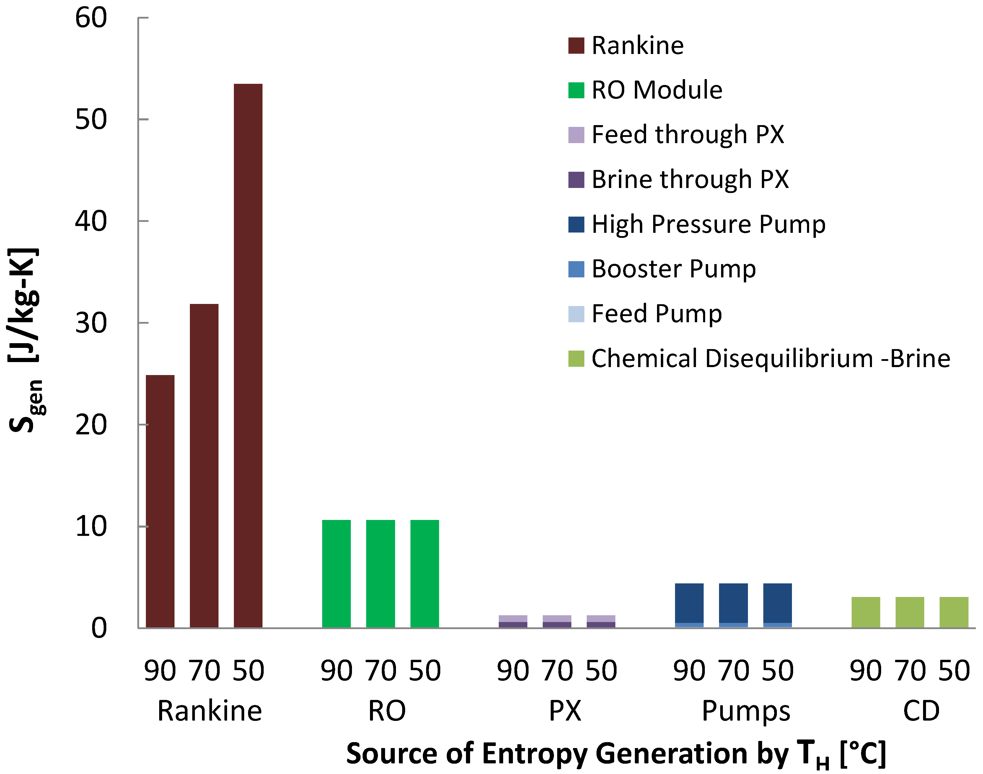
Figure 23.
Entropy generation per kilogram product water produced in each reverse osmosis component for all four temperatures modeled.
Figure 23.
Entropy generation per kilogram product water produced in each reverse osmosis component for all four temperatures modeled.
As seen in
Figure 23, the use of the Rankine cycle dominates the entropy generation for waste heat powered reverse osmosis. The next dominant source of entropy generation is across the RO module, and is significantly caused by the RO pressure (69 bar) being well above the osmotic pressure of seawater (27 bar), which is applied because the osmotic pressure grows as the salinity increases through the module, and because excess pressure is often used to increase the flow rate through the membrane, reducing needed membrane area. This can be improved by having multiple stages at different pressures [
44], reducing recovery (and thus brine salinity) and top pressure, batch processes where pressure is increased over time [
45], and other methods. The next dominant source of entropy generation is the high pressure pump, with the feed and booster pumps playing fairly insignificant roles. Chemical disequilibrium is the next major source of entropy generation, which is very high in RO due to the relatively good efficiency overall.
As seen in the case of MVC, the reduced performance of the Rankine cycle at lower temperatures causes the performance of RO to decrease.
6. Applicability of Analysis to Systems of Different Costs and Sizes
The effect of energy costs and system size on the efficiency of desalination plants must be understood to apply the results of this study to practical systems. The cost breakdown and data from existing plants can be examined to show the wide applicability of the thermodynamic analysis of this study.
Lower energy costs, which may occur in low temperature waste heat applications, reduce the need for energy efficient design. This affects the expenditure for heat exchanger area, which represents a trade off between large capital costs or large energy costs [
46]. Heat exchangers are used in all heat transfers between feed, brine, and product water and from the top heater providing waste heat. As the analysis in this paper shows, the entropy production is largely due to heat transfer across temperature gradients. However, because the heat exchanger and efficiency trade off is universal for all thermally-powered desalination technologies, all exhibit the same trend when energy costs are reduced. Furthermore, a cost analysis shows that the heat exchanger area in representative systems is a small part of total cost of water (<
) [
17], which means the optimal area changes only little with large changes in the unit price of energy [
17]. Comprehensive data on desalination plant sizes shows that for plants online now, MSF, MED, and RO systems of the same size but in regions of different typical energy cost vary very little in efficiency, almost always remaining withing
of their individual average ranges [
47,
48].
The efficiencies of online desalination plants varies only mildly across system sizes covering multiple orders of magnitude. For example, with few exemptions, the GOR of MSF plants varies within 7 and 10 for plants between 10,000 and 800,000
/day [
48], and modern RO unit energy use spans a range of
–
for plants ranging from 600
/day to 500,000
/day [
48]. Furthermore, the differences correlate strongly with size, with plants of similar sizes varying even less. Desalination systems do not get worse with increasing size, so the small MVC, MSVMD, and HDH systems modeled maintain or improve their efficiencies for large sizes. However, the comparison is limited for small systems, as MSF and MED systems of the types modeled change dramatically at small sizes, reducing the number of stages to 2–3 for the few installations below 1000
/day [
49]. The RO model is not always applicable below 50
/day as these plants may lack pressure recovery [
48], and some instances of HDH and multistage membrane distillation systems can be extremely small, with real systems below even 1
/day, while still providing GOR values similar to those in this paper [
50].
7. Technology Comparison
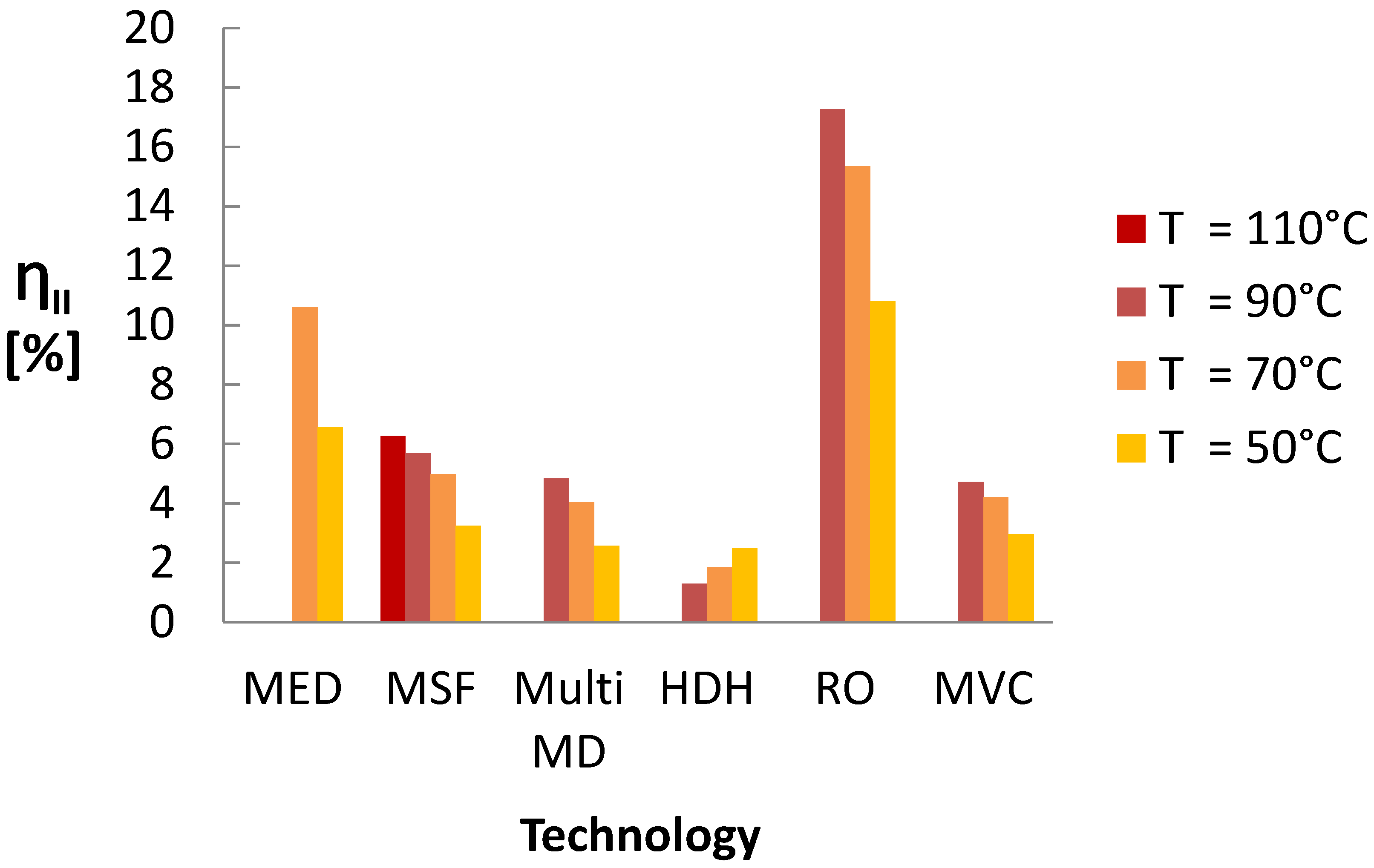
A summary of the Second Law efficiency from the previous modeling for each technology by heat source temperature is given in
Figure 24. The models used shared approximations and assumptions and shared real-world methods for modifying systems for lower temperatures.
The waste heat driven desalination technology with the highest Second Law efficiency, by a large margin, was RO, despite the entropy generated in the ORC. The next highest technology was MED, which could approach RO using recent advancements with adsorption cycles [
25]. MVC, MSF, and MSVMD had similar performances. The similarity in performance and efficiency trends for MSF and MSVMD was expected due to the thermodynamic similarity between the MSVMD and MSF technologies. Notably, while a stand-alone MVC system is known to have a higher efficiency than other thermal technologies [
16], when paired with an ORC, the efficiency of the MVC system decreases significantly, making MVC performance worse than that of MED but comparable to that of MSF and MSVMD. A simple closed cycle open water HDH system without moist air extractions, has lower efficiency than other thermal technologies at high waste heat temperatures. However, HDH efficiency at
= 50
was comparable to MSF, MSVMD and ORC-MVC [
33], and HDH systems with extractions can demonstrate much higher thermodynamic efficiency [
51].
Figure 24.
Second Law efficiency in each technology for all four temperatures modeled.
Figure 24.
Second Law efficiency in each technology for all four temperatures modeled.
In considering applications for these technologies operating on seawater, a dominant consideration is the system size, since some technologies are more scalable than others. MSF and MED plants are generally complex and require very large capital costs, especially due to the large heat exchanger areas [
49]. Overall, RO with a Rankine cycle is the most efficient for all system sizes: only other constraints such as relatively cheap energy or fouling issues could make the competitors a better choice [
52].
8. Comparison of Entropy Generation in Desalination System Components at Different Temperatures
Sources of Entropy Generation for All Desalination Technologies, Sorted by Largest Maximum Contribution.
- (1)
Temperature Gradients Across Heat Exchangers (In order from most to least : Feed Heaters, Stages or Effects, Top Heaters, Condensers, Regenerators,).
- (2)
Rankine Cycle Losses.
- (3)
Temperature Disequilibrium of Product and Brine
- (4)
Compressors (MVC)
- (5)
Phase Change (Flashing etc.)
- (6)
RO Module
- (7)
Throttling/Expansion
- (8)
Pumping Losses (RO)
- (9)
Chemical Disequilibrium of Brine
Entropy generation was much greater in the thermal technologies, and was generally due to unbalanced heat exchange and temperature gradients in heat exchangers.
The variation in sources of entropy generation between different temperature cases was almost entirely localized to certain system components. The entropy generation for the stages of MSF, MED, and MSVMD changed little between the four temperature scenarios, including in stage sub-components such as the MD module, the MED effects, and the MSF feed heaters and evaporator. For lower top temperatures, the number of stages was also reduced to keep the temperature differences between stages approximately constant. The distillate production rates for these stages changed little as well. For components with heat exchangers involving the distillate, such as the feed heaters, the distillate flow rates were so much smaller than the feed flow rate that, in all cases changed little.
However, for components where the entropy generation occurred in the feed or brine streams, tremendous increases in specific entropy generation occurred at lower temperature for the thermal technologies. The reduction in top temperature reduces recovery, causing relatively very large brine and feed flow rates: in these streams entropy is generated from the conditions (e.g., temperature change from conduction across a temperature gradient), but since
is normalized by
, significantly more entropy is generated per kilogram product water produced. For example, in MSF the entropy generation in the brine heater went from minor to being the largest contribution. In all thermal technologies, the reduced recovery causes an increase in entropy generation for temperature disequilibrium of the brine, again since a larger volume of brine is mixing with the ocean water. This relative flow rate effect also increased the entropy generation in the condenser for MED. The reduced recovery is a natural feature of lower source temperature systems, and is difficult to reduce as that would require increased performance and investment in the stage components, increasing the stage number and reducing temperature differences in the stage heat exchangers. As the stage performance changes little at lower temperature, while other components perform much worse, it hardly makes sense to focus investment in the stages, further limiting the ability to increase recovery with lower temperature heat sources. The lower temperatures also performed worse because at lower temperatures, more entropy is generated by heat transfer across a temperature gradient, as made apparent by the equation for
in
Table 1.
For electrically powered desalination technologies, entropy generation increased at lower temperatures due to the decreased efficiency of ORCs at lower driving temperature differences. The efficiency of the ORC significantly dominated their performance. Overall, the efficiency of RO and MVC did not vary quite as much with temperature as the efficiencies of the thermal desalination technologies, but the variation was proportionally very similar.
Entropy generation from chemical disequilibrium actually decreased for the lower temperature cases, since the recovery was reduced. Since this is a result of the concentration of brine, it was only proportionally significant for the most efficient systems, such as in RO.
Overall, most of the entropy generation in all these systems occurs due to heat transfer across temperature gradients in heat exchangers. This is seen in the feed heater, brine heater, and regenerator in MSF, the feed heaters and condenser in MED, and the humidifier and dehumidifier in HDH. Other methods experience lower losses for a few reasons. Where phase change occurs, temperature gradients can be small due to very high heat transfer coefficients. For mechanical systems such as pumps and compressors, technically it is easier to avoid losses with well-engineered components.
9. Conclusions
The impact of source temperature on six waste heat driven desalination technologies was studied. Through component level analysis, the impact on entropy generation within the components was identified which provides useful insight for how to adapt these technologies for lower temperature heat sources.
In comparing the technologies, reverse osmosis paired with an ORC had by far the highest Second Law efficiency.
Generally, at lower source temperatures, all technologies decreased in efficiency, especially the thermal ones. However, HDH experienced the opposite trend, improving performance when the top and bottom temperatures are close together: this occurs because the enthalpy of moist air is nonlinear with temperature, inducing larger temperature differences in the dehumidifier when the temperature range is broader, which leads to higher entropy generation. For that reason, HDH systems with injection and extraction (not considered here) are preferred in practice.
The efficiencies and this analysis were found to be applicable across a wide range of system sizes. HDH, MVC, RO, and multistage MD systems scaled to small sizes (<100 ) especially well.
Component-level entropy generation exhibited consistent trends. For the thermal technologies, entropy generation due to heat transfer across temperature gradients dominated; this occurred in the various heaters, regenerators, condensers, and other heat exchangers. As top temperatures decreased, overall entropy generation increased because the reduced recoveries increased feed and brine flow rates, causing significantly more entropy generation in those feed heat exchangers in particular. Meanwhile, in the product stream, including that in stages and effects of MSF, MED, and MSVMD. Increased temperature differences across heat exchangers also contributed substantially to the decreased performance at lower temperatures, as did heat transfer at lower temperatures.
For the electrically driven technologies, entropy generation in the ORCs dominated, and contributed to differences between different source temperatures. Entropy generation did not change for the components of the electrical technologies when the source temperature was varied.


