Information Dynamics in the Interaction between a Prey and a Predator Fish

Abstract

Accessing information efficiently is vital for animals to make the optimal decisions, and it is particularly important when they are facing predators. Yet until now, very few quantitative conclusions have been drawn about the information dynamics in the interaction between animals due to the lack of appropriate theoretic measures. Here, we employ transfer entropy (TE), a new information-theoretic and model-free measure, to explore the information dynamics in the interaction between a predator and a prey fish. We conduct experiments in which a predator and a prey fish are confined in separate parts of an arena, but can communicate with each other visually and tactilely. TE is calculated on the pair’s coarse-grained state of the trajectories. We find that the prey’s TE is generally significantly bigger than the predator’s during trials, which indicates that the dominant information is transmitted from predator to prey. We then demonstrate that the direction of information flow is irrelevant to the parameters used in the coarse-grained procedures. We further calculate the prey’s TE at different distances between it and the predator. The resulted figure shows that there is a high plateau in the mid-range of the distance and that drops quickly at both the near and the far ends. This result reflects that there is a sensitive space zone where the prey is highly vigilant of the predator’s position.

1. Introduction

Information dynamics play a crucial role for animals from both a behavioral and ecological perspective. When animals are foraging, mating or selecting a potential home site, information is the crucial currency to find the optimal option [1]. In particular, accessing information efficiently can be a matter of survival when the animals are confronted with predators.

In collective animal groups, such as bird flocks, fish schools and ant colonies, a necessary condition to maintain group cohesion is that information can be efficiently accessed by the individuals [2,3]. An impressive example is a flock of birds exhibiting striking airborne formations, which is believed to be a result of the local interaction between individuals [4,5,6]. In this example, the flow of information between interacting individuals determines the relationship between an individual’s spatial position and its effective leadership role [7]. When there is an environmental perturbation, such as a predator approaching, it is found that animals exhibit some group-level cognition to avoid the risks, such as a “wave of agitation” in a fish school [8]. Therefore, exploring the flow of information may infer the connection between the local information dynamics and the group intelligence.

Predation is a ubiquitous phenomenon in the natural world. In this situation, it is advantageous for prey to remain informed. For example, it is commonly seen that in a group of birds, some individuals keep their heads up to scan for approaching predators and play the roles of guards. It is widely observed in birds and mammals that individuals in a group devote progressively less time to be in a vigilant state as group size increases [9].

Information theory is a branch of applied mathematics involving the quantification of information [10,11,12]. It was developed by Claude E. Shannon [10,11] to study communications in electrical engineered systems and has now broadened to find applications in many other areas, including evolution [13], neurobiology [14,15], the function of molecular codes [13,16] and thermal physics [17]. Transfer entropy (TE), a recent development by Thomas Schreiber [18], is an information-theoretic and model-free tool to measure the information transmitted between a source and a destination in a dynamic process. The TE approach now has been used in measuring information flow in the physiology process of neuron dynamics in brain [14,15]. It has also been used in measuring information flow in the information transmitted in a flock in a dynamic process [7] and between a fish and a robot replica [19,20].

Wang et al. [7] applied TE and a related measure, active information storage, to study the spatiotemporal dynamics of swarms. They investigated two scenarios of the three-zone swarming model; one was concerned with the propagation of perturbations from the periphery in one group, and the other was concerned with the information dynamics when three separate groups merge. Their work validated the TE approach in the social interactions.

Recently, Butail et al. [19] studied the interaction between a zebrafish and a life-sized replica and between two live fish. The trajectory data were recorded when the fish swam in two separated regions in a tank. By applying TE to measure the interactions, they found that the dominant flow of information is from the replica to the fish. Their work laid the foundation of using TE as a measure of information flow in predation behaviors.

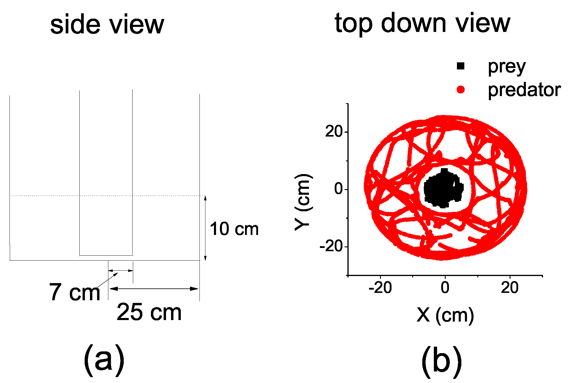
In this paper, we take a step further to utilize TE to explore the information dynamics in the interaction between a predator and a prey fish. We conduct experiments with a prey and a predator fish, which are confined separately in an arena, yet they can communicate with each other visually and tactilely. The information-theoretic tool is applied directly to the coarse-grained trajectories to reveal the hidden structure of the information dynamics in the predation interaction of fish.

The paper is organized as follows. In Section 2, we briefly introduce TE and its related concepts. Section 3 presents the materials and methods used to conduct the experiments. Before presenting the major results of TE, we present the details of the coarse-grained procedure in Section 4, which is a key step in applying this tool. Section 5 contains the major results of TE, including the comparison between the prey’s TE and the predator’s. To evaluate the sensitivity of the result, we calculate the difference between the TE of the two fish in a range of values of parameters used in the coarse-grained procedures. To further explore the space structure of the information dynamics, we calculate the prey’s TE at different distances between the two fish. Section 6 is the discussion and conclusion.

2. Preliminaries on Information Theory

The fundamental concept in information theory is the Shannon entropy [10,11], which measures the uncertainties associated with a random variable.

$$H\left(X\right)=-\sum _{x\in \chi }p\left(x\right){\text{log}}_{a}p\left(x\right),$$

(1)

where $p\left(x\right)$ is the probability mass function of a random variable X that can take a value in set χ, and the sum extends to all states x that X can assume. The constant base a depends on the unit chosen (for instance, $a=2$ for bits, and we omit it in the following text for convenience). The conditional entropy measures the remaining uncertainty of X if Y is given, with Y taking values in the set: $\mathcal{Y}$.

$$\begin{array}{c}\hfill H\left(X\right|Y)=-\sum _{x\in \chi }\sum _{y\in \mathcal{Y}}p(x,y)\text{log}p\left(x\right|y).\end{array}$$

(2)

The concept of mutual information measures the amount of information that one random variable contains about the other random variable. It is defined as:

$$\begin{array}{c}\hfill I(X;Y)=\sum _{x\in \chi }\sum _{y\in \mathcal{Y}}p(x,y)\text{log}\frac{p(x,y)}{p\left(x\right)p\left(y\right)}.\end{array}$$

(3)

If the value of mutual information is larger than zero, this means that the random variables are correlated.

The conditional mutual information between X and Y given Z (with Z taking values in $\mathcal{Z}$) is:

$$\begin{array}{c}\hfill I(X;Y|Z)=\sum _{x\in \chi }\sum _{y\in \mathcal{Y}}\sum _{z\in \mathcal{Z}}p(x,y,z)\text{log}\frac{p(x,y|z)}{p\left(x\right|z\left)p\right(y\left|z\right)}.\end{array}$$

(4)

It measures the reduction in the uncertainty of X due to knowledge of Y when Z is given. It also satisfies $I(X;Y|Z)\ge 0$, and the equality holds when X and Y are conditionally independent given Z.

Mutual information (including the conditional one) only measures the static statistical correlation of two distributions; therefore, it does not contain any dynamic information of the process. In order to incorporate the dynamic structure into these concepts, transition probabilities under the consideration of the Markov process is applied.

Consider a stationary Markov process of order k, so the probability of finding X in state $x_{n+1}$ is independent of the state $x_{n-k}$. This can be expressed as $p\left(x_{n+1}\right|x_n,x_{n-1},...,x_{n-k+1})=p\left(x_{n+1}\right|x_n,x_{n-1},...,x_{n-k})$, where n is a time index. For an initial study, we consider the $k=1$ case in this study.

TE was introduced by Schreiber [18], which is a model-free and theoretic measure of information transfer. It quantifies the information transmitted between a source node Y and a destination node X that is not contained in the past state of the destination X. The formula of transfer entropy is:

$$\begin{array}{c}\hfill TE(Y\to X)=\sum _{x_n\in \chi }\sum _{y_n\in \mathcal{Y}}\sum _{x_{n+1}\in \chi }p(x_{n+1},x_n,y_n)\text{log}\frac{p\left(x_{n+1}\right|x_n,y_n)}{p\left(x_{n+1}\right|x_n)}.\end{array}$$

(5)

The definition implies $TE(Y\to X)\ne TE(X\to Y)$.

Although TE is widely used, we should be cautious that in some cases, the nonzero of TE only reflects spurious correlation, which is resulted by imperfect observations of states [21]. We address this point by calculating it at different sets of coarse-grained parameters to eliminate the spurious correlation.

3. Materials and Methods

3.1. Animal

The prey (Rhodeus ocellatus, 1.53 ± 0.08 cm) and the predator (Channa argus, 9.31 ± 0.24 cm) had been maintained in a big holding tank separately for two weeks to acclimatize to the environments. Each predator fish had been starved for 48 hours before experiments. The holding tank, with a size of 150 L, was kept in a constant temperature room of 25 °C. The average swimming speed of the predator fish was 3.4 ± 1.7 cm/s, while the prey’s was 5.9 ± 2.0 cm/s. We found that the prey fish preferred to stay away from the predator, while the predator seemed to be moving aimlessly during the experiments. The fish were collected under the permission of the fisheries administrative institution of Chongqing City, which is responsible for the regulation of local fishes. All procedures were conducted in accordance with the national animal regulations, and the project was approved by the National Natural Science Foundation of China (No. 31172096) and Chongqing Normal University.

3.2. Experimental Setup

A circular arena, with a radius of 25 cm and a water depth of 10 cm, was divided into two concentric areas (see Figure 1a). The central circular area, with 7 cm in radius, was the prey fish’s space, and the concentric angular ring area, with a radius from 7 to 25 cm, was the predator’s space. Because fish can respond to stimuli from lateral lines and vision [22], we cut many small holes, with a diameter of about 0.3 cm each, in the transparent barrier ring. These holes were evenly distributed at a density of about $614/{\text{m}}^2$. Therefore, the barrier allowed the perturbation of water to ripple through it, so the fish in the separate areas could communicate with each other tactilely.

The setup was designed to be symmetrical in space and to take the different sizes of the predator and prey fish into account. The whole experimental setup was placed in a water tank to keep the environment in the whole area constant.

Figure 1. Arena and example trajectories. (a) Arena used in the experiments. The prey fish was in the smaller central circular area with a radius of 7 cm, while the predator fish was in the concentric angular ring area with a radius from 7 to 25 cm. The two fish were separated by a transparent barrier ring, with many small holes in it. The depth of water is 10 cm. (b) Example trajectories of the two fish. The trajectories were segments of Trial 4.

Figure 1. Arena and example trajectories. (a) Arena used in the experiments. The prey fish was in the smaller central circular area with a radius of 7 cm, while the predator fish was in the concentric angular ring area with a radius from 7 to 25 cm. The two fish were separated by a transparent barrier ring, with many small holes in it. The depth of water is 10 cm. (b) Example trajectories of the two fish. The trajectories were segments of Trial 4.

3.3. Experimental Procedure

The experiments were carried out at a constant temperature room of 25 °C. A prey was placed in the arena (smaller circular area) for 8 hours for acclimatization, and then, a predator was transferred from a holding tank with a hand net to the arena (concentric angular ring area). The relative long habituation time for the prey was selected according to the pilot studies. The prey fish took time to relax from an agitated state when they were first transferred to the arena. It was found that after 8 hours, the average swimming speed and the ratio of moving-to-stationary of the prey became stable. This procedure was performed in physiological and behavioral experiments of fish [23,24], with the habituation time ranging from 4 to 24 hours. We filmed the pair for 1 hour consecutively at 25 frames or 33 frames per second. To achieve statistical power, we conducted 5 trials of different pairs of prey and predator in the same condition. Because the predators often showed some explorative behaviors when they were first transferred to the arena, the initial 60 seconds of video clips were omitted. Video data were post-processed by a target-tracking system (EthoVision XT 9.0, Noldus Information Technology, Wageningen, The Netherlands) to output the trajectories of the two fishes.

On very few occasions, the tracking system failed to detect a fish position. We replaced the missing data with the average values of the data right before and after the moment.

4. Coarse-Grained in Space and Time

In order to employ TE, we had to convert the continuous coordinates to discrete ones and average the time series in a suitable time interval.

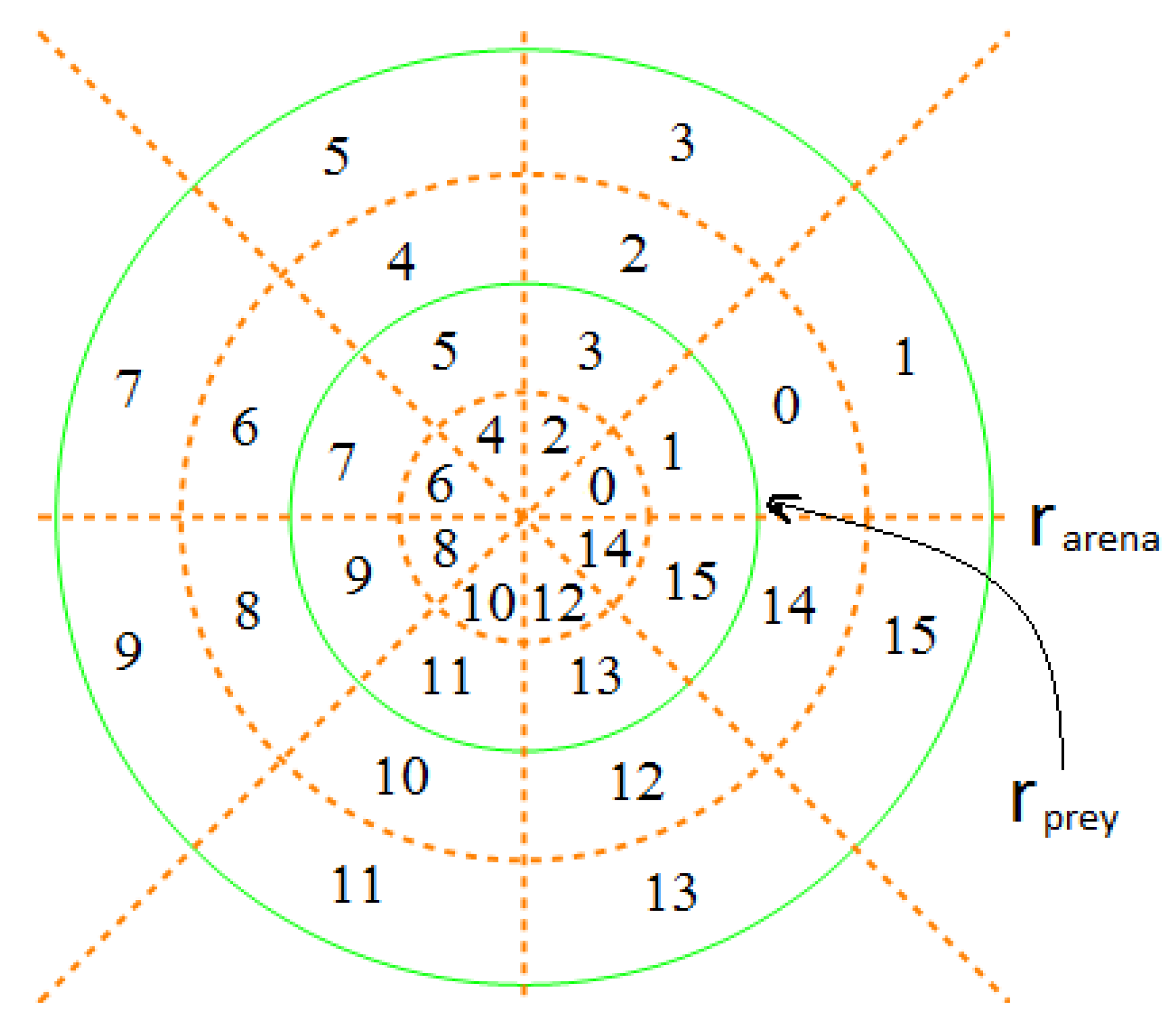
We first divided the entire circular space of the arena over the polar angle into n equal parts, so that the circular space of the prey was divided into n equal sectors and the annulus space of the predator was divided into n equal annular sectors. We continued to divide the sectors and the annular sectors by partitioning the radius. The radius of the sectors $r_{prey}$ and the annular sectors $r_{arena}-r_{prey}$ were equally partitioned into m parts, respectively. Consequently, the space was divided into cells (either a sector or an angular sector) with a common polar angle. However, the radii of the cells are different. The radius was $r_{prey}/m$ in the prey’s space, while it was $(r_{arena}-r_{prey})/m$ in the predator’s space. We denoted this mode of space division by $n\times m$ (see Figure 2). The different sizes of the cell took into account the different size of the fish.

Figure 2. Space-division mode $8\times 2$. The two solid green circles defined the space boundaries for the prey and predator fish, respectively. The dotted brown lines divided the whole space over the polar angle into eight sectors, and the dotted brown circles continued to partition the radius into two equal parts for the prey and the predator, respectively. Each cell, either being a sector or an annular sector, shared a common polar angle of $2\pi /8$. However, the radius of the cells in the prey’s space was $r_{prey}/2$ and in the predator’s space was $(r_{arena}-r_{prey})/2$. Consequently, both the prey and the predator could assume 16 possible states in this space division mode.

Figure 2. Space-division mode $8\times 2$. The two solid green circles defined the space boundaries for the prey and predator fish, respectively. The dotted brown lines divided the whole space over the polar angle into eight sectors, and the dotted brown circles continued to partition the radius into two equal parts for the prey and the predator, respectively. Each cell, either being a sector or an annular sector, shared a common polar angle of $2\pi /8$. However, the radius of the cells in the prey’s space was $r_{prey}/2$ and in the predator’s space was $(r_{arena}-r_{prey})/2$. Consequently, both the prey and the predator could assume 16 possible states in this space division mode.

The reaction time of fish is about 0.1 to 0.2 s, depending on the position and amplitude of the stimulus [25]. Therefore, we devised time intervals τ = 0.1 or 0.2 s to make the time discrete. Because the speed of fish is about a few body lengths per second [26], we devised a corresponding space division mode, so that the fish can reach a different cell in a time interval τ.

Given the coarse-grained space and time, we could translate the fish’s continuous trajectory into a discrete time and space series. Each fish’s raw trajectory data were first averaged in the time interval τ along the trial to obtain a discrete time series, then the (average) position in each time interval was placed in the corresponding labeled cell. In the coarse-grained space, the fish’s position was represented by a single number. This procedure is an essential step to apply TE, which relies on the mass probabilities of the relevant quantities; see Equation (5).

Example 1. Suppose that a series of trajectory data of prey fish, which is sampled with 33 frames per second, is {(2.25, 3.78), (4.57, −3.36), (−5.31, 2.86), (4.39, −1.28), (2.34, −6.21), (4.33, 2.15)}. Let us assume $\tau =0.1$ s, and the space division mode is $8\times 2$. We first average the trajectory data in the time interval τ (every three points are averaged to one), which becomes {(0.50, 1.09), (3.69, −1.78)}. Then, these average coordinate points are mapped to the corresponding labeled cells, and the final coarse-grained sequence is {(2), (9)}, which is discrete in time and space.

5. Results

In the experiments, the prey was agitated when the predator approached, while the predator seemed to move aimlessly most of the time. These observations were consistent with the quantitative measuring by TE.

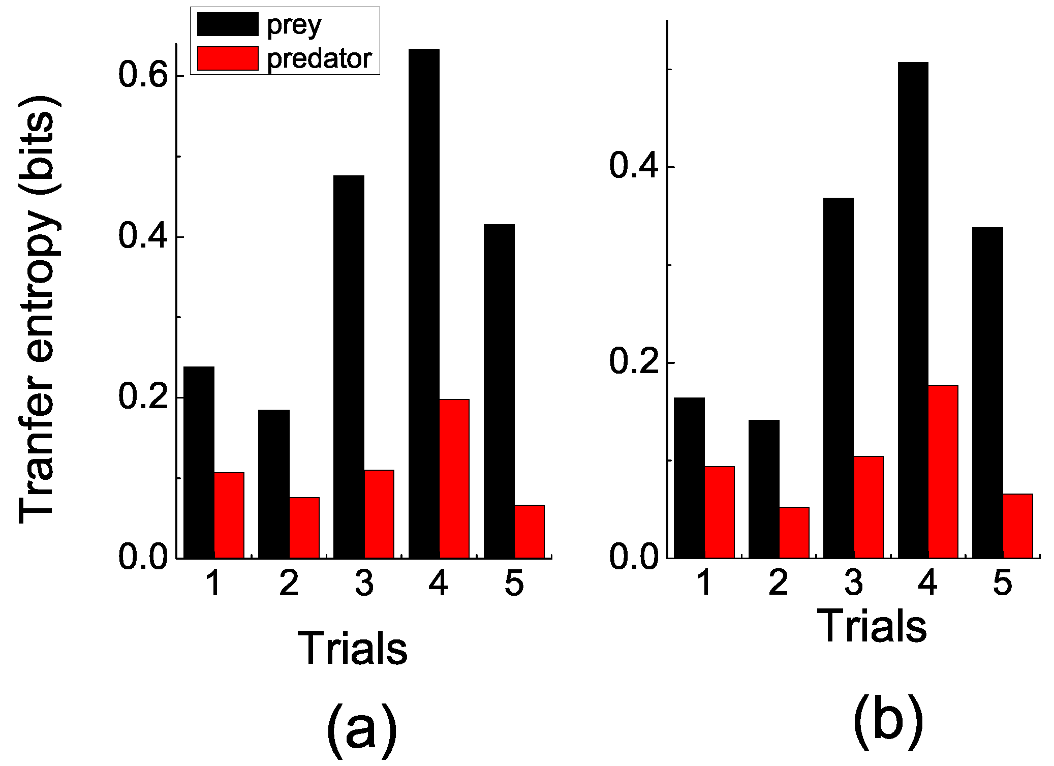
Figure 3 shows that the TE of the prey fish (information flows from the predator to the prey) was significantly larger than the TE of the predator fish (information flows from the prey to the predator). In order to eliminate spurious correlations, two sets of coarse-grain parameters (time intervals τ and space division modes $m\times n$) were selected. In Figure 3a, the space division mode is $40\times 10$, which resulted in 400 cells in each fish’s space, and the trajectories’ data were averaged in the interval of 0.1 s. In Figure 3b, the space division mode was $20\times 7$, and the data were averaged in the interval of 0.2 s.

Figure 3. (color online) Transfer entropy. (a) $\tau =0.1$ s, space division mode was $40\times 10$. (b) $\tau =0.2$ s, space division mode was $20\times 7$. This clearly shows that the prey’s transfer entropy (TE) (black bar) was significantly larger than the predator’s (red bar) over trials. Additionally, this pattern emerged when TE was computed on different sets of the coarse-grained parameters. This result indicates that more information was transmitted from predator to prey than vice versa.

Figure 3. (color online) Transfer entropy. (a) $\tau =0.1$ s, space division mode was $40\times 10$. (b) $\tau =0.2$ s, space division mode was $20\times 7$. This clearly shows that the prey’s transfer entropy (TE) (black bar) was significantly larger than the predator’s (red bar) over trials. Additionally, this pattern emerged when TE was computed on different sets of the coarse-grained parameters. This result indicates that more information was transmitted from predator to prey than vice versa.

However, no matter which set of coarse-grained parameters was chosen, a pattern emerged, which showed that the prey’s TE was generally significantly larger than the predator’s. Recalling the probabilistic property of TE, the results indicated that the position of the prey was more predicable given the position of the predator than vice versa. The low awareness of the predator to the prey may result from a low level of hunger, and this physiology state is related to complex environmental factors, such as water temperature [27].

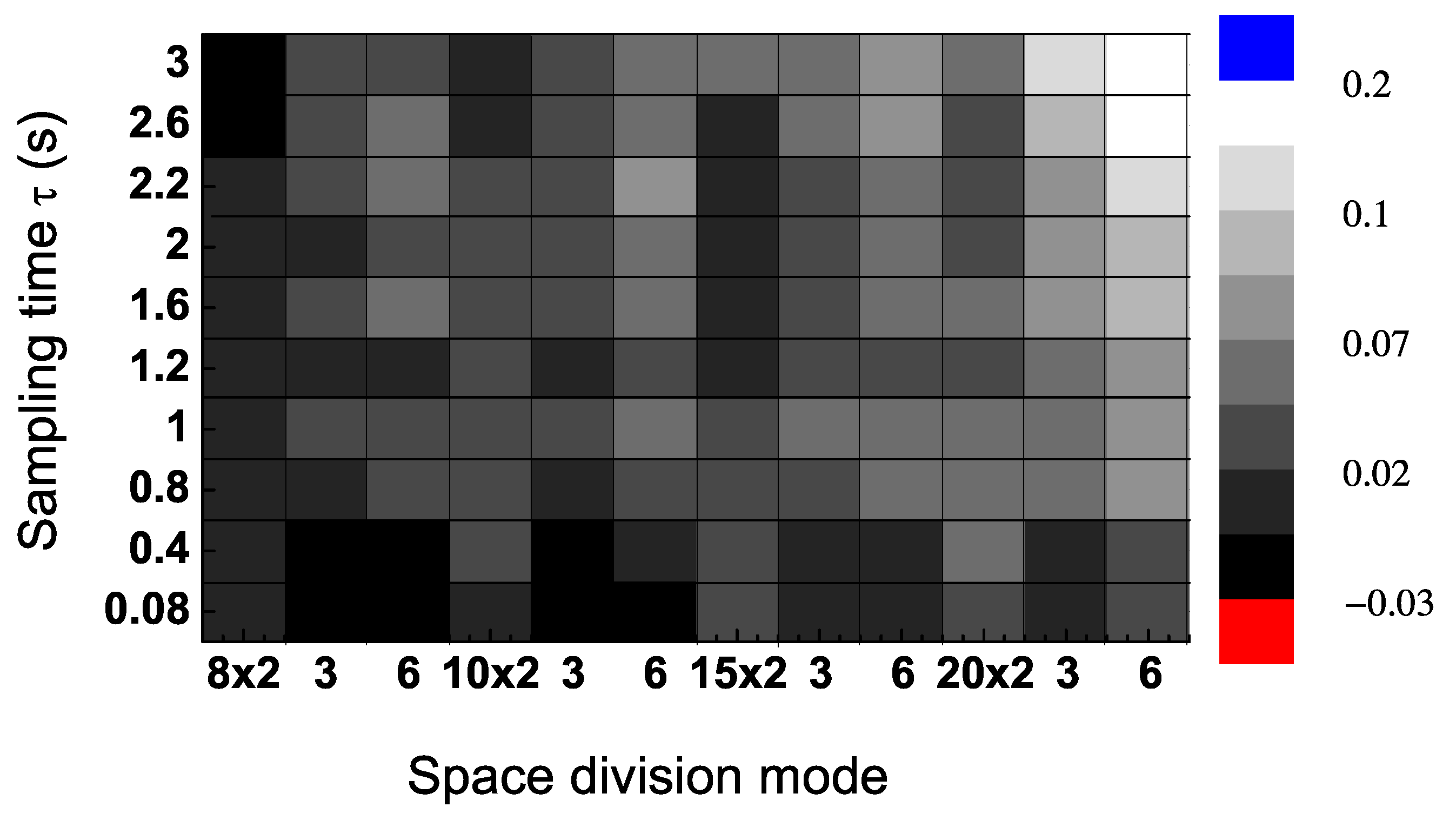
To evaluate the sensitivity of the dominant flow of information, we calculated ${\text{TE}}_{prey}-{\text{TE}}_{predator}$ in a range of values of sampling time intervals τ and space division modes $n\times m$. The results in Figure 4 were calculated from Trial 2 (randomly chose) in Figure 3. This shows that the direction of information flow, measured as the difference between the TE in each direction, is positive in most areas of the contour figure. In particular, the results are positive for values of the sampling time interval larger than 0.4 s (Figure 4).

Figure 4. Transfer entropy (TE) differences (${\text{TE}}_{prey}-{\text{TE}}_{predator}$) for a single trial (Trial 2 in Figure 3) for a range of values of sampling time τ and space division modes (which are 8 × 2, 8 × 3, 8 × 6, 10 × 2, etc.).

Figure 4. Transfer entropy (TE) differences (${\text{TE}}_{prey}-{\text{TE}}_{predator}$) for a single trial (Trial 2 in Figure 3) for a range of values of sampling time τ and space division modes (which are 8 × 2, 8 × 3, 8 × 6, 10 × 2, etc.).

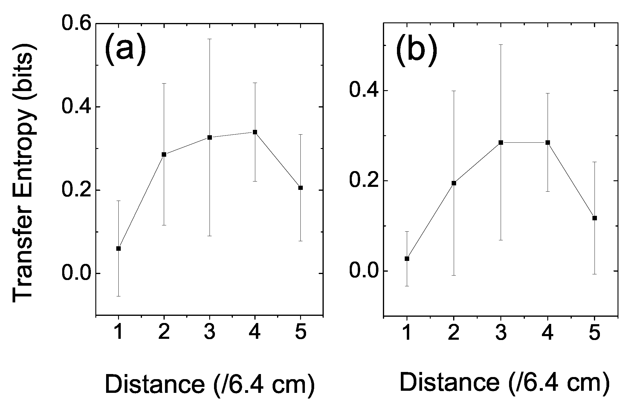
In order to explore the space structure of the information dynamics, we further investigated the relationship between the prey’s TE and the distance between the two fish [28]. The distance space was divided into five divisions; therefore, each division was comprised of a space distance of ((7 + 25)/5 =) 6.4 cm. In calculating the prey’s TE, we first clarified the events according to their distances. Then, we could count the frequencies of these events and calculate the relevant joint and conditioned probabilities according to Equation (5). Since TE is a statistical measure, we ignored the very rare events (less than 50) to reduce fluctuations when the distance between the fish reached zero or 32 cm. Two sets of coarse-grained parameters, the same as in Figure 3, were applied. Figure 5 shows the space structure of the information dynamics in the interaction between a prey and a predator fish. In Figure 5a, $\tau =0.1$ s, and space division mode was $40\times 10$; whereas, in Figure 5b, $\tau =0.2$ s, and space division mode was $20\times 7$. The results were averaged over trials. There is a high plateau at the mid-range distance in the figure and that drops quickly at both the near and far ends. It is not surprising that the prey’s TE dropped to a base value at the two ends; because on rare occasions, the prey allowed the predator to approach very near. If the predator stayed too far away, the prey paid little attention to the predator. This situation also resulted in a very low TE. No matter what set of parameters was chosen, this pattern emerged. It indicated that there was a vigilant space zone of the prey fish, in which it responded sensitively to the predator’s position.

Figure 5. The prey’s TE versus the distance between it and the predator. (a) $\tau =0.1$ s, space-division mode was $40\times 10$. (b) $\tau =0.2$ s, space division mode was $20\times 7$. The error bar was the standard deviation among trials. The high plateau in the mid-range distance reflects the vigilant space zone of the prey, in which it responded sensitively to the predator’s position.

Figure 5. The prey’s TE versus the distance between it and the predator. (a) $\tau =0.1$ s, space-division mode was $40\times 10$. (b) $\tau =0.2$ s, space division mode was $20\times 7$. The error bar was the standard deviation among trials. The high plateau in the mid-range distance reflects the vigilant space zone of the prey, in which it responded sensitively to the predator’s position.

6. Discussion and Conclusion

In this study, we conducted experiments on the predation behaviors between a prey and a predator fish to explore information dynamics in the process. Then, we applied a new information-theoretic measure, TE, to investigate information flow between them. In the experiments, a prey and a predator fish were confined in separate parts of an arena. The fish could not confront each other directly, but they could communicate visually and tactilely. TE was applied to the coarse-grained trajectory data of the two fish. We found that the prey’s TE was generally significantly larger than the predator’s over trials, and this pattern emerged no matter what set of coarse-grained parameters was chosen. This indicated that the prey was more vigilant about the predator’s position than vice versa. In order to explore the space structure of this information dynamics, we further measured the relationship of prey’s TE and the distance between the two fish. In Figure 5, we found a high plateau in the mid-range of the distance. This high plateau reflected the vigilant space zone of the prey in which it responded to the predator’s position actively.

Each one of the five trials in the study was comprised of a one-hour recording of the trajectories (25 or 33 frames per second) of the two fish. We assumed this amount of data is sufficient to give the conclusions with statistical significance. However, more works are needed to validate the general conclusions (e.g., applying different configurations of the experimental arena, exploring different state spaces of fish, investigating different species of fish). Another issue is a psychology effect in the experiments, which should be considered in the experiment design in the future. It can be imagined that the fish may realize the experimental setup forbidding their confrontation in the observation time and adjust their behaviors to this learning. One way to eliminate this effect is to shorten the duration of each trial and to conduct more trials at the same time to achieve statistical significance [19].

It was found that the interaction between a prey and a predator fish surpassed usual logical expectations [29]. The complex dynamic scenario required advanced tools to measure the hidden dynamic structures during the predation process. A very similar information theoretic tool was symbolic transfer entropy [30], which estimates TE by adopting a technique of symbolization. This approach relies on comparing the values of local neighbors [31]; that is the reason why it can work in the presence of noise. The local order patterns are then translated into symbolic sequences, so the probability of a symbol can be computed from the relative frequency of the symbol in the sequence. A key parameter in this approach is the embedding dimension, which determines the scope of local neighbors, which is very relevant to the space division mode defined in this paper. Theoretically, a fine-grained space-division mode, as the large embedding dimension, can preserve the detailed local information embedded in the raw data to the coarse-grained (symbolic) sequences. In practice, this procedure always brings out problems on computability and statistics. It is a trade-off between the theoretical requirements and the practical abilities in choosing appropriate parameters. However, in our work, the space division mode, paired with a time interval τ, was suggested based on a biological reasoning (see Section 4 for details). Given that the coordinate space was symmetrical in the arena and the only important variable was the distance between the prey and the predator, we assume that the symbolic transfer entropy approach cannot be directly applied in the coordinate space. Anyway, it would be interesting to apply it in the speed space in the future.

Compared with the prey’s high TE values, we assumed the predator had a low hunger level. Therefore, if we can change the physiological state of the predator, it might increase its attention to the prey, thus increasing the predator’s TE. However, there might exist another possibility. It was observed that larger prey groups, particularly bird flocks, were preferentially attacked [32]. Therefore, the asymmetrical TE distribution in Figure 3 can also be explained by the low interest of the predator to follow only one prey. It would be worth investigating the effects of a population of prey on predator behaviors.

Predatory behaviors are traditionally studied by unassisted observations [9,33]. In this paper, we provided a new method that brings out quantitative results. We hoped this method can be a complementary way to study vigilance behaviors.