Local Fractional Homotopy Perturbation Method for Solving Non-Homogeneous Heat Conduction Equations in Fractal Domains

Abstract

In this article, the local fractional Homotopy perturbation method is utilized to solve the non-homogeneous heat conduction equations. The operator is considered in the sense of the local fractional differential operator. Comparative results between non-homogeneous and homogeneous heat conduction equations are presented. The obtained result shows the non-differentiable behavior of heat conduction of the fractal temperature field in homogeneous media.

1. Introduction

Entropy in the thermodynamics is considered as the state function of a thermodynamic system. The entropy production in one-dimensional heat conduction in the hard-particle gas was considered in [1]. The maximum and minimum entropy productions in heat conduction problems were presented in [2,3]. The entropy generation in one-dimensional conduction was discussed in [4].

Recently, the entropy production via fractional order calculus [5,6,7,8,9,10] was suggested in [11]. The entropy production in fractional diffusion equation was proposed in [12,13]. The entropy analysis in fractional dynamical systems was presented in [14]. However, the above entropy process is differentiable. There may be non-differentiable entropy production in heat conduction of the fractal temperature field in homogeneous media [15]. Especially the non-homogeneous heat conduction equation (NHEC) in fractal domain was written as follows [16]:

$$\frac{{\partial }^{\epsilon }\text{Φ}\left(\mu ,\tau \right)}{\partial {\tau }^{\epsilon }}-\frac{{\partial }^{2\epsilon }\text{Φ}\left(\mu ,\tau \right)}{\partial {\mu }^{2\epsilon }}=F_{\epsilon }\left(\mu \right),\tau >0,\mu \in R,0<\epsilon <1,$$

(1)

subject to the initial condition

$$\text{Φ}\left(\mu ,0\right)=H_{\epsilon }\left(\mu \right),$$

(2)

where $F_{\epsilon }\left(\mu \right)$ is heat generation rate and the time and space operators are considered in the sense of local fractional differential operator (LFDO). The operator was applied to describe the non-differentiable equations, such as Laplace [16], diffusion [17], oscillator [18], heat [16,19], Boussinesq [20], wave [16,21], Burgers [22] and parabolic Fokker–Planck [23] defined on Cantor sets. The comparison between diffusion problem via local fractional time- and space- derivative operators and classical one was presented in [24]. The fractal heat conduction equation with the help of local fractional time- and space- derivative operators was discussed by using the local fractional Laplace operator [25]. For more applications in integral transforms and fluid mechanics, see [26,27,28].

More recently, the homotopy perturbation method via local fractional homotopy perturbation (LFDO) method, proposed by authors in [29], was applied to solve the wave equations involving the Cantor sets. The homotopy perturbation method, structured by He in [30], was applied to heat transfer [31], water wave theory [32] and diffusion problems [33]. In this manuscript, we will implement the technology to solving the NHCEs in fractal domain. The structure of this article is as follows. In Section 2, we introduce the basic theory of LFDO with applications to special functions defined on Cantor sets. In Section 3, the local fractional homotopy perturbation method is analyzed. The non-differentiable solutions (NSs) for the NHCEs are given in Section 4. In Section 5 the comparison between NHCE and homogeneous heat conduction equation (HHCE) is discussed. Finally, Section 6 is devoted to the conclusions.

2. The LFDO

In this section, we present the basic theory of LFDO [16,17,18,19,20,21,22,23,24,25,26,27,28,29].

The LFDO of $\text{Θ}\left(\mu \right)$ of ε order ($0<\epsilon \le 1)$ is defined by

$$\frac{{\partial }^{\epsilon }\text{Θ}\left(\mu \right)}{\partial {\mu }^{\epsilon }}\left|{}_{\mu ={\mu }_0}\right.=\underset{\mu \to {\mu }_0}{lim}\frac{{\text{Δ}}^{\epsilon }\left(\text{Θ}\left(\mu \right)-\text{Θ}\left({\mu }_0\right)\right)}{{\left(\mu -{\mu }_0\right)}^{\epsilon }},$$

(3)

where ${\text{Δ}}^{\epsilon }\left(\text{Θ}\left(\mu \right)-\text{Θ}\left({\mu }_0\right)\right)\cong \Gamma \left(1+\epsilon \right)\Delta \left(\Theta \left(\mu \right)-\Theta \left({\mu }_0\right)\right)$.

The properties of the LFDO are as follows [16]:

(a)

$D^{\left(\epsilon \right)}\left[\Phi \left(\mu \right)\pm \Theta \left(\mu \right)\right]=D^{\left(\epsilon \right)}\Phi \left(\mu \right)\pm D^{\left(\epsilon \right)}\Theta \left(\mu \right)$,

(b)

$D^{\left(\epsilon \right)}\left[\Phi \left(\mu \right)\Theta \left(\mu \right)\right]=\left[D^{\left(\epsilon \right)}\Phi \left(\mu \right)\right]\Theta \left(\mu \right)+\Phi \left(\mu \right)\left[D^{\left(\epsilon \right)}\Theta \left(\mu \right)\right]$,

(c)

$D^{\left(\epsilon \right)}\left[\Phi \left(\mu \right)/\Theta \left(\mu \right)\right]=\left\{\left[D^{\left(\epsilon \right)}\Phi \left(\mu \right)\right]\Theta \left(\mu \right)-\Phi \left(\mu \right)\left[D^{\left(\epsilon \right)}\Theta \left(\mu \right)\right]\right\}/{\Theta }^2\left(\mu \right)$, provided $\Theta \left(\mu \right)\ne 0$.

The basic operations of the local fractional differential operators (LFDOs) of the non-differentiable functions (NDFSs) defined on fractal sets are listed in Table 1.

Table 1. The basic operations of local fractional differential operator (LFDO) of non-differentiable functions (NDFs) defined on fractal sets.

$\Phi \left(\mu \right)$	$D^{\left(\epsilon \right)}\Phi \left(\mu \right)$	Special functions defined on Cantor sets
C	0
${\mu }^{k\epsilon }/\Gamma \left(1+k\epsilon \right)$	${\mu }^{\left(k-1\right)\epsilon }/\Gamma \left(1+\left(k-1\right)\epsilon \right)$
$E_{\epsilon }\left({\mu }^{\epsilon }\right)$	$E_{\epsilon }\left({\mu }^{\epsilon }\right)$	$E_{\epsilon }\left({\mu }^{\epsilon }\right)={\displaystyle \sum _{k=0}^{\infty }}\frac{{\mu }^{k\epsilon }}{\Gamma \left(1+k\epsilon \right)}$
$E_{\epsilon }\left(-{\mu }^{\epsilon }\right)$	$-E_{\epsilon }\left(-{\mu }^{\epsilon }\right)$
${sin}_{\epsilon }\left({\mu }^{\epsilon }\right)$	${cos}_{\epsilon }\left({\mu }^{\epsilon }\right)$	${sin}_{\epsilon }\left({\mu }^{\epsilon }\right)={\displaystyle \sum _{k=0}^{\infty }}{\frac{{\left(-1\right)}^k{\mu }^{\left(2k+1\right)\epsilon }}{\Gamma \left(1+\left(2k+1\right)\epsilon \right)}}_{,}$ ${cos}_{\epsilon }\left({\mu }^{\epsilon }\right)={\displaystyle \sum _{k=0}^{\infty }}\frac{{\left(-1\right)}^k{\mu }^{2k\epsilon }}{\Gamma \left(1+2k\epsilon \right)}$
${cos}_{\epsilon }\left({\mu }^{\epsilon }\right)$	$-{sin}_{\epsilon }\left({\mu }^{\epsilon }\right)$

Table 1. The basic operations of local fractional differential operator (LFDO) of non-differentiable functions (NDFs) defined on fractal sets.

$\Phi \left(\mu \right)$	$D^{\left(\epsilon \right)}\Phi \left(\mu \right)$	Special functions defined on Cantor sets
C	0
${\mu }^{k\epsilon }/\Gamma \left(1+k\epsilon \right)$	${\mu }^{\left(k-1\right)\epsilon }/\Gamma \left(1+\left(k-1\right)\epsilon \right)$
$E_{\epsilon }\left({\mu }^{\epsilon }\right)$	$E_{\epsilon }\left({\mu }^{\epsilon }\right)$	$E_{\epsilon }\left({\mu }^{\epsilon }\right)={\displaystyle \sum _{k=0}^{\infty }}\frac{{\mu }^{k\epsilon }}{\Gamma \left(1+k\epsilon \right)}$
$E_{\epsilon }\left(-{\mu }^{\epsilon }\right)$	$-E_{\epsilon }\left(-{\mu }^{\epsilon }\right)$
${sin}_{\epsilon }\left({\mu }^{\epsilon }\right)$	${cos}_{\epsilon }\left({\mu }^{\epsilon }\right)$	${sin}_{\epsilon }\left({\mu }^{\epsilon }\right)={\displaystyle \sum _{k=0}^{\infty }}{\frac{{\left(-1\right)}^k{\mu }^{\left(2k+1\right)\epsilon }}{\Gamma \left(1+\left(2k+1\right)\epsilon \right)}}_{,}$ ${cos}_{\epsilon }\left({\mu }^{\epsilon }\right)={\displaystyle \sum _{k=0}^{\infty }}\frac{{\left(-1\right)}^k{\mu }^{2k\epsilon }}{\Gamma \left(1+2k\epsilon \right)}$
${cos}_{\epsilon }\left({\mu }^{\epsilon }\right)$	$-{sin}_{\epsilon }\left({\mu }^{\epsilon }\right)$

3. Analysis of the Method

In this section the local fractional homotopy perturbation method [29] will be presented as follows.

The NHCE is written in the form

$$L_{\epsilon }\left({\Phi }^{\epsilon }\right)=0,$$

(4)

where $L_{\alpha }$ is a LFDO.

A convex non-differentiable homotopy ${\widehat{H}}_{\epsilon }\left(\Phi ,\theta ,\epsilon \right)$ is structured as follows:

$${\widehat{H}}_{\epsilon }\left(\Phi ,\theta ,\epsilon \right)={\Lambda }_{\epsilon }\left(L_{\epsilon }\left({\Phi }^{\epsilon }\right)-L_{\epsilon }\left({\Phi }_0^{\epsilon }\right)\right)+{\theta }^{\epsilon }{L}_{\epsilon }\left({\Phi }^{\epsilon }\right),\theta \in \left[0,1\right],$$

(5)

where ${\Lambda }_{\epsilon }={\left(1-\theta \right)}^{\epsilon }$ and ${\Phi }_0={\Phi }_0^{\epsilon }$ is an initial approximation of Equation (5).

Setting ${\widehat{H}}_{\epsilon }\left(\Phi ,\theta ,\epsilon \right)=0$, we obviously have

$${\widehat{H}}_{\epsilon }\left(\Phi ,0,\epsilon \right)=L_{\epsilon }\left({\Phi }^{\epsilon }\right)-L_{\epsilon }\left({\Phi }_0^{\epsilon }\right),$$

(6)

$${\widehat{H}}_{\epsilon }\left(\Phi ,1,\epsilon \right)=L_{\epsilon }\left({\Phi }^{\epsilon }\right).$$

(7)

In the structure of non-differentiable homotopy, the non-differentiable deformation is $L_{\epsilon }\left(\Phi \right)-L_{\epsilon }\left({\Phi }_0\right)$ and the non-differentiable homotopics is $L_{\epsilon }\left(\Phi \right)$.

With the help of the non-differentiable series [17], ${\Phi }^{\epsilon }$ can be expressed by

$${\Phi }^{\epsilon }=\sum _{j=0}^n{{\theta }^{j\epsilon }{\Phi }_j^{\epsilon }}_{.}$$

(8)

Making use of Equations (5) and (8), we obtain

$${\widehat{H}}_{\epsilon }\left(\Phi ,\theta ,\epsilon \right)={\Lambda }_{\epsilon }\left(L_{\epsilon }\left(\sum _{j=0}^n{\theta }^{j\epsilon }{\Phi }_j^{\epsilon }\right)-L_{\epsilon }\left({\Phi }_0^{\epsilon }\right)\right)+{\theta }^{\epsilon }{L}_{\epsilon }\left(\sum _{j=0}^n{\theta }^{j\epsilon }{\Phi }_j^{\epsilon }\right),$$

(9)

where ${\Lambda }_{\epsilon }={\left(1-\theta \right)}^{\epsilon }$.

Expanding $L_{\epsilon }\left({\Phi }^{\epsilon }\right)$ into a local fractional Taylor series, we have

$$\begin{array}{ccc}\hfill L_{\epsilon }\left({\Phi }^{\epsilon }\right)& =& L_{\epsilon }\left({\Phi }_0^{\epsilon }\right)+\frac{d^{\epsilon }\left(L_{\epsilon }\left({\Phi }_0^{\epsilon }\right)\right)}{d{\Phi }^{\epsilon }}\frac{{\left({\displaystyle \sum _{j=0}^n}{\theta }^j{\Phi }_j-{\Phi }_0\right)}^{\epsilon }}{\Gamma \left(1+\epsilon \right)}+O\left({\left(\sum _{j=0}^n{\theta }^j{\Phi }_j-{\Phi }_0\right)}^{\epsilon }\right)\hfill \\ \mathrm{(10)}& & =& L_{\epsilon }\left({\Phi }_0^{\epsilon }\right)+\frac{d^{\epsilon }\left(L_{\epsilon }\left({\Phi }_0^{\epsilon }\right)\right)}{d{\Phi }^{\epsilon }}\frac{\left({\displaystyle \sum _{j=0}^n}{\theta }^{j\epsilon }{\Phi }_j^{\epsilon }-{\Phi }_0^{\epsilon }\right)}{\Gamma \left(1+\epsilon \right)}+O\left({\left(\sum _{j=0}^n{\theta }^j{\Phi }_j-{\Phi }_0\right)}^{\epsilon }\right).\hfill \end{array}$$

such that

$$\begin{array}{c}{\widehat{H}}_{\epsilon }\left(\Phi ,\theta ,\epsilon \right)\hfill \\ ={\left(1-\theta \right)}^{\epsilon }\left(L_{\epsilon }\left({\Phi }^{\epsilon }\right)-L_{\epsilon }\left({\Phi }_0^{\epsilon }\right)\right)+{\theta }^{\epsilon }{L}_{\epsilon }\left({\Phi }^{\epsilon }\right)\hfill \\ \mathrm{(11)}& ={\left(1-\theta \right)}^{\epsilon }\left(L_{\epsilon }\left({\Phi }_0^{\epsilon }\right)+\frac{d^{\epsilon }\left(L_{\epsilon }\left({\Phi }_0^{\epsilon }\right)\right)}{d{\Phi }^{\epsilon }}\frac{\left({\displaystyle \sum _{j=0}^n}{\theta }^{j\epsilon }{\Phi }_j^{\epsilon }-{\Phi }_0^{\epsilon }\right)}{\Gamma \left(1+\epsilon \right)}+O\left({\left({\displaystyle \sum _{j=0}^n}{\theta }^j{\Phi }_j-{\Phi }_0\right)}^{\epsilon }\right)-L_{\epsilon }\left({\Phi }_0^{\epsilon }\right)\right)\hfill +{\theta }^{\epsilon }\left(L_{\epsilon }\left({\Phi }_0^{\epsilon }\right)+\frac{d^{\epsilon }\left(L_{\epsilon }\left({\Phi }_0^{\epsilon }\right)\right)}{d{\Phi }^{\epsilon }}\frac{\left({\displaystyle \sum _{j=0}^n}{\theta }^{j\epsilon }{\Phi }_j^{\epsilon }-{\Phi }_0^{\epsilon }\right)}{\Gamma \left(1+\epsilon \right)}+O\left({\left({\displaystyle \sum _{j=0}^n}{\theta }^j{\Phi }_j-{\Phi }_0\right)}^{\epsilon }\right)\right),\hfill \end{array}$$

which reduces to

$$\begin{array}{ccc}\hfill {\widehat{H}}_{\epsilon }\left(\Phi ,0,\epsilon \right)& =& L_{\epsilon }\left({\Phi }^{\epsilon }\right)-L_{\epsilon }\left({\Phi }_0^{\epsilon }\right)\hfill \\ & =& L_{\epsilon }\left({\Phi }_0^{\epsilon }\right)+\frac{d^{\epsilon }\left(L_{\epsilon }\left({\Phi }_0^{\epsilon }\right)\right)}{d{\Phi }^{\epsilon }}\frac{\left({\displaystyle \sum _{j=0}^n}{\theta }^{j\epsilon }{\Phi }_j^{\epsilon }-{\Phi }_0^{\epsilon }\right)}{\Gamma \left(1+\epsilon \right)}+O\left({\left(\sum _{j=0}^n{\theta }^j{\Phi }_j-{\Phi }_0\right)}^{\epsilon }\right)-L_{\epsilon }\left({\Phi }_0^{\epsilon }\right)\hfill \\ \mathrm{(12)}& & =& 0\hfill \end{array}$$

and

$$\begin{array}{ccc}\hfill {\widehat{H}}_{\epsilon }\left(\Phi ,1,\epsilon \right)& =& {\Lambda }_{\epsilon }\left(L_{\epsilon }\left({\Phi }^{\epsilon }\right)-L_{\epsilon }\left({\Phi }_0^{\epsilon }\right)\right)+{\theta }^{\epsilon }{L}_{\epsilon }\left({\Phi }^{\epsilon }\right)\hfill \\ & =& {\theta }^{\epsilon }{L}_{\epsilon }\left({\Phi }^{\epsilon }\right)\hfill \\ \mathrm{(13)}& & =& {\theta }^{\epsilon }\left(L_{\epsilon }\left({\Phi }_0^{\epsilon }\right)+\frac{d^{\epsilon }\left(L_{\epsilon }\left({\Phi }_0^{\epsilon }\right)\right)}{d{\Phi }^{\epsilon }}\frac{\left({\displaystyle \sum _{j=0}^n}{\theta }^{j\epsilon }{\Phi }_j^{\epsilon }-{\Phi }_0^{\epsilon }\right)}{\Gamma \left(1+\epsilon \right)}+O\left({\left(\sum _{j=0}^n{\theta }^j{\Phi }_j-{\Phi }_0\right)}^{\epsilon }\right)\right).\hfill \end{array}$$

Adopting Equations (12) and (13), we obtain

$${\theta }^{0\epsilon }:L_{\epsilon }\left({\Phi }^{\epsilon }\right)-L_{\epsilon }\left({\Phi }_0^{\epsilon }\right)=0,$$

(14)

$${\theta }^{1\epsilon }:L_{\epsilon }\left({\Phi }_0^{\epsilon }\right)+\frac{d^{\epsilon }\left(L_{\epsilon }\left({\Phi }_0^{\epsilon }\right)\right)}{d{\Phi }^{\epsilon }}\frac{{\Phi }_1^{\epsilon }}{\Gamma \left(1+\epsilon \right)}=0.$$

(15)

Here, Equation (15) is the Newton’s method of the LFDO and it is convergent.

Taking $\theta \to 1$, the approximate solution takes the form

$${\Phi }^{\epsilon }=\underset{\theta \to 1}{lim}\sum _{j=0}^{\infty }{\theta }^{j\epsilon }{\Phi }_j^{\epsilon }=\sum _{j=0}^{\infty }{\Phi }_j^{\epsilon }.$$

(16)

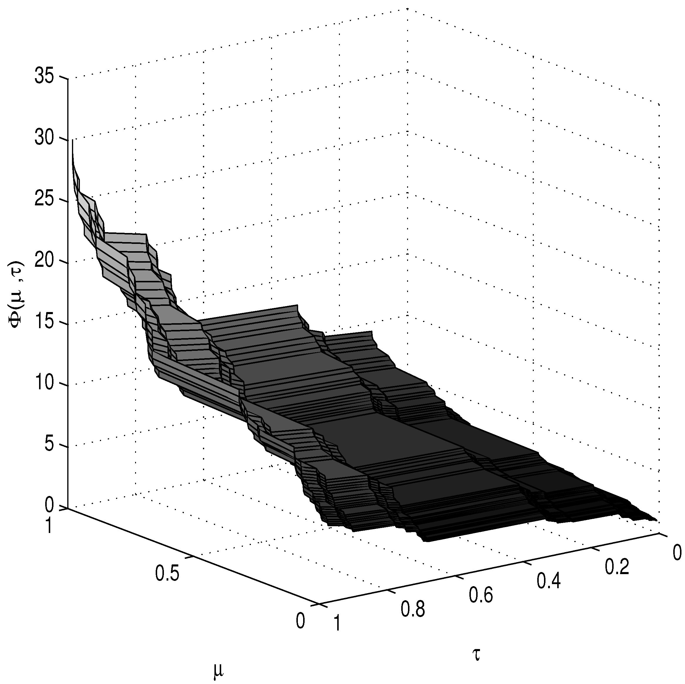
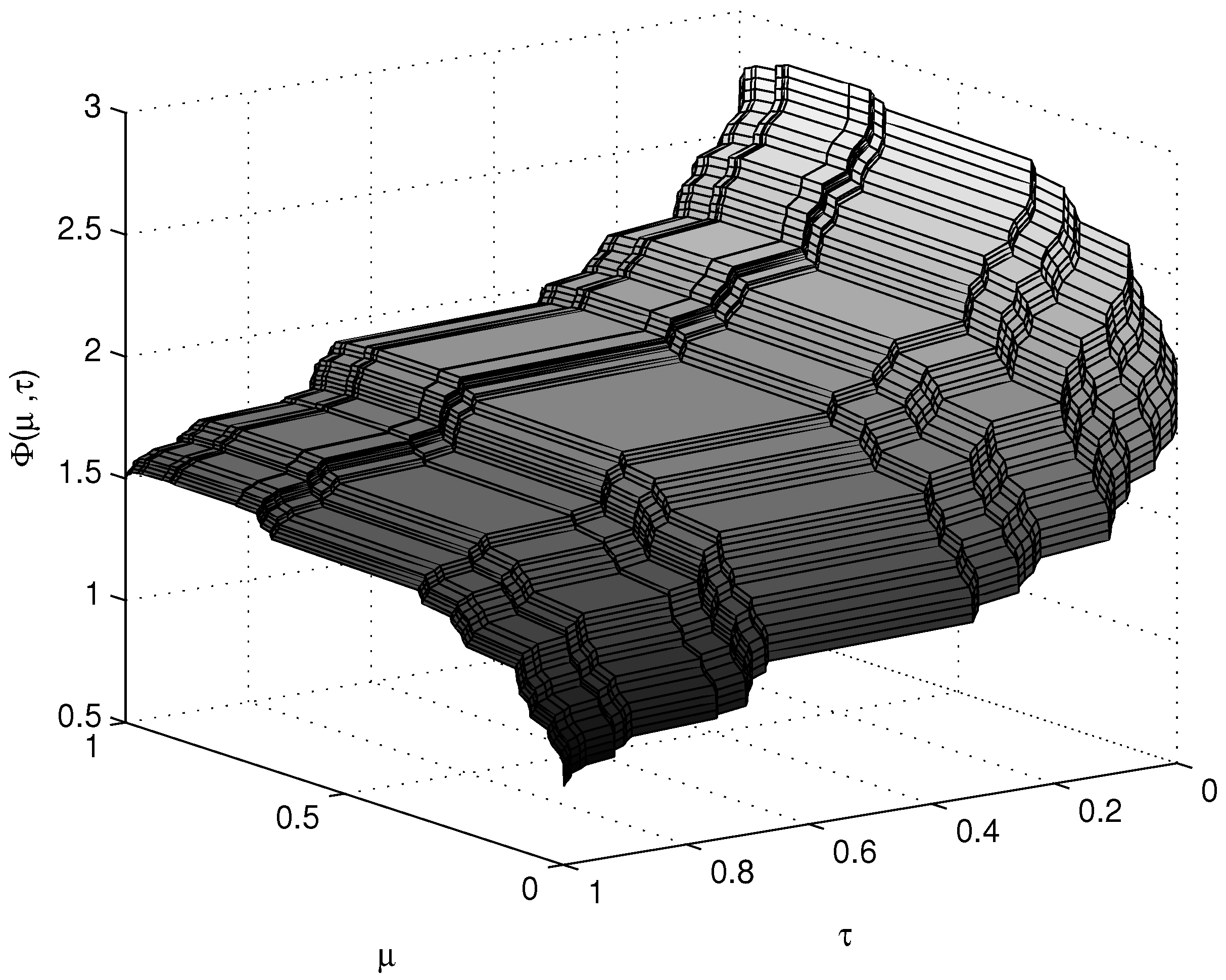
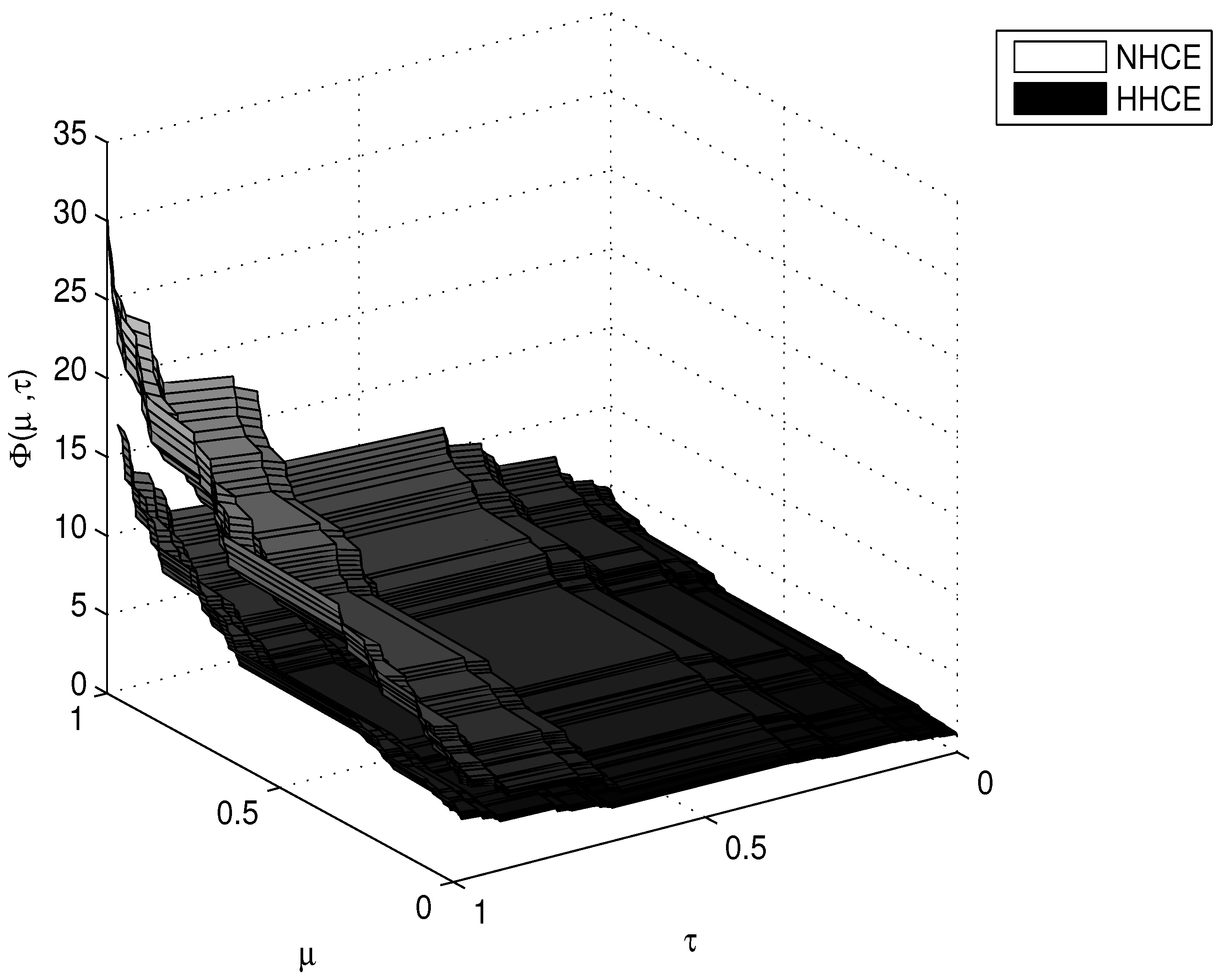
4. On Solutions of the NHCEs

In this section, the NSs of the NHCEs are discussed.

Let us consider the following NHCE with heat generation of non-differentiable type

$$\frac{{\partial }^{\epsilon }\Phi \left(\mu ,\tau \right)}{\partial {\tau }^{\epsilon }}-\frac{{\partial }^{2\epsilon }\Phi \left(\mu ,\tau \right)}{\partial {\mu }^{2\epsilon }}=E_{\epsilon }\left({\mu }^{\epsilon }\right),\tau >0,\mu \in R,$$

(17)

subject to the initial condition

$$\Phi \left(\mu ,0\right)=E_{\epsilon }\left({\mu }^{\epsilon }\right).$$

(18)

We can structure the non-differentiable homotopy in the form:

$$\frac{{\partial }^{\epsilon }\Phi \left(\mu ,\tau \right)}{\partial {\tau }^{\epsilon }}-\frac{{\partial }^{\epsilon }{\Phi }_0\left(\mu ,\tau \right)}{\partial {\tau }^{\epsilon }}={\theta }^{\epsilon }\left(\frac{{\partial }^{2\epsilon }\Phi \left(\mu ,\tau \right)}{\partial {\mu }^{2\epsilon }}+E_{\epsilon }\left({\mu }^{\epsilon }\right)-\frac{{\partial }^{\epsilon }{\Phi }_0\left(\mu ,\tau \right)}{\partial {\tau }^{\epsilon }}\right),$$

(19)

and the solution series with non-differentiable terms is presented as follows:

$$\Phi =\sum _{j=0}^{\infty }{\theta }^{j\epsilon }{\Phi }_j.$$

(20)

Submitting Equations (18) and (20) into Equation (19), we have

$$\begin{array}{c}\frac{{\partial }^{\epsilon }}{\partial {\tau }^{\epsilon }}\left[{\displaystyle \sum _{j=0}^{\infty }}{\theta }^{j\epsilon }{\Phi }_j\left(\mu ,\tau \right)\right]-\frac{{\partial }^{\epsilon }{\Phi }_0\left(\mu ,\tau \right)}{\partial {\tau }^{\epsilon }}={\theta }^{\epsilon }\left(\frac{{\partial }^{2\epsilon }}{\partial {\mu }^{2\epsilon }}\left[{\displaystyle \sum _{j=0}^{\infty }}{\theta }^{j\epsilon }{\Phi }_j\left(\mu ,\tau \right)\right]+E_{\epsilon }\left({\mu }^{\epsilon }\right)-\frac{{\partial }^{\epsilon }{\Phi }_0\left(\mu ,\tau \right)}{\partial {\tau }^{\epsilon }}\right)\hfill \end{array}$$

(21)

such that

$${\theta }^{0\epsilon }:\frac{{\partial }^{\epsilon }{\Phi }_0\left(\mu ,\tau \right)}{\partial {\tau }^{\epsilon }}-\frac{{\partial }^{\epsilon }{\Phi }_0\left(\mu ,\tau \right)}{\partial {\tau }^{\epsilon }}=0,{\Phi }_0\left(\mu ,0\right)=E_{\epsilon }\left({\mu }^{\epsilon }\right),$$

(22)

$${\theta }^{1\epsilon }:\frac{{\partial }^{\epsilon }{\Phi }_1\left(\mu ,\tau \right)}{\partial {\tau }^{\epsilon }}=\frac{{\partial }^{2\epsilon }{\Phi }_0\left(\mu ,\tau \right)}{\partial {\mu }^{2\epsilon }}+E_{\epsilon }\left({\mu }^{\epsilon }\right)-\frac{{\partial }^{\epsilon }{\Phi }_0\left(\mu ,\tau \right)}{\partial {\tau }^{\epsilon }},{\Phi }_1\left(\mu ,0\right)=0,$$

(23)

$${\theta }^{2\epsilon }:\frac{{\partial }^{\epsilon }{\Phi }_2\left(\mu ,\tau \right)}{\partial {\tau }^{\epsilon }}=\frac{{\partial }^{2\epsilon }{\Phi }_1\left(\mu ,\tau \right)}{\partial {\mu }^{2\epsilon }},{\Phi }_2\left(\mu ,0\right)=0,$$

(24)

$${\theta }^{3\epsilon }:\frac{{\partial }^{\epsilon }{\Phi }_3\left(\mu ,\tau \right)}{\partial {\tau }^{\epsilon }}=\frac{{\partial }^{2\epsilon }{\Phi }_2\left(\mu ,\tau \right)}{\partial {\mu }^{2\epsilon }},{\Phi }_3\left(\mu ,0\right)=0,$$

(25)

$${\theta }^{4\epsilon }:\frac{{\partial }^{\epsilon }{\Phi }_4\left(\mu ,\tau \right)}{\partial {\tau }^{\epsilon }}=\frac{{\partial }^{2\epsilon }{\Phi }_3\left(\mu ,\tau \right)}{\partial {\mu }^{2\epsilon }},{\Phi }_4\left(\mu ,0\right)=0$$

(26)

and so on.

Solving above systems, we present

$${\Phi }_0\left(\mu ,\tau \right)=E_{\epsilon }\left({\mu }^{\epsilon }\right),$$

(27)

$${\Phi }_1\left(\mu ,\tau \right)=\frac{2{\tau }^{\epsilon }}{\Gamma \left(1+\epsilon \right)}{E}_{\epsilon }\left({\mu }^{\epsilon }\right),$$

(28)

$${\Phi }_2\left(\mu ,\tau \right)=\frac{2{\tau }^{2\epsilon }}{\Gamma \left(1+2\epsilon \right)}{E}_{\epsilon }\left({\mu }^{\epsilon }\right),$$

(29)

$${\Phi }_3\left(\mu ,\tau \right)=\frac{2{\tau }^{3\epsilon }}{\Gamma \left(1+3\epsilon \right)}{E}_{\epsilon }\left({\mu }^{\epsilon }\right),$$

(30)

$${\Phi }_4\left(\mu ,\tau \right)=\frac{2{\tau }^{4\epsilon }}{\Gamma \left(1+4\epsilon \right)}{E}_{\epsilon }\left({\mu }^{\epsilon }\right)$$

(31)

and so on.

When $\theta \to 1$, from Equation (20) we obtain

$$\begin{array}{ccc}\hfill \Phi \left(\mu ,\tau \right)& =& \sum _{j=0}^{\infty }{\Phi }_j\left(\mu ,\tau \right)\hfill \\ \mathrm{(32)}& & =& 2E_{\epsilon }\left({\mu }^{\epsilon }\right)\left(\frac{{\tau }^{\epsilon }}{\Gamma \left(1+\epsilon \right)}+\frac{{\tau }^{2\epsilon }}{\Gamma \left(1+2\epsilon \right)}+\frac{{\tau }^{3\epsilon }}{\Gamma \left(1+3\epsilon \right)}+\frac{{\tau }^{4\epsilon }}{\Gamma \left(1+4\epsilon \right)}+...\right)+E_{\epsilon }\left({\mu }^{\epsilon }\right).\hfill \end{array}$$

Using Equation (32), we obtain the NS in closed form

$$\Phi \left(\mu ,\tau \right)=E_{\epsilon }\left({\mu }^{\epsilon }\right)\left(2\sum _{j=0}^{\infty }\frac{{\tau }^{j\epsilon }}{\Gamma \left(1+j\epsilon \right)}-1\right)=E_{\epsilon }\left({\mu }^{\epsilon }\right)\left(2E_{\epsilon }\left({\tau }^{\epsilon }\right)-1\right)$$

(33)

and the corresponding plot with fractal dimension $\epsilon =ln2/ln3$ is shown in Figure 1.

Figure 1. The solution for non-homogeneous heat conduction equation (NHCE) with heat generation of non-differentiable type when $\epsilon =ln2/ln3$.

Figure 1. The solution for non-homogeneous heat conduction equation (NHCE) with heat generation of non-differentiable type when $\epsilon =ln2/ln3$.

We consider the following NHCE with heat sink of non-differentiable type

$$\frac{{\partial }^{\epsilon }\Phi \left(\mu ,\tau \right)}{\partial {\tau }^{\epsilon }}-\frac{{\partial }^{2\epsilon }\Phi \left(\mu ,\tau \right)}{\partial {\mu }^{2\epsilon }}=-{cos}_{\epsilon }\left({\mu }^{\epsilon }\right),\tau >0,\mu \in R,$$

(34)

subject to the initial condition

$$\Phi \left(\mu ,0\right)={sin}_{\epsilon }\left({\mu }^{\epsilon }\right).$$

(35)

The non-differentiable homotopy is defined as follows:

$$\frac{{\partial }^{\epsilon }\Phi \left(\mu ,\tau \right)}{\partial {\tau }^{\epsilon }}-\frac{{\partial }^{\epsilon }{\Phi }_0\left(\mu ,\tau \right)}{\partial {\tau }^{\epsilon }}={\theta }^{\epsilon }\left(\frac{{\partial }^{2\epsilon }\Phi \left(\mu ,\tau \right)}{\partial {\mu }^{2\epsilon }}-{cos}_{\epsilon }\left({\mu }^{\epsilon }\right)-\frac{{\partial }^{\epsilon }{\Phi }_0\left(\mu ,\tau \right)}{\partial {\tau }^{\epsilon }}\right).$$

(36)

The solution series with non-differentiable terms takes the form:

$$\Phi =\sum _{j=0}^{\infty }{\theta }^{j\epsilon }{\Phi }_j.$$

(37)

Submitting Equations (18) and (20) into Equation (19), we obtain

$$\begin{array}{c}\frac{{\partial }^{\epsilon }}{\partial {\tau }^{\epsilon }}\left[{\displaystyle \sum _{j=0}^{\infty }}{\theta }^{j\epsilon }{\Phi }_j\left(\mu ,\tau \right)\right]-\frac{{\partial }^{\epsilon }{\Phi }_0\left(\mu ,\tau \right)}{\partial {\tau }^{\epsilon }}={\theta }^{\epsilon }\left(\frac{{\partial }^{2\epsilon }}{\partial {\mu }^{2\epsilon }}\left[{\displaystyle \sum _{j=0}^{\infty }}{\theta }^{j\epsilon }{\Phi }_j\left(\mu ,\tau \right)\right]-{cos}_{\epsilon }\left({\mu }^{\epsilon }\right)-\frac{{\partial }^{\epsilon }{\Phi }_0\left(\mu ,\tau \right)}{\partial {\tau }^{\epsilon }}\right).\hfill \end{array}$$

(38)

Due to Equation (38), we can structure a set of local fractional partial differential equations

$${\theta }^{0\epsilon }:\frac{{\partial }^{\epsilon }{\Phi }_0\left(\mu ,\tau \right)}{\partial {\tau }^{\epsilon }}-\frac{{\partial }^{\epsilon }{\Phi }_0\left(\mu ,\tau \right)}{\partial {\tau }^{\epsilon }}=0,{\Phi }_0\left(\mu ,0\right)={sin}_{\epsilon }\left({\mu }^{\epsilon }\right),$$

(39)

$${\theta }^{1\epsilon }:\frac{{\partial }^{\epsilon }{\Phi }_1\left(\mu ,\tau \right)}{\partial {\tau }^{\epsilon }}=\frac{{\partial }^{2\epsilon }{\Phi }_0\left(\mu ,\tau \right)}{\partial {\mu }^{2\epsilon }}-{cos}_{\epsilon }\left({\mu }^{\epsilon }\right)-\frac{{\partial }^{\epsilon }{\Phi }_0\left(\mu ,\tau \right)}{\partial {\tau }^{\epsilon }},{\Phi }_1\left(\mu ,0\right)=0,$$

(40)

$${\theta }^{2\epsilon }:\frac{{\partial }^{\epsilon }{\Phi }_2\left(\mu ,\tau \right)}{\partial {\tau }^{\epsilon }}=\frac{{\partial }^{2\epsilon }{\Phi }_1\left(\mu ,\tau \right)}{\partial {\mu }^{2\epsilon }},{\Phi }_2\left(\mu ,0\right)=0,$$

(41)

$${\theta }^{3\epsilon }:\frac{{\partial }^{\epsilon }{\Phi }_3\left(\mu ,\tau \right)}{\partial {\tau }^{\epsilon }}=\frac{{\partial }^{2\epsilon }{\Phi }_2\left(\mu ,\tau \right)}{\partial {\mu }^{2\epsilon }},{\Phi }_3\left(\mu ,0\right)=0,$$

(42)

$${\theta }^{4\epsilon }:\frac{{\partial }^{\epsilon }{\Phi }_4\left(\mu ,\tau \right)}{\partial {\tau }^{\epsilon }}=\frac{{\partial }^{2\epsilon }{\Phi }_3\left(\mu ,\tau \right)}{\partial {\mu }^{2\epsilon }},{\Phi }_4\left(\mu ,0\right)=0$$

(43)

and so on.

Solving above systems, we obtain

$${\Phi }_0\left(\mu ,\tau \right)={sin}_{\epsilon }\left({\mu }^{\epsilon }\right),$$

(44)

$${\Phi }_1\left(\mu ,\tau \right)=-\frac{{\tau }^{\epsilon }}{\Gamma \left(1+\epsilon \right)}\left[{sin}_{\epsilon }\left({\mu }^{\epsilon }\right)+{cos}_{\epsilon }\left({\mu }^{\epsilon }\right)\right],$$

(45)

$${\Phi }_2\left(\mu ,\tau \right)=\frac{{\tau }^{2\epsilon }}{\Gamma \left(1+2\epsilon \right)}\left[{sin}_{\epsilon }\left({\mu }^{\epsilon }\right)+{cos}_{\epsilon }\left({\mu }^{\epsilon }\right)\right],$$

(46)

$${\Phi }_3\left(\mu ,\tau \right)=-\frac{{\tau }^{3\epsilon }}{\Gamma \left(1+3\epsilon \right)}\left[{sin}_{\epsilon }\left({\mu }^{\epsilon }\right)+{cos}_{\epsilon }\left({\mu }^{\epsilon }\right)\right],$$

(47)

$${\Phi }_4\left(\mu ,\tau \right)=\frac{{\tau }^{4\epsilon }}{\Gamma \left(1+4\epsilon \right)}\left[{sin}_{\epsilon }\left({\mu }^{\epsilon }\right)+{cos}_{\epsilon }\left({\mu }^{\epsilon }\right)\right]$$

(48)

and so on.

When $\theta \to 1$, with the help of Equation (37), we have

$$\begin{array}{ccc}\hfill \Phi \left(\mu ,\tau \right)& =& \sum _{j=0}^{\infty }{\Phi }_j\left(\mu ,\tau \right)\hfill \\ \mathrm{(49)}& & =& {sin}_{\epsilon }\left({\mu }^{\epsilon }\right)+\left(\sum _{j=1}^{\infty }\frac{{(-1)}^j{\tau }^{j\epsilon }}{\Gamma \left(1+j\epsilon \right)}\right)\left[{sin}_{\epsilon }\left({\mu }^{\epsilon }\right)+{cos}_{\epsilon }\left({\mu }^{\epsilon }\right)\right].\hfill \end{array}$$

In view of Equation (49), we have the NS in closed form

$$\begin{array}{ccc}\hfill \Phi \left(\mu ,\tau \right)& =& \sum _{j=0}^{\infty }\frac{{(-1)}^j{\tau }^{j\epsilon }}{\Gamma \left(1+j\epsilon \right)}\left[{sin}_{\epsilon }\left({\mu }^{\epsilon }\right)+{cos}_{\epsilon }\left({\mu }^{\epsilon }\right)\right]-{cos}_{\epsilon }\left({\mu }^{\epsilon }\right)\hfill \\ \mathrm{(50)}& & =& E_{\epsilon }\left(-{\tau }^{\epsilon }\right)\left[{sin}_{\epsilon }\left({\mu }^{\epsilon }\right)+{cos}_{\epsilon }\left({\mu }^{\epsilon }\right)\right]-{cos}_{\epsilon }\left({\mu }^{\epsilon }\right).\hfill \end{array}$$

and the corresponding graph with fractal dimension $\epsilon =ln2/ln3$ is illustrated in Figure 2.

Figure 2. The solution for non-homogeneous heat conduction equation (NHCE) with heat sink of non-differentiable type when $\epsilon =ln2/ln3$.

Figure 2. The solution for non-homogeneous heat conduction equation (NHCE) with heat sink of non-differentiable type when $\epsilon =ln2/ln3$.

5. Discussion

In order to present the novel technology, we will discuss comparison between the NHCE and HHCE.

The HHCE (local fractional diffusion equation [29]) in fractal domain

$$\frac{{\partial }^{\epsilon }\Phi \left(\mu ,\tau \right)}{\partial {\tau }^{\epsilon }}-\frac{{\partial }^{2\epsilon }\Phi \left(\mu ,\tau \right)}{\partial {\mu }^{2\epsilon }}=0$$

(51)

is considered. The initial value condition (IVC) of Equation (51) is presented as follows [29]:

$$\Phi \left(\mu ,0\right)=E_{\epsilon }\left({\mu }^{\epsilon }\right).$$

(52)

The corresponding NS for the HHCE is presented as follows [29]:

$$\Phi \left(\mu ,\tau \right)=E_{\epsilon }\left({\mu }^{\epsilon }\right)E_{\epsilon }\left({\tau }^{\epsilon }\right).$$

(53)

Owing to the above, the comparative results for the NHCE and HHCE with the NSs are listed in Table 2.

Table 2. The comparative results for the HHCE and NHCE.

	PDEs	NSs
HHCE	$\frac{{\partial }^{\epsilon }\Phi \left(\mu ,\tau \right)}{\partial {\tau }^{\epsilon }}-\frac{{\partial }^{2\epsilon }\Phi \left(\mu ,\tau \right)}{\partial {\mu }^{2\epsilon }}=0$	$\Phi \left(\mu ,\tau \right)=E_{\epsilon }\left({\mu }^{\epsilon }\right)E_{\epsilon }\left({\tau }^{\epsilon }\right)$
NHCE	$\frac{{\partial }^{\epsilon }\Phi \left(\mu ,\tau \right)}{\partial {\tau }^{\epsilon }}-\frac{{\partial }^{2\epsilon }\Phi \left(\mu ,\tau \right)}{\partial {\mu }^{2\epsilon }}=E_{\epsilon }\left({\mu }^{\epsilon }\right)$	$\Phi \left(\mu ,\tau \right)=E_{\epsilon }\left({\mu }^{\epsilon }\right)\left(2E_{\epsilon }\left({\tau }^{\epsilon }\right)-1\right)$
IVCs	$\Phi \left(\mu ,0\right)=E_{\epsilon }\left({\mu }^{\epsilon }\right)$	$\Phi \left(\mu ,0\right)=E_{\epsilon }\left({\mu }^{\epsilon }\right)$

Table 2. The comparative results for the HHCE and NHCE.

	PDEs	NSs
HHCE	$\frac{{\partial }^{\epsilon }\Phi \left(\mu ,\tau \right)}{\partial {\tau }^{\epsilon }}-\frac{{\partial }^{2\epsilon }\Phi \left(\mu ,\tau \right)}{\partial {\mu }^{2\epsilon }}=0$	$\Phi \left(\mu ,\tau \right)=E_{\epsilon }\left({\mu }^{\epsilon }\right)E_{\epsilon }\left({\tau }^{\epsilon }\right)$
NHCE	$\frac{{\partial }^{\epsilon }\Phi \left(\mu ,\tau \right)}{\partial {\tau }^{\epsilon }}-\frac{{\partial }^{2\epsilon }\Phi \left(\mu ,\tau \right)}{\partial {\mu }^{2\epsilon }}=E_{\epsilon }\left({\mu }^{\epsilon }\right)$	$\Phi \left(\mu ,\tau \right)=E_{\epsilon }\left({\mu }^{\epsilon }\right)\left(2E_{\epsilon }\left({\tau }^{\epsilon }\right)-1\right)$
IVCs	$\Phi \left(\mu ,0\right)=E_{\epsilon }\left({\mu }^{\epsilon }\right)$	$\Phi \left(\mu ,0\right)=E_{\epsilon }\left({\mu }^{\epsilon }\right)$

The comparative results for the NHCE and HHCE with initial value condition (IVCs) are depicted in Figure 3.

Figure 3. The non-differentiable solutions (NSs) for the homogeneous heat conduction equation (HHCE) and non-homogeneous heat conduction equation (NHCE).

Figure 3. The non-differentiable solutions (NSs) for the homogeneous heat conduction equation (HHCE) and non-homogeneous heat conduction equation (NHCE).

When changing the fractal dimension from $ln2/ln3$ to 1, we have the conversational NHCE in the form

$$\frac{\partial \Phi \left(\mu ,\tau \right)}{\partial \tau }-\frac{{\partial }^2\Phi \left(\mu ,\tau \right)}{\partial {\mu }^2}=exp\left(\mu \right)$$

(54)

with the initial condition

$$\Phi \left(\mu ,0\right)=exp{\left(\mu \right)}_{,}$$

(55)

and the corresponding solution is written as follows:

$$\Phi \left(\mu ,\tau \right)=exp\left(\mu \right)\left(2exp\left(\tau \right)-1\right).$$

(56)

The comparison between the HHCEs with LFDO and conversational differential operator (CDO) is represented in Figure 4.

Figure 4. The comparison between the homogeneous heat conduction equations (HHCEs) within the different operators.

Figure 4. The comparison between the homogeneous heat conduction equations (HHCEs) within the different operators.

6. Conclusions

In our work we have utilized the local fractional homotopy perturbation method to implement the NHECs with the help of the local fractional time- and space-derivatives. The NSs for NHECs were presented and their charts of the special functions defined on Cantor sets with fractal dimension $\epsilon =ln2/ln3$ were displayed. The comparative results for the NHCE and HHCE were also discussed. The results illustrate the efficiency of the technology to solve the local fractional differentiable equations.

References

1. Grassberger, P.; Nadler, W.; Yang, L. Heat conduction and entropy production in a one-dimensional hard-particle gas. Phys. Rev. Lett. 2002, 89, 180601. [Google Scholar] [CrossRef]
2. Kim, S.K.; Lee, W.I. Solution of inverse heat conduction problems using maximum entropy method. Int. J. Heat Mass Transf. 2002, 45, 381–391. [Google Scholar] [CrossRef]
3. Kolenda, Z.; Donizak, J.; Hubert, J. On the minimum entropy production in steady state heat conduction processes. Energy 2004, 29, 2441–2460. [Google Scholar] [CrossRef]
4. Bautista, O.; Méndez, F.; Martinez-Meyer, J.L. (Bejan’s) early vs. late regimes method applied to entropy generation in one-dimensional conduction. Int. J. Therm. Sci. 2005, 44, 570–576. [Google Scholar] [CrossRef]
5. Tarasov, V.E. Fractional Dynamics: Applications of Fractional Calculus to Dynamics of Particles, Fields and Media; Springer: Berlin/Heidelberg, Germany, 2011. [Google Scholar]
6. Hristov, J. An approximate analytical (integral-balance) solution to a nonlinear heat diffusion equation. Therm. Sci. 2015, 19, 723–733. [Google Scholar] [CrossRef]
7. Ortigueira, M.D. Fractional Calculus for Scientists and Engineers; Springer: Berlin/Heidelberg, Germany, 2011. [Google Scholar]
8. Baleanu, D.; Machado, J.A.T.; Luo, A.C. Fractional Dynamics and Control; Springer: Berlin/Heidelberg, Germany, 2011. [Google Scholar]
9. Ubriaco, M.R. Entropies based on fractional calculus. Phys. Lett. A 2009, 373, 2516–2519. [Google Scholar] [CrossRef]
10. Kilbas, A.A.A.; Srivastava, H.M.; Trujillo, J.J. Theory and Applications of Fractional Differential Equations; Elsevier: Amsterdam, The Netherlands, 2006. [Google Scholar]
11. Essex, C.; Schulzky, C.; Franz, A.; Hoffmann, K.H. Tsallis and Rényi entropies in fractional diffusion and entropy production. Phys. A Stat. Mech. Appl. 2000, 284, 299–308. [Google Scholar] [CrossRef]
12. Li, X.; Essex, C.; Davison, M.; Hoffmann, K.H.; Schulzky, C. Fractional diffusion, irreversibility and entropy. J. Non-Equilib. Thermodyn. 2003, 28, 279–291. [Google Scholar] [CrossRef]
13. Magin, R.; Ingo, C. Entropy and information in a fractional order model of anomalous diffusion. Syst. Identif. 2012, 16, 428–433. [Google Scholar]
14. Machado, J.T. Entropy analysis of integer and fractional dynamical systems. Nonlinear Dyn. 2010, 62, 371–378. [Google Scholar]
15. Zhang, Y.; Baleanu, D.; Yang, X. On a local fractional wave equation under fixed entropy arising in fractal hydrodynamics. Entropy 2014, 16, 6254–6262. [Google Scholar] [CrossRef]
16. Yang, X.J. Advanced Local Fractional Calculus and Its Applications; World Science: New York, NY, USA, 2012. [Google Scholar]
17. Xu, S.; Ling, X.; Cattani, C.; Xie, G.N.; Yang, X.J.; Zhao, Y. Local fractional Laplace variational iteration method for nonhomogeneous heat equations arising in fractal heat flow. Math. Probl. Eng. 2014, 2014, 914725. [Google Scholar] [CrossRef]
18. Yang, X.J.; Srivastava, H.M. An asymptotic perturbation solution for a linear oscillator of free damped vibrations in fractal medium described by local fractional derivatives. Commun. Nonlinear Sci. Numer. Simul. 2015, 29, 499–504. [Google Scholar] [CrossRef]
19. Yang, X.J.; Srivastava, H.M.; He, J.H.; Baleanu, D. Cantor-type cylindrical-coordinate method for differential equations with local fractional derivatives. Phys. Lett. A 2013, 377, 1696–1700. [Google Scholar] [CrossRef]
20. Cattani, C.; Srivastava, H.M.; Yang, X.-J. Fractional Dynamics; Emerging Science Publishers: Berlin, Germany, 2015. [Google Scholar]
21. Ahmad, J.; Mohyud-Din, S.T. Solving wave and diffusion equations on Cantor sets. Proc. Pak. Acad. Sci. 2015, 52, 71–77. [Google Scholar]
22. Yang, X.J.; Machado, J.T.; Hristov, J. Nonlinear dynamics for local fractional Burgers’ equation arising in fractal flow. Nonlinear Dyn. 2015, 80, 1661–1664. [Google Scholar] [CrossRef]
23. Baleanu, D.; Srivastava, H.M.; Yang, X.J. Local fractional variational iteration algorithms for the parabolic Fokker-Planck equation defined on Cantor sets. Prog. Fract. Differ. Appl. 2015, 1. [Google Scholar] [CrossRef]
24. Yang, X.J.; Baleanu, D.; Srivastava, H.M. Local fractional similarity solution for the diffusion equation defined on Cantor sets. Appl. Math. Lett. 2015, 47, 54–60. [Google Scholar] [CrossRef]
25. Zhang, Y.Z.; Yang, A.M.; Long, Y. Initial boundary value problem for fractal heat equation in the semi-infinite region by Yang-Laplace transform. Therm. Sci. 2014, 18, 677–681. [Google Scholar] [CrossRef]
26. Liu, H.Y.; He, J.H.; Li, Z.B. Fractional calculus for nanoscale flow and heat transfer. Int. J. Numer. Methods Heat Fluid Flow 2014, 24, 1227–1250. [Google Scholar]
27. Srivastava, H.M.; Golmankhaneh, A.K.; Baleanu, D.; Yang, X.J. Local fractional Sumudu transform with application to IVPs on Cantor sets. Abstr. Appl. Anal. 2014, 2014, 620529. [Google Scholar] [CrossRef]
28. Chen, Z.Y.; Cattani, C.; Zhong, W.P. Signal processing for nondifferentiable data defined on Cantor sets: A local fractional Fourier series approach. Adv. Math. Phys. 2014, 2014, 561434. [Google Scholar]
29. Yang, X.J.; Srivastava, H.M.; Cattani, C. Local fractional homotopy perturbation method for solving fractal partial differential equations arising in mathematical physics. Rom. Rep. Phys. 2015, 67, 752–761. [Google Scholar]
30. He, J.H. Homotopy perturbation technique. Comput. Methods Appl. Mech. Eng. 1999, 178, 257–262. [Google Scholar] [CrossRef]
31. Ganji, D.D. The application of He’s homotopy perturbation method to nonlinear equations arising in heat transfer. Phys. A 2006, 355, 337–341. [Google Scholar] [CrossRef]
32. Özis, T.; Yildirim, A. Traveling wave solution of Korteweg-de Vries equation using He’s homotopy perturbation method. Int. J. Nonlinear Sci. Numer. Simul. 2007, 8, 239–242. [Google Scholar] [CrossRef]
33. Shakeri, F.; Dehghan, M. Inverse problem of diffusion equation by He’s homotopy perturbation method. Phys. Scr. 2007, 75, 551–556. [Google Scholar] [CrossRef]