Article

Bayesian Inference on the Memory Parameter for Gamma-Modulated Regression Models †

1
Institute of Mathematics and Statistics, University of São Paulo, Rua do Matão 1010,05508-090 São Paulo, Brazil
2
Institute of Mathematics and Statistics, University of Campinas, Rua Sérgio Buarque de Holanda 651, 13083-859 Campinas, Brazil
3
CIMFAV—Facultad de Ingeniería, Universidad de Valparaíso, General Cruz 222, Valparaíso 2362905, Chile
4
Departamento de Matemática y Ciencia de la Computación, Universidad de Santiago de Chile, Av.Libertador Bernardo O'Higgins 3363, Santiago 9170022, Chile
*
Author to whom correspondence should be addressed.
This paper is dedicated to the memory of Professor Francisco Torres-Avilés.
Deceased.
Entropy 2015, 17(10), 6576-6597; https://doi.org/10.3390/e17106576
Submission received: 28 May 2015 / Revised: 3 September 2015 / Accepted: 15 September 2015 / Published: 25 September 2015
(This article belongs to the Special Issue Inductive Statistical Methods)

Abstract

:
In this work, we propose a Bayesian methodology to make inferences for the memory parameter and other characteristics under non-standard assumptions for a class of stochastic processes. This class generalizes the Gamma-modulated process, with trajectories that exhibit long memory behavior, as well as decreasing variability as time increases. Different values of the memory parameter influence the speed of this decrease, making this heteroscedastic model very flexible. Its properties are used to implement an approximate Bayesian computation and MCMC scheme to obtain posterior estimates. We test and validate our method through simulations and real data from the big earthquake that occurred in 2010 in Chile.

Graphical Abstract

1. Introduction

Diffusion processes have been a cornerstone of stochastic modeling of time series data, particularly in areas such as finance [1] and hydrology [2]. Many extensions to the classic diffusion model have been developed in recent years, addressing such diverse issues as asymmetry, kurtosis, heteroscedasticity and long memory; see, for instance, [3].
In the simplest case, the increments of a diffusion model are taken as independent Gaussian random variables, making the process a Brownian motion. In this work, by contrast, processes with long memory and non-Gaussian increments are considered.
The proposed model is a generalization of the Gamma-modulated (G-M) diffusion process, in terms of the memory parameter. This model was developed in [4] to address an asset market problem, extending the ideas of the Black–Scholes paradigm and using Bayesian procedures for model fitting. In that work, the memory parameter was assumed to be known and fixed, with some particular cases, such as the standard Brownian motion and the Student process. The latter one is a generalization of the Student process previously presented in [5], the marginals of which have a t-Student distribution with fixed degrees of freedom and a long memory structure.
Here, we enlarge the parameter space considering that the memory parameter is also unknown, provided we have a prior distribution on it.
This extension allows flexibility for the dependence structure of the process, where the Brownian motion and the G-M process become particular cases.
Typically, the trajectories generated by this process exhibit heteroscedasticity, with higher variability at the beginning, which we call “explosion at zero”. In addition, as time increases, the variability decreases at a rate depending on the long memory parameter.
In particular, we will focus on estimation procedures for long-range memory stochastic models from a Bayesian perspective. Other parameters, such as location and dispersion, are also considered.
For the location and scale parameters, we can straightforwardly find natural conjugate prior distributions. However, the same does not occur for the memory parameter, as its marginal likelihood is not workable analytically. This implies that methods used for obtaining a posterior distribution, such as commonly-used likelihood-based solutions, are not suitable for this purpose.
In order to approximate the posterior distribution for the parameters involved, we propose a blended approximate Bayesian computation ABC-MCMC algorithm. This family of ABC algorithms and its very broad set of applications are well reviewed in [6]. In this work, the MCMC part is built for those components with full conditional posterior distributions that are able to be dealt with, and the ABC is implemented for the memory parameter. Grounded on previous results [7], for the ABC steps, an appropriate summary statistic was defined, based on the path properties and on the m-block variances. We obtain, by this proposal, very precise estimates for that parameter.
After generating samples from the posterior, a by-product is the e-value, an evidence measure for precise hypotheses, such as the Brownian motion and G-M cases. This measure was defined in [8] and used afterward, for instance, in [9,10,11].
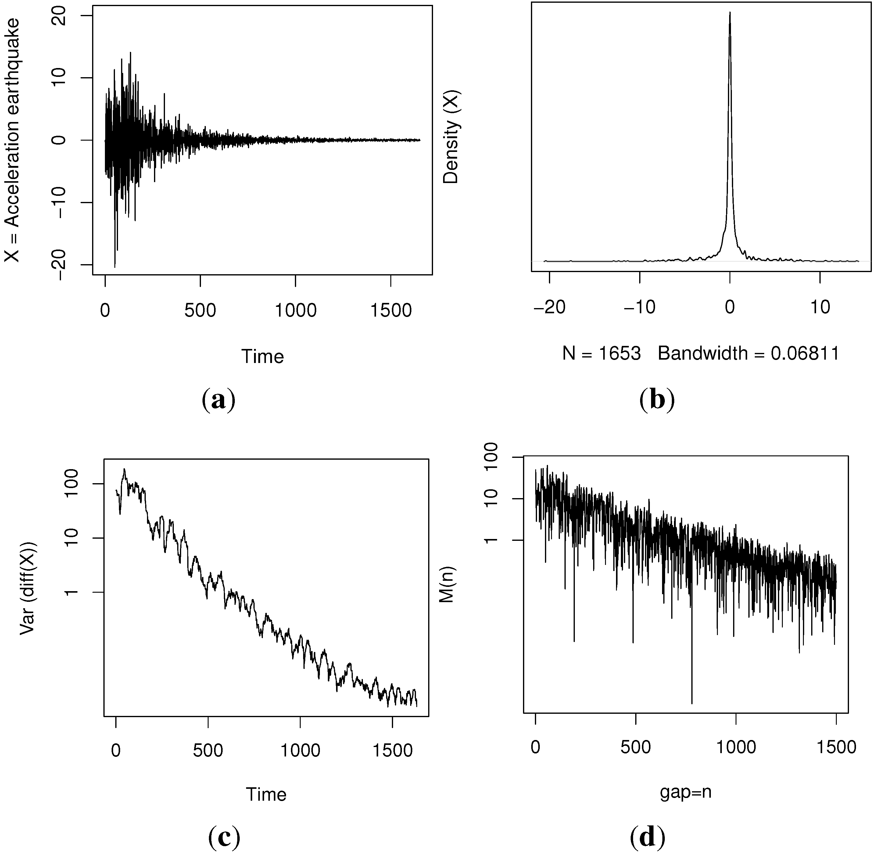
We test and validate our method through simulations and illustrate it with data from the big earthquake that occurred in Chile in 2010.
The definition of the process and some properties are presented in Section 2. In Section 3, we describe the ABC-MCMC algorithm. The simulated and real data results are shown in Section 4, and finally, in Section 5, we give some final remarks.

2. Generalized Gamma-Modulated Process

Let us consider the standard Brownian motion, { B t } t > 0 , and a Gamma process, { γ t } t > 0 , as defined in [4].
A Gamma process is a pure-jump increasing Lévy process with independent and stationary Gamma increments for non-overlapping intervals. For this process, the intensity measure is given by κ ( x ) = a x 1 exp ( b x ) , for any positive x. That is, jumps whose size lies in the interval [ x , x + d x ] occur as a Poisson process with intensity κ ( x ) d x . The parameters involved in the intensity measure are a, which controls the rate of jump arrivals, and b, the scaling parameter, which controls the jump sizes.
The marginal distribution of a Gamma process at time t is a Gamma distribution with mean a t / b and variance a t / b 2 , allowing also the parametrization in terms of the mean, μ, and variance, σ 2 , per unit time, that is, a = μ 2 / σ 2 and b = μ / σ 2 .
For the one-dimensional distributions, we have that α γ t ( a , b ) = γ t ( a , b / α ) in distribution; E ( γ t n ) = b n Γ ( a t + n ) / Γ ( a t ) , n 0 , where Γ ( z ) is the Gamma function; E ( exp ( θ γ t ) ) = ( 1 θ / b ) a t , for θ < b , and its characteristic function, ϕ γ t ( u ) = E ( exp ( i u γ t ) ) , is:
ϕ γ t ( u ) = 1 u b i a t .
Given times s < t , C o r r ( γ s , γ t ) = s / t , and given h > 0 , the density, f h ( y ) , of the increment γ t + h γ t is given by the Gamma density function with mean a h / b and variance a h / b 2 ,
f h ( y ) = y a h 1 b a h e b y Γ ( a h ) .
In this work, we will consider a = b = 1 / 2 .
Given a real value α [ 1 , 0 ] , we define the generalized Gamma-modulated (G-M) process by:
α X t = B t γ t α , f o r   t > 0 .
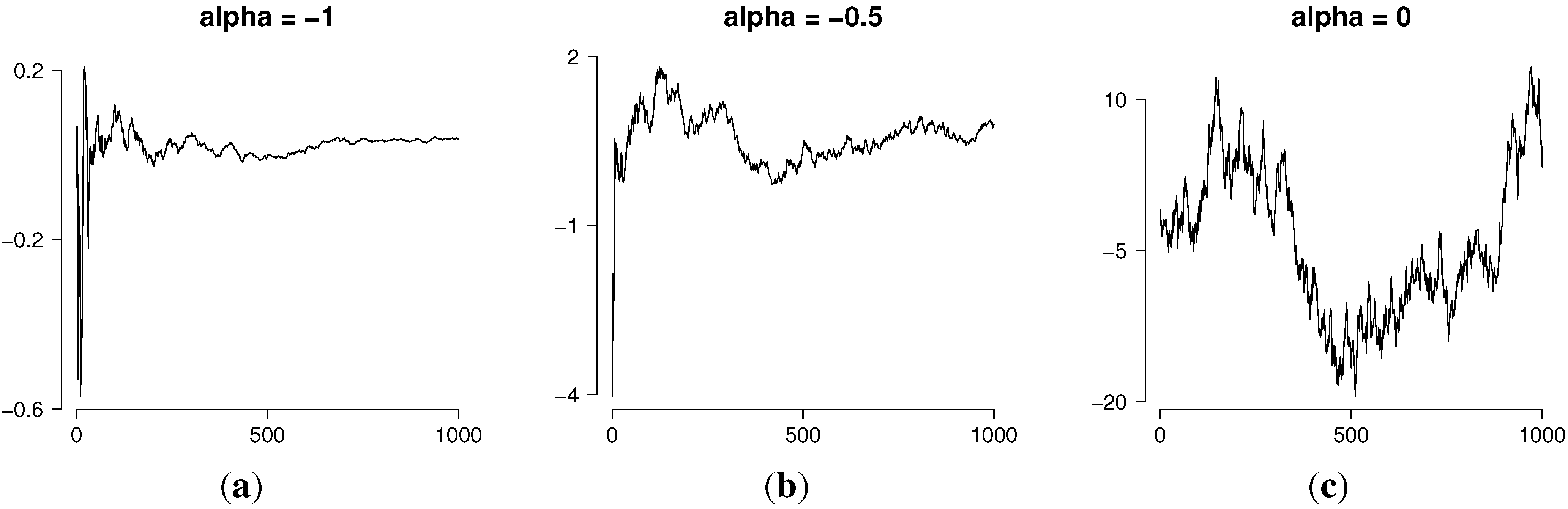
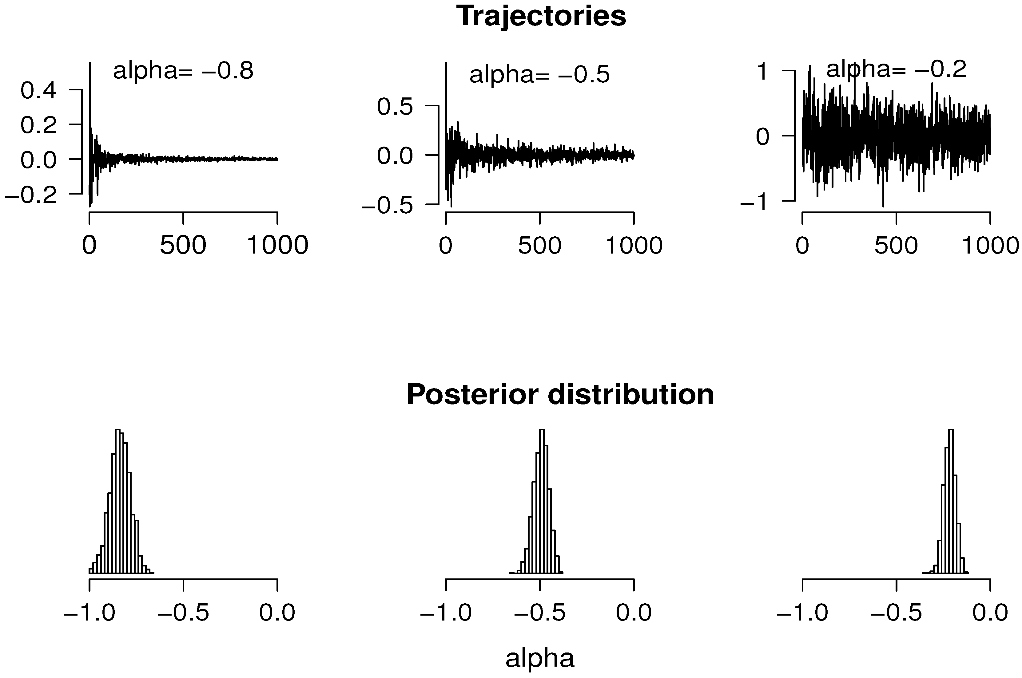
Figure 1 shows typical realizations of the generalized G-M process for different values of the parameter α. In particular, the value α = 0 corresponds to the Brownian motion and α = 0 . 5 to the Student process studied in [4].
The next subsections present some useful path characteristics of the process that could lead us to choose this model as an appropriate one for a given problem and to help us make inferences about its parameters, such as the presence of long memory, the variability profile and the variance of the increment process.
Figure 1. Realizations of the generalized Gamma-modulated (G-M) process for different values of α. (a) α = 1 ; (b) α = 0 . 5 ; (c) α = 0 .
Entropy 17 06576 g001

2.1. Explosion at Zero

The graphs in Figure 1a,b, with α < 0 , show that the process is highly variable near t = 0 , but as t , its variability decreases. We call this path property “explosion at zero” and prove it in the next result.
Proposition 1. Let α X t be the generalized Gamma-modulated process as defined in Equation (1). Then, for all M > 0 , we have:
lim s 0 P | α X s | > M = 1 , if α < 0 ; 0 , if α = 0 .
Proof. Let us consider M > 0 and α < 0 . Conditioning in γ s , we obtain:
P | B s | > M γ s α = 0 1 Γ ( s / 2 ) x s / 2 1 2 s / 2 e x / 2 P | B s | > M x α d x = 0 1 Γ ( s / 2 ) x s / 2 1 2 s / 2 e x / 2 M x α 2 e u 2 / 2 s 2 π s d u d x e A s α / 2 1 2 s / 2 0 A s α x s / 2 1 Γ ( s / 2 ) M A 2 e v 2 / 2 2 π d v d x M A e ( M A ) 2 / 2 1 + ( M A ) 2 e A s α / 2 A s / 2 s α s / 2 2 s / 2 Γ ( s / 2 ) 2 s ,
with A > 0 . The last quantity tends to one as s 0 for α < 0 .
Let us consider now the case α = 0 ,
P | B s | > M = M / s 2 e v 2 / 2 2 π d v e M 2 / 2 s s M ,
that tends to zero as s 0 .  ☐

2.2. The Increment Process

Let us now consider the increment process, Δ ( α X t ) = B t γ t α B t 1 γ t 1 α . The next results describe the asymptotic behavior of the variance-covariance structure for these differences and, hence, for the process itself, since α X t has zero expectation.
Proposition 2. For the increment process, Δ ( α X t ) ,
V a r ( Δ ( α X t ) ) t 2 α .
Proof. Let us observe that the increment process, Δ ( α X t ) = B t γ t α B t 1 γ t 1 α , can be written as Δ ( α X t ) = W t + V t , where:
W t = B t ( γ t α γ t 1 α ) , V t = ( B t B t 1 ) γ t 1 α .
Working out each term, we obtain:
V a r ( V t ) = E ( ( B t B t 1 ) 2 γ t 1 2 α ) = E ( γ t 1 2 α ) t 2 α ,
V a r ( W t ) = E ( B t 2 ( γ t α γ t 1 α ) 2 ) = t E ( ( γ t α γ t 1 α ) 2 ) t 2 α 1 ,
and:
C o v ( V t , W t ) ( t 1 ) α ( t α ( t 1 ) α ) t 2 α 1 .
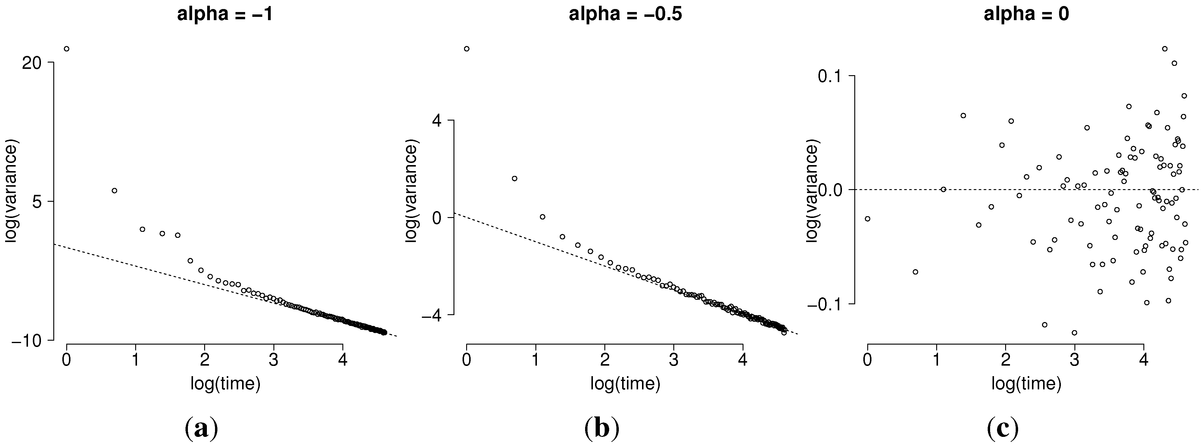
This property leads us to consider the variance of the observed increment process, V a r ( Δ ( α X t ) ) t 2 α , as informative for the parameter α and, therefore, helpful to implement the approximated simulation for its marginal posterior.
In a data exploratory phase, we could examine the graph of the empirical variances of Δ ( α X t ) from t to the end of the process, as a function of t in logarithmic scale. As t increases, that graph should become linear with slope 2 α . Figure 2 exhibit this result for some values of α. Observe that the asymptotic result can be visualized from log t 3 , that is from t 20 , for α < 0 .
Figure 2. Sample distribution of V a r ( Δ ( α X t ) ) , for 1000 simulated trajectories of the generalized G-M process, for different values of α. (a) α = 1 ; (b) α = 0 . 5 ; (c) α = 0 .
Entropy 17 06576 g002
Proposition 3. The auto-covariance for lag n of the increment process, denoted by M α ( n ) , is of order n α 1 , if 1 < α < 0 , and it is zero, if α = 0 , as n increases.
Proof. Let us consider n 3 , because of the explosion at zero. Then:
M α ( n ) = E ( Δ ( α X 3 ) Δ ( α X n + 3 ) ) M α ( n ) = E ( ( B 3 γ 3 α B 2 γ 2 α ) ( B n + 3 γ n + 3 α B n + 2 γ n + 2 α ) ) = E ( B 3 γ 3 α B n + 3 γ n + 3 α ) E ( B 3 γ 3 α B n + 2 γ n + 2 α ) E ( B 2 γ 2 α B n + 3 γ n + 3 α ) + E ( B 2 γ 2 α B n + 2 γ n + 2 α ) = E ( B 3 B n + 3 ) E ( γ 3 α γ n + 3 α ) E ( B 3 B n + 2 ) E ( γ 3 α γ n + 2 α ) E ( B 2 B n + 3 ) E ( γ 2 α γ n + 3 α ) + E ( B 2 B n + 2 ) E ( γ 2 α γ n + 2 α ) = 3 E ( γ 3 α γ n + 3 α γ 3 α γ n + 2 α ) 2 E ( γ 2 α γ n + 3 α γ 2 α γ n + 2 α ) .
Observe that:
E ( γ t α γ s α ) = 1 2 t / 2 1 Γ ( ( t s ) / 2 ) Γ ( s / 2 ) 0 0 γ t γ t α γ s α + s / 2 1 ( γ t γ s ) ( t s ) / 2 1 e γ t / 2 d γ s d γ t = 1 2 t / 2 1 Γ ( t s 2 ) Γ ( s / 2 ) 0 0 γ t γ s α ( γ t γ s ) ( t s ) / 2 1 γ s s / 2 1 d γ s γ t α e γ t / 2 d γ t = 1 2 t / 2 1 Γ ( t s 2 ) Γ ( s / 2 ) 0 0 1 z α + s / 2 1 ( 1 z ) ( t s ) / 2 1 d z γ t 2 α + t / 2 1 e γ t / 2 d γ t = 1 2 t / 2 1 Γ ( t s 2 ) Γ ( s / 2 ) Γ ( α + s / 2 ) Γ ( ( t s ) / 2 ) Γ ( α + t / 2 ) 0 γ t 2 α + t / 2 1 e γ t / 2 d γ t = 1 2 t / 2 1 Γ ( t s 2 ) Γ ( s / 2 ) Γ ( α + s / 2 ) Γ ( ( t s ) / 2 ) Γ ( α + t / 2 ) Γ ( t / 2 + 2 α ) ( 1 / 2 ) t / 2 + 2 α = 4 α Γ ( α + s / 2 ) Γ ( 2 α + t / 2 ) Γ ( s / 2 ) Γ ( α + t / 2 ) .
If 1 < α < 0 , we can apply the Gautschi inequality [12], obtaining:
E ( γ t α γ s α ) ( s t ) α ,
and then:
M α ( n ) = E ( γ 1 α γ n + 1 α ) E ( γ 1 α γ n α ) ) n α 1 .
On the other hand, for α = 0 , E ( γ t α γ s α ) = 1 , and therefore, M 0 ( n ) = 0 .  ☐
In other words, for α = 0 , the process has no memory, and we recover the Brownian motion case as already mentioned; for α < 0 , the process is called anti-persistent. Recalling the Hurst parameter H associated with the fractional Brownian motion, the relationship between H and α is α = 2 H 1 ; see [4], for instance.

3. ABC-MCMC Study

When dealing with non-standard posterior distributions, the usual procedure is to use Markov chain Monte Carlo simulation to produce an approximate sample from this posterior. However, when the likelihood function is intractable, MCMC methods cannot be implemented. The class of likelihood-free methods termed, approximate Bayesian computation (ABC), can deal with this problem as long as we are able to simulate from the probabilistic model and a suitable set of summary statistics is available.
The ABC idea was proposed by Pritchard et al. [13] and developed further in the last decade. In particular, with respect to the choice of the summary statistics from among diverse options, in [14], the authors consider a sequential test procedure for deciding whether the inclusion of a new statistic improves the estimation. In [15], the discussion refers to the choice of informative statistics related to the algorithmic properties.
In our case, in order to perform the ABC algorithm for the memory parameter, α, we have to be able to generate a realization of the target process and we have to know which are the important observable characteristics of the process that lead us to increase our information about α.
Observe that we already know, by Equation (1), how to simulate from the generalized G-M for each value of the parameter. After obtaining a simulated trajectory, we can compare it then to the observed trajectory through adequate statistics. Intuitively, if they are similar enough, the chosen value of the parameter can be thought of as an appropriate one.
More concretely, suppose that we take the observed increments d t = Δ ( x t ) from a sample x t and that for each α [ 1 , 0 ] , we generate a realization from a Brownian motion b t and a realization from a Gamma process γ t , obtaining:
Δ ( α x t ) = b t γ t α b t 1 γ t 1 α .
For the ease of notation, set α y t = Δ ( α x t ) . To compute the proximity between d t and α y t , we will determine the distance between some statistics for each sample. The usual choices for the memory parameter are, among others, the rescaled range R / S or the rescaled variance V / S , the periodogram, quadratic variations, aggregated variances, Whittle estimator and functions, as the logarithm, inverse or square root, of these ones [15,16]. In [7], we used those statistics to obtain approximate posterior samples for the memory parameter for fractional self-similar processes.
We tried all of them in this work; however, their performance was not good enough, because of the non-stationarity and the inherent heteroscedasticity of the process. To solve this situation, we considered the slope of the regression of the sampling variance of m-size blocks on the time, regarding the results in Section 2.2, and this solution worked much better than the former ones.
Let T * denote the following statistic. Giving n observations and an integer m < < n , we take consecutive blocks of size m and obtain the sampling variance for each block, s 2 ( k ) , for k = 1 , , n / m , where ξ is the integer part of ξ. Those values are used as estimates for the variances at times m , 2 m , , n / m m . In log log scale, the slope of the regression line obtained through the points ( k m , s 2 ( k ) ) , k = 1 , , n / m , should be of order of 2 α , as time increases. We define T * as this slope.
The ABC steps for α are then given by the following algorithm.
Algorithm 1 ABC procedure for α.
  • Select α from a prior distribution π ( α ) U n i f [ 1 , 0 ] ;
  • Generate a trajectory α y t for that value α;
  • Given ε > 0 , if | T * ( x t ) T * ( α y t ) | < ε , then select α for the sample S α , otherwise, reject it;
  • Repeat Steps 1–3 until reaching an adequate sample size for the parameter α.
The sample S α obtained in the last step is an approximate sample from the posterior distribution for α, the goodness of which strongly depends on the choice of the statistics and the threshold ε in Step 3.
Note that if ε is too small, then the rejection rate is high, and the algorithm becomes too slow; on the other hand, if ε is too big, the algorithm accepts too many values of α, giving a less precise approximate sample. In general, what is done is to take a small percentile of the simulated distances, that is we select those α’s giving the closest values to the observed one. In this work, after some trial, we used the first percentile, as proposed by [17].
Let us consider now the more general model for the increments given by:
Y t = μ + 1 τ Δ ( α X t ) ,
for μ , τ R and τ > 0 , representing the precision of the fluctuations. As: Δ ( α X t ) = B t γ t α B t 1 γ t 1 α , with B t B t 1 N ( 0 , 1 ) , γ t γ t 1 χ 2 ( 1 ) and B t independent of γ t , for all t > 0 , and following the theory associated with the Gamma-modulated process [4], it is possible to assume a hierarchical representation.
We can rewrite the above model in a multivariate way as:
( Y 1 , , Y n ) μ , τ , γ , α N μ 1 , τ 1 Σ ( γ , α ) ,
where, for i , j = 1 , , n ,
Σ i i = i γ i α γ i + 1 α 2 + γ i + 1 2 α , Σ i j = γ j α γ j + 1 α i γ i α ( i + 1 ) γ i + 1 α , f o r   i < j .
As a final step, let us assume prior distributions given by:
μ τ N ( b 0 , g ( τ ) v 0 ) τ Γ ( a 0 , d 0 ) ,
and prior knowledge for α, π ( α ) . Then, given 0 < γ 1 < γ 2 < < γ n + 1 , auxiliary random effects distributed as:
π ( γ 1 , , γ n ) i = 1 n + 1 ( γ i γ i 1 ) 1 / 2 e γ n + 1 / 2 ,
and an observed trajectory y = ( y 1 , , y n ) , the posterior distribution can be computed from:
π ( μ , τ , γ 1 , , γ n , α y ) π ( γ 1 , , γ n ) π ( τ ) π ( α ) τ n / 2 Σ ( γ , α ) 1 / 2 × exp τ 2 ( y μ 1 ) Σ ( γ , α ) 1 ( y μ 1 ) .
After straightforward computations and assuming that g ( τ ) = 1 , the full conditional posterior distributions for μ , τ are:
μ y , τ , γ 1 , , γ n , α N b 1 , v 1 ,
τ y , μ , γ 1 , , γ n , α Γ a 1 , d 1 ,
where:
b 1 = v 0 + τ 1 Σ ( γ , α ) 1 1 1 τ 1 Σ ( γ , α ) 1 y + v 0 b 0 , v 1 = v 0 + τ 1 Σ ( γ , α ) 1 1 ,
a 1 = n / 2 + a 0 , d 1 = d 0 + 0 . 5 ( y μ 1 ) Σ ( γ , α ) 1 ( y μ 1 ) .
With this notation, for parameters ( μ , τ , α ) , we propose the following ABC-MCMC procedure.
Algorithm 2 ABC-MCMC procedure for ( μ , τ , α ) .
  • Apply the ABC proposal given by Algorithm 1, to obtain a posterior sample for α, S α ;
  • Sample uniformly from α S α ;
  • Generate a trajectory γ = ( γ 1 , , γ n ) from the Gamma process;
  • Sample ( μ , τ ) from the conditional posterior π ( μ , τ α , γ , y ) ;
  • Repeat Steps 3–4 until the convergence is reached, which can be checked by the usual graphical criterion for ( μ , τ ) , and take their sampling mean;
  • Repeat Steps 2–5, for obtaining a complete posterior sample for ( μ , τ , α ) .
The whole procedure is to then use the ABC algorithm for α and the MCMC scheme for μ , τ to perform the Bayesian inference of our proposal.

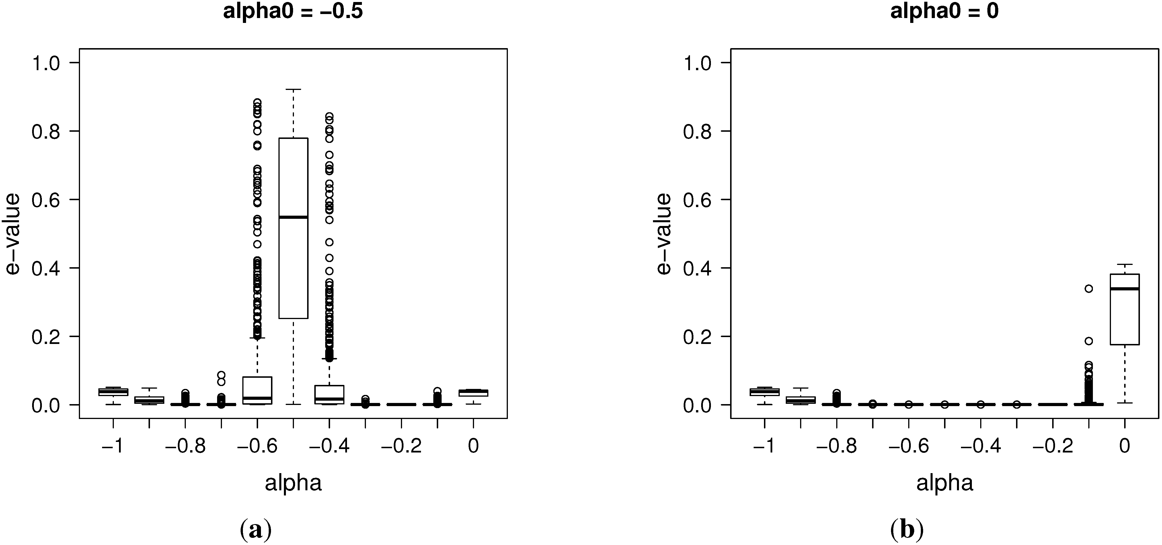
3.1. Posterior Evidence for Sharp Hypotheses

As a by-product of the previous algorithm, we are able to compute approximately the so-called e-value, an evidence measure defined in [8] for precise hypothesis testing, which we describe briefly below.
Let us consider a hypothesis of interest H : α Ω 0 , and define the tangential set T 0 to Ω 0 as the set:
T 0 = { ( μ , τ , α ) Ω : π ( μ , τ , α y ) > π 0 } , w h e r e   π 0 = sup Ω 0 π ( μ , τ , α y ) .
In other words, the tangential set to Ω 0 considers all points “more probable” than those in Ω 0 , according to the posterior law.
The evidence measure e-value for the hypothesis H is defined as:
e v ( Ω 0 ) = 1 T 0 π ( μ , τ , α y ) d μ d τ d α .
Therefore, if the tangential set has high posterior probability, the evidence in favor of H is small; if it has low posterior probability, the evidence against H is small. For instance, suppose that we are considering the sharp hypothesis H : α = α 0 . If the subset α = α 0 has high density, that is it lies near the mode of π ( μ , τ , α y ) ), then the e-value must be large, giving high evidence for that sharp hypothesis. Some interesting hypotheses are the precise ones defining the Brownian motion case, when α = 0 , and the G-M process, when α = 0 . 5 .
In this work, we approximate empirically the integral in the e-value using the posterior sample obtained by the previous algorithms. As usual, in the Bayesian paradigm, the predictive distribution for the next steps can be computed using this ABC-MCMC sample and the model Equation (2).

4. Numerical Results

In this section, we present the main results after implementing our algorithms in the R-gui software [18], using simulated and real data. Hence, we will show the performance of our proposal and its use in practice.

4.1. Simulated Results

To illustrate the performance of our procedure, we simulate 500 replicates of length n = 1000 , for a grid with α [ 1 , 0 ] by 0 . 1 , when μ = 0 and τ = 1 are fixed.
Figure 3 shows three trajectories for α = 0 . 8 , 0 . 5 , 0 . 2 and their respective approximate posterior densities obtained by Algorithm 1, with posterior means (and 95 % credible intervals) 0 . 835 ( 0 . 939 , 0 . 735 ) , 0 . 495 ( 0 . 579 , 0 . 421 ) , 0 . 217 ( 0 . 278 , 0 . 157 ) .
Figure 3. Realizations of the increments of the generalized Gamma-modulated process for different values of α and the posterior density obtained by the approximate Bayesian computation (ABC) algorithm for α.
Entropy 17 06576 g003
In Figure 4, we see the sampling distribution of the posterior mean for α. Observe that the estimates we obtained are fairly precise for all values in the interval [ 1 , 0 ] .
In order to confirm that precision, we obtained the e-values associated with the hypothesis α 0 = 0 . 5 , when the nominal value for α varies in [ 1 , 0 ] , as shown in Figure 5a. The boxplots show the sampling distribution for these e-values from the 500 replicates for each α { 1 , 0 . 9 , , 0 . 1 , 0 } . Observe that the obtained e-values are coherent with the previous estimates, giving high evidence to α 0 = 0 . 5 when the nominal value is close to it and low evidence otherwise.
Figure 4. Sampling distribution of the posterior mean for α.
Entropy 17 06576 g004
Figure 5. Sampling distribution of the e-value for: (a) α 0 = 0 . 5 ; (b) α 0 = 0 .
Entropy 17 06576 g005
In the case α 0 = 0 , shown in Figure 5b, even when the e-value is not as high for α = 0 as in the previous case, it does allow for a good discrimination in favor of the null hypothesis.
In the general case, when μ and τ are unknown, we applied Algorithm 2, reporting the following results for the nominal values μ = 10 and τ = 1 , as illustrated in Figure 6. The numerical results were very similar for other values in terms of precision and computational time.
It is worth noting the symmetry of the sampling distribution of the posterior mean for μ, as well as the asymmetry of the sampling distribution of the posterior mean for τ, as it was supposed to be by Equation (3). Furthermore, the estimates are consistent around the nominal value.
Figure 6. Sampling distribution of the posterior mean for: (a) μ; (b) τ.
Entropy 17 06576 g006
The results suggest that, as α 1 , the data become more informative for the location parameter. Inversely, for the precision parameter τ, the estimates seem to be less accurate as α goes to 1 . Both features are related to the behavior of the trajectories: as α decreases to 1 , the increments stabilize faster around zero than for α closer to zero, and consequently, we obtain more precise estimates for μ. This very behavior explains the posterior for τ: the fast stabilization of the increments leads to underestimating the variance, that is to overestimating the precision. The same results were observed for other nominal values of μ and τ.

4.2. Earthquake Acceleration Data

Our proposal is illustrated extending the ideas in [4]. We analyze sequential data obtained from an accelerometer recording the big earthquake in Southern Chile (27 February 2010), with the epicenter in Cobquecura, approximately 335 km southwest of Santiago, which reached 8.8 on the Richter scale. The dataset was obtained from the Hydrographic and Oceanographic Service of the Chilean Navy. The time series was recorded at a rate of 50 observations per second, with n = 1653 , as shown in Figure 7a.
A brief exploratory analysis of the data, summarized in Figure 7b–d, led us to believe that the proposed model can be well fitted according to the properties described in Section 2.
The marginals for the posterior distribution are shown in Figure 8, with posterior means for the parameters equal to α ˰ = 0.975 ( ± 0 . 021 ) , μ ˰ = 0 . 0007 ( ± 0 . 007 ) , τ ^ = 106305 ( ± 3800 ) . Observe, in the first scatterplot, the sharp and negative posterior correlation between α and τ, as expected by Equation (3). Furthermore, the e-values for the hypotheses α 0 = 0 . 5 and α 0 = 0 are clearly zero, as confirmed by both graphs.
Figure 7. (a) Acceleration earthquake series, X t ( n = 1653 at 50 observations per second) and exploratory graphics: (b) density of the raw data; (c) sample variance of the increment process, V a r ( Δ ( X t ) ) , in log-scale; (d) sample auto-covariance, M ( n ) , in log-scale.
Entropy 17 06576 g007
Figure 8. Marginal posterior distributions for the parameters in the acceleration earthquake series.
Entropy 17 06576 g008

5. Final Remarks

The model proposed here seems to be suitable for the phenomena under study. In particular, interesting properties, including long memory and trajectory behavior, are discussed, on which our inference methodology is grounded.
For the ABC algorithm, we considered at first a minimum entropy criterion for selecting the approximate posterior sample, because that choice had a good performance in estimating the long memory parameter for stationary non-Gaussian processes as, for instance, binary and the Rosenblatt processes [7]. However, given the trajectory behavior of the G-M process, the most informative statistics we found is the m-block variance statistic T * .
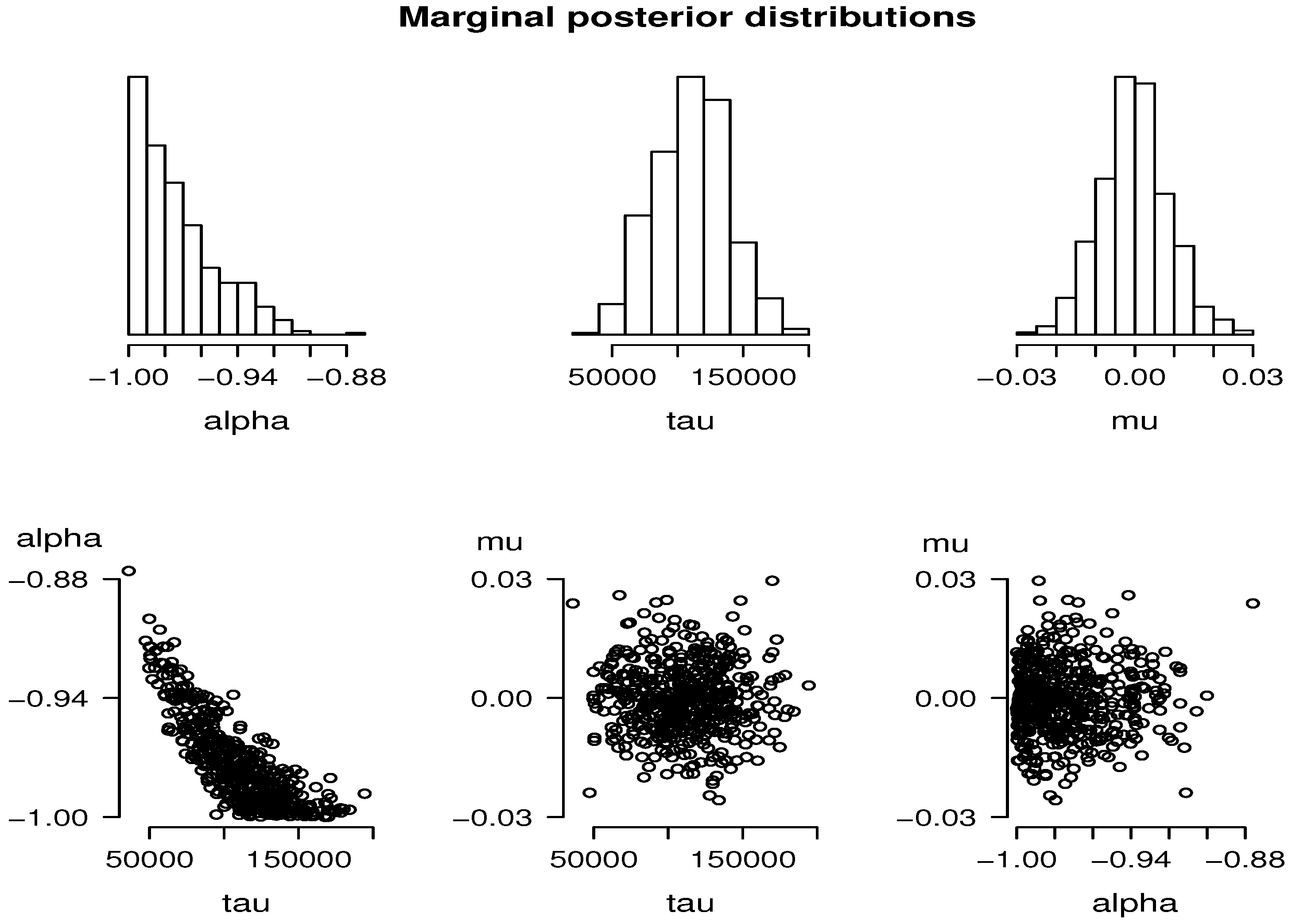
Our results show, firstly, a clear and easy way of implementing the ABC-MCMC algorithms in a standard software. For the real data ( n = 1653 ), the computational cost was moderate, obtaining a posterior sample of a size of 500 from the ABC-MCMC proposal in one hour.
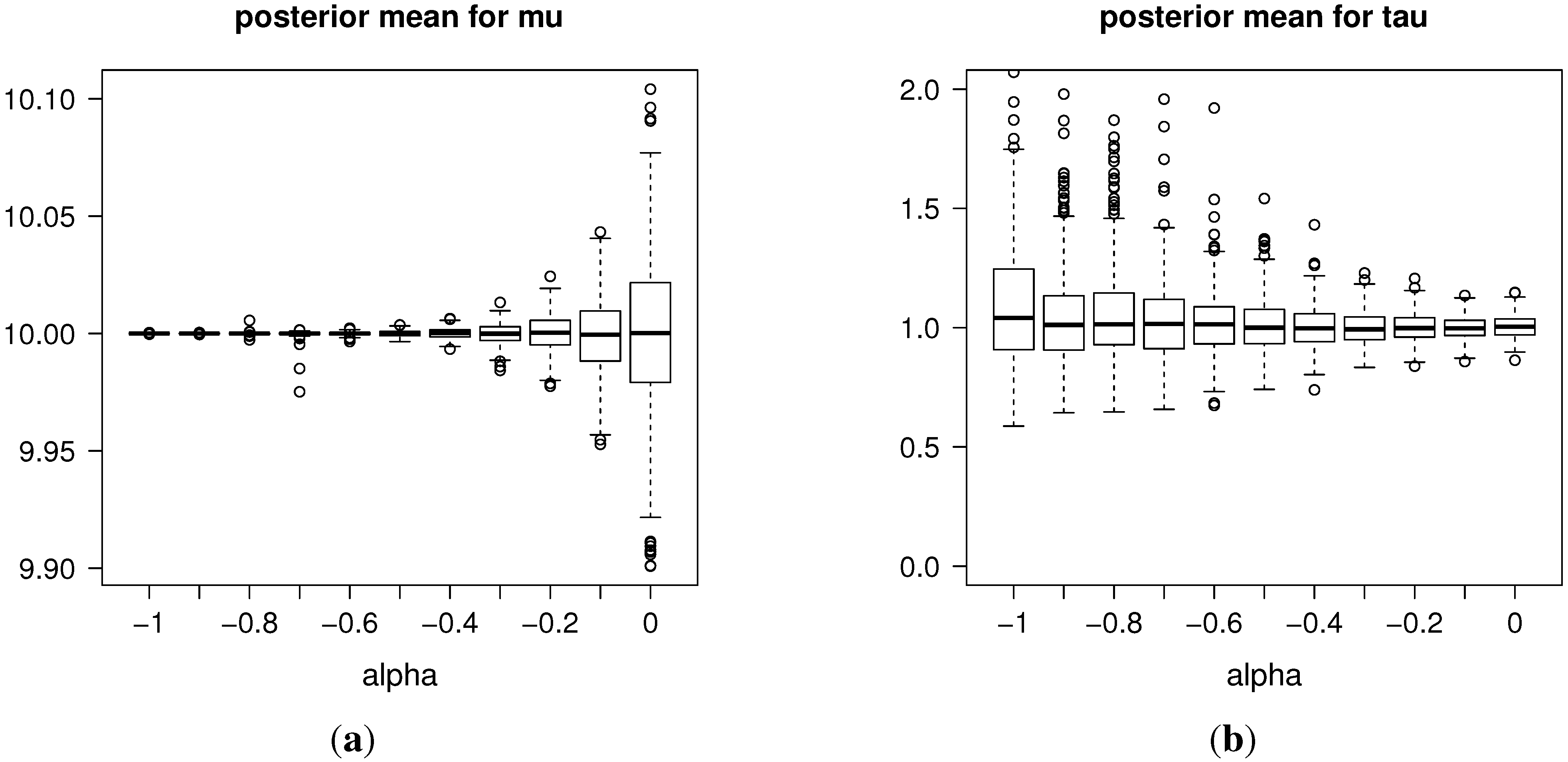
In our simulations, we obtained a very high precision in the estimates given by this procedure. In addition, the estimates for the precision parameter, τ, are affected reasonably by scale changes. For instance, for the rescaled data, z = c × y , we estimated τ as τ * = τ ^ / c 2 , approximately.
The chosen parameterization allows for α ( 0 , 1 ] . However, we did not study such a case, since that process diverges as time increases, making the inference procedure harder for α. We recommend then to treat this problem as a separate case.
Finally, we believe that this model has wider applications, mainly for its parsimony and the straightforward interpretation of the parameters. For diagnostic purposes, for example, the predictive series could be used to perceive the increasing fore-shocks before the arrival of a new earthquake.

Acknowledgments

Andrade is a PhD student with CNPq Grant No. 141048/2013-1 at the University of São Paulo. Rifo and Torres-Avilés were partially supported by the program Escala Docente Asociación de Universidades Grupo Montevideo 2014 between University of Campinas and Universidad de Santiago de Chile. Torres was partially supported by the Project PROGRAMA INVESTIGACIÓN ASOCIATIVA CONICYT Cuarto Concurso Nacional de Anillos de Investigación en Ciencia y Tecnología 2011, Red de Análisis Estocástico y Aplicaciones (sistemas abiertos, energía y dinámica de la información) ACT 1112 and Fondecyt Grant 1130586. This work was also developed as part of Inria Chile under project “Communication and information research & innovation center”, 10CEII-9157. Torres-Avilés was partially funded by Fondecyt 11110119. For Rifo, this article was produced as part of the activities of FAPESP Center for Neuromathematics, Grant No. 2013/ 07699-0, São Paulo Research Foundation.

Author Contributions

All of the authors developed the model and the methodology presented in this paper. Plinio Andrade performed the simulations and data analysis and wrote the paper. All of the authors have read and approved the final manuscript.

Conflicts of Interest

The authors declare no conflict of interest.

Appendix: Discussion of Other Models

Let us consider a complete filtered probability space ( Ω , F , P ; { F t } ) that supports a Brownian motion, { B t } , a positive random variable, W, and a Gamma process { γ t } with parameters α = 1 / 2 , β = 2 . Suppose that all of the processes are adapted to the filtration { F t } and are mutually independent. Furthermore, assume that { F t } is the right continuous filtration associated with ( B , W , γ ) .
Consider the following three processes defined by:
  • ξ t = B t ;
  • T t = B t / W , where W is a positive random variable and;
  • T t = B t + 1 γ t + 1 1 / 2 .
The increment of the process { ξ t } defines a random i.i.d. noise with a Gaussian distribution, representing the most common noise used in the literature for regression models. The increments of the second noise describe a perturbation of a Gaussian i.i.d. error in the distributional sense. This process will be called t-homoscedastic, given that the increments remain independent and with the same distribution, whose variance is related to the degrees of freedom of the independent variable W. Specifically, we are interested in the case where W is a χ 2 random variable with ν degrees of freedom.
Finally, the third noise is the Gamma-modulated process, as defined in [4].

A. Some Properties of the Models

A.1. Heteroscedastic t-Student Process

Proposition 4. The one-dimensional densities of T t , Δ T t = T t T s and ( Δ T t , T s ) for fixed 1 < s < t are given by:
f T t ( x ) = 0 ϕ x ; 0 , t γ d Γ t ( γ ) ,
f Δ T t ( x ) = ϕ x ; 0 , g ( γ 1 , γ 2 ) d Γ t s ( γ 1 ) d Γ s ( γ 2 ) ,
f ( Δ T t , T t ) ( x ¯ ) = ϕ x ¯ ; 0 , Σ d Γ t s ( γ 1 ) d Γ s ( γ 2 ) ,
where Γ t is the cdf of γ t , ϕ ( x ; μ , σ 2 ) denote the univariate density at x of a normal distribution with mean μ and variance σ 2 ,
g ( γ 1 , γ 2 ) = s 1 γ 2 1 γ 1 + γ 2 2 + t s γ 1 + γ 2 ,
and
Σ = t s γ 1 + s 1 γ 1 γ 2 2 s γ 2 1 γ 1 γ 2 s γ 2 1 γ 1 γ 2 s γ 2 .
Proof. The densities are consequences of standard computation. ☐

A.2. Homoscedastic t-Student Process

Proposition 5. The homoscedastic t-Student process is conditionally independent and has stationary increments. Furthermore,
E ( T t ) = 0 , E ( T t 2 ) = t E ( W 1 ) , i f   E ( W 1 ) < , E ( T t k ) = t k / 2 E ( Z k ) E ( W k / 2 ) , i f   E ( W 1 / 2 ) < ,
where Zis a standard Gaussian random variable with E ( Z k ) = 0 , if k is odd, and E ( Z k ) = 2 k / 2 Γ k + 1 2 / π , if k is even.
Additionally, for s < t , the covariance is given by:
E ( T t T s ) = s E ( W 1 ) .
Finally, for given t, the density of T t is:
f T t ( x ) = 0 N ( x ; 0 , t / W ) d F W ( w ) .
Proof. The proof is a consequence of algebraic calculations.  ☐

B. Diffusion Models

In this section, we will consider the Euler discretization of the linear stochastic differential equation:
d Y t = μ d t + σ d E t ,
where the noise E t has one of the following characteristics:
  • standard Brownian motion or Gaussian noise;
  • homoscedastic t-Student noise or;
  • Gamma-modulated process withheteroscedastic t-Student noise.
Then, the discrete version of Equation (5) is given by y i = μ Δ ( t ) + σ Δ E t . In each case, the discretization of the errors can be represented as a combination of the scale and location parameters in a Gaussian model.

B.1. Linear SDE with Gaussian Independent Errors

In this section, we will consider the following discretized model of Equation (5), when the noise is given by the increment of a Brownian motion. In this case, y i , 1 i n , is a discrete version of Equation (5), with ( Δ = 1 ) given by:
y i = μ + σ ( B i + 1 B i ) ,
for i = 1 , , n . We will assume that ( μ , σ 2 ) is independent of { B t } t 0 . Under this framework, the conditional setting is given by:
y μ , σ 2 , Σ N n ( μ X , σ 2 Σ ) ,
where Σ = I n , X = 1 n is the n-dimensional vector of ones, and μ = β .
Considering the following prior specification:
μ σ 2 N ( b 0 , τ 0 2 ) σ 2 I G ( a 0 , d 0 ) ,
where B 0 = τ 0 2 and b 0 , a 0 , d 0 and τ 0 2 are known, then it is straightforward to obtain the complete conditional distributions. To approximate the posterior distributions, we need to sample from:
μ σ 2 , y N ( m , τ 2 ) σ 2 μ , y I G ( a , d ) ,
where m = ( σ 2 b 0 + τ 0 2 y ¯ n ) / ( σ 2 + n τ 0 2 ) , τ 2 = σ 2 τ 0 2 / ( σ 2 + n τ 0 2 ) , a = n 2 + a 0 and d = 1 2 i = 1 n ( y i μ ) 2 + d 0 .

B.2. Linear SDE with t-Student Homoscedastic Errors

In this model, we will consider fixed t-Student distributed errors, which means that we will contaminate the noise with a fixed χ 2 random variable with ν degrees of freedom. In this model, the increments have a t-Student distribution with the same degrees of freedom, that is the increments are stationary. Then, the discretized version of the t-Student homoscedastic model for the SDE Equation (5), with Δ = 1 , is given by:
y i = μ + W 1 / 2 σ ( B i + 1 B i ) ,
for i = 1 , , n , W I G ( ν / 2 , ν / 2 ) , that is if G = W 1 , then f G ( g ) = ( ν / 2 ) ν / 2 Γ ( ν / 2 ) g ν / 2 1 e g / 2 for w 0 ; and W is independent of { B t } t 0 . We will also assume that the vector ( μ , σ 2 ) is independent of W , { B t } t 0 . As before, we adopt the conditional setting:
y μ , σ 2 , ω N n ( μ , ω σ 2 I n ) , ω I G ( ν / 2 , ν / 2 ) ,
and
( μ , σ 2 ) ω .
It is straightforward to prove that if we integrate out W, we obtain:
y μ , σ 2 t n ( μ 1 n , σ 2 I n , ν ) ,
where t n ( μ , Σ , ν ) denote the n-dimensional t distribution.
Thus, if we consider:
μ σ 2 N ( b 0 , g ( σ 2 ) B 0 ) , σ 2 I G ( a 0 , d 0 ) ,
and put Σ = ω I n , with ω I G ( ν / 2 , ν / 2 ) , g ( σ 2 ) = 1 , B 0 = τ 0 2 and X = 1 n , we obtain:
μ σ 2 , ω , y N ( m , τ 2 ) σ 2 μ , ω , y I G ( a , d ) ω μ , σ 2 , y I G ( a 1 , d 1 ) ,
where m = ( σ 2 b 0 w + y ¯ τ 0 2 ) / ( w σ 2 + τ 0 2 n ) , τ 2 = σ 2 w τ 0 2 / ( w σ 2 + τ 2 n ) , a = n 2 + a 0 , d = i = 1 n ( y i μ ) 2 / ( 2 w ) + d 0 , a 1 = ( ν + n ) / 2 and d 1 = i = 1 n ( y i μ ) 2 / ( σ 2 ) + ν / 2 .

B.3. Gamma Modulated Process-t-Student Heteroscedastic Model

In this case, the discrete version of the process has the following representation:
y i = μ + σ B i + 1 γ i + 1 B i γ i ,
for i = 1 , , n . Again, we assume ( μ , σ 2 ) independent of { B t } t 0 , { γ t } t 0 and the prior distribution of ( μ , σ 2 ) specified as before. Hence, the model is reduced to:
y μ , σ 2 , γ N ( μ 1 n , σ 2 Σ ( γ ) ) ,
where γ is a gamma process with parameters α = β = 1 / 2 , Σ ( γ ) = A ( γ ) Λ A ( γ ) t , Λ is the covariance matrix of B = ( B 1 , , B n + 1 ) given by λ i , j = i j and A ( γ ) is the n × ( n + 1 ) matrix given by:
a i j = γ i 1 / 2 i f i = j , γ i + 1 1 / 2 i f j = i + 1 , 0 o t h e r w i s e .
Simple computation gives:
Σ i i = i 1 γ i 1 γ i + 1 2 + 1 γ i + 1 , Σ i j = 1 γ j 1 γ j + 1 i γ i i + 1 γ i + 1 f o r i < j .
On the other hand, the distribution of γ is computed from the fact that ( γ 1 , γ 2 γ 1 , , γ n + 1 γ n ) are independent χ 1 2 . Let T = t i j the matrix defined by:
t i j = 1 , i f i j 0 , o t h e r w i s e .
Then:
γ 1 γ 2 γ n = T γ 1 γ 2 γ 1 γ n γ n 1 .
By the independence of the increments, we obtain that the density of γ is proportional to:
i = 1 n + 1 ( γ i γ i 1 ) 1 / 2 e γ n + 1 / 2 , 0 < γ 1 < γ 2 < < γ n + 1 ,
where we are assuming γ 0 = 0 . Hence, Model (7) can be specified as follows:
y μ , σ 2 , γ N ( μ 1 n , σ 2 Σ ( γ ) ) , μ σ 2 , γ N ( b 0 , g ( σ 2 ) B 0 ) , σ 2 I G ( a 0 , d 0 ) , μ σ 2 , ( γ 1 , , γ n + 1 ) ( μ , σ 2 ) .
The distribution of Σ can be obtained running the Gibbs sampling on y , μ , σ 2 and γ. Usual calculations give the posterior distribution of ( μ , σ 2 ) .
In this way, the conditional distributions needed to implement the Gibbs sampling are obtained as usual by taking X = 1 n , β = μ , g ( σ 2 ) = 1 , B 0 = ν 0 2 and Σ = Σ ( γ ) , such that:
μ σ 2 , γ , y N ( m , τ 2 ) , σ 2 μ , γ , y I G ( a , d ) ,
where:
m = σ ν 0 2 + i , j Γ i , j 1 × σ ν 0 2 b 0 + i j Γ i , j y i ,
Γ = Σ 1 is a n × n matrix,
τ 2 = σ 2 σ ν 0 2 + i , j Γ i , j 1 ,
a = ( n / 2 + a 0 + 1 ) , and d = 1 2 ( y μ ) t Σ 1 ( y μ ) + d 0 .
Finally, the posterior distribution for the random vector γ = ( γ 1 , , γ n + 1 ) given μ , σ 2 , y = ( y 1 , , y n ) , such that 0 < γ 1 < γ 2 < < γ n + 1 , is:
γ μ , σ 2 , y i = 1 n + 1 ( γ i γ i 1 ) 1 / 2 e γ n + 1 / 2 σ n | Σ n / 2 | e x p ( ( γ μ ) t σ 1 Σ 1 ( γ ) ( γ μ ) ) .

C. Comparing the Models

In this section, we present two models in order to make a comparison between our proposal and other noises.

C.1. Mixed Brownian Model

Consider the processes defined by T t = B t / W , where W is a positive random variable and B is a standard Brownian motion. It has stationary increments, and:
E ( T t ) = 0 , E ( T t 2 ) = t E ( W 1 ) , i f E ( W 1 ) < , E ( T t k ) = t k / 2 E ( Z k ) E ( W k / 2 ) , i f E ( W 1 / 2 ) < ,
where Z is a standard Gaussian random variable with E ( Z k ) = 0 , if k is odd, and E ( Z k ) = ( 2 k / 2 Γ k + 1 2 / π , if k is even.
Additionally, for s < t , the covariance is given by:
E ( T t T s ) = s E ( W 1 ) .
Finally, given t > 0 , the density of T t is:
f T t ( x ) = 0 N ( x ; 0 , t / W ) d F W ( w ) .
If W = 1 almost sure, we can recover the case of the Brownian motion. Let us consider the following increments process:
T t α = ( T t T t 1 ) t α .
This process has independent increments, but is not stationary. The first two moments of the process are E ( T t α ) = 0 , V ( T t α ) = t 2 α .
The covariance structure is given by:
C O V ( T t α , T s α ) = E ( T t α T s α ) = ( s t ) α E ( ( T t α T t 1 α ) ( T s α T s 1 α ) ) = 0 .
and finally, the memory of the process is given by:
E ( T 1 α ( T n + 1 α T n α ) ) = 0 .

C.2. Fractional Brownian Motion

Fractional Brownian motion with Hurst parameter H ( 0 , 1 ) is a centered Gaussian process ( B t H ) t [ 0 , 1 ] , whose covariance function can be written as E ( B t H B H s ) = 1 2 s 2 H + t 2 H | t s | 2 H . The family of processes { B H ; H ( 0 , 1 ) } enjoys several nice properties:
  • for H = 1 / 2 , one recovers the classical Brownian motion;
  • for any H ( 0 , 1 ) , the paths of B H are almost sure ( H ρ ) -Hölder continuous for any arbitrarily small ρ > 0 . Specifically, we have:
    | B t H B s H | < F 0 | t s | H ρ
    almost sure, t , s [ 0 , T ] , where F 0 = F 0 ( ω ) is a positive random variable, such that E ( F 0 p ) < , for all p 1 ;
  • the covariance of the increments of B H on intervals decays asymptotically as a negative power of the distance between the intervals;
  • the fractional Brownian motion is the only finite-variance process, which is self-similar (with index H) and has stationary increments.
These characteristics have converted the fractional Brownian family into the most natural generalization of the Brownian motion among the probability community, but also for practitioners, in recent years.
In this section, we will consider the following process related to the fractional Brownian motion with Hurst parameter H,
B t H , α = ( B t H B t 1 H ) t α .
This process has two components. The first one is related to the long memory process and the second one to the variance. The first two moments of the process are E ( B t H , α ) = 0 and V ( B t H , α ) = t 2 α .
The covariance structure is given by:
C O V ( B t H , α , B s H , α ) = E ( B t H , α B s H , α ) = ( s t ) α E ( ( B t H B t 1 H ) ( B s H B s 1 H ) ) = ( s t ) α 2 ( ( s t + 1 ) 2 H + ( s t 1 ) 2 H 2 ( s t ) 2 H )
Finally, the memory of the process is:
E ( B 1 H α ( B n + 1 H , α B n H , α ) ) = ( s t ) α E ( ( B t H B t 1 H ) ( B s H B s 1 H ) ) = ( n + 1 ) α 2 ( ( n 1 ) 2 H + ( n + 1 ) 2 H 2 n 2 H ) .
By Taylor expansion, the last term is of order n α + 2 H 2 . If α + 2 H 2 < 1 / 2 the process has long memory.

References

  1. Black, F.; Scholes, M. The pricing of options and corporate liabilitites. J. Polit. Econ. 1973, 81, 635–654. [Google Scholar]
  2. Hurst, H. The problem of long-term storage in reservoirs. Hydrol. Sci. J. 1956, 1, 13–27. [Google Scholar] [CrossRef]
  3. Finlay, R.; Seneta, E. Stationary-increment variance-Gamma and t models: Simulation and parameter estimation. Int. Stat. Rev. 2003, 76, 167–186. [Google Scholar] [CrossRef]
  4. Iglesias, P.; San Martin, J.; Torres, S.; Viens, F. Option pricing under a Gamma-modulated diffusion process. Ann. Financ. 2011, 7, 199–219. [Google Scholar] [CrossRef]
  5. Heyde, C.; Leonenko, N. Student processes. Adv. Appl. Probab. 2005, 37, 342–365. [Google Scholar] [CrossRef]
  6. Marin, J.M.; Pudlo, P.; Robert, C.; Ryder, R. Approximate Bayesian computational methods. Stat. Comput. 2012, 22, 1167–1180. [Google Scholar] [CrossRef]
  7. Andrade, P.; Rifo, L. Long-range dependence and approximate Bayesian computation. Commun. Stat. Simul Comput. 2015. [Google Scholar] [CrossRef]
  8. Pereira, C.; Stern, J.; Wechsler, S. Can a significance test be genuinely bayesian? Bayesian Anal. 2008, 3, 15–36. [Google Scholar] [CrossRef]
  9. Polpo, A.; Coque, M.; Pereira, C. Statistical analysis for weibull distributions in presence of right and left censoring. In Proceedings of the 8th International Conference on Reliability, Maintainability and Safety, ICRMS 2009, Chengdu, China, 20–24 July 2009; pp. 219–223.
  10. Rifo, L.; Torres, S. Full Bayesian analysis for a class of jump-diffusion models. Commun. Stat. Theory Methods 2009, 38, 1262–1271. [Google Scholar] [CrossRef]
  11. Rodrigues, J. Full Bayesian Significance Test for Zero-Inflated Distributions. Commun. Stat. Theory Methods 2006, 35, 299–307. [Google Scholar] [CrossRef]
  12. Kershaw, D. Some Extensions of W. Gautschi’s Inequalities for the Gamma Function. Math. Comput. 1983, 41, 607–611. [Google Scholar] [CrossRef]
  13. Pritchard, J.K.; Seielstad, M.T.; Perez-Lezaun, A.; Feldman, M.W. Population growth of human Y chromosomes: A study of Y chromosome microsatellites. Mol. Biol. Evol. 1999, 16, 1791–1798. [Google Scholar] [CrossRef] [PubMed]
  14. Joyce, P.; Marjoram, P. Approximately Sufficient Statistics and Bayesian Computation. Stat. Appl. Genet. Mol. Biol. 2008, 7. [Google Scholar] [CrossRef] [PubMed]
  15. Blum, M. Choosing the Summary Statistics and the Acceptance Rate in Approximate Bayesian Computation. In Proceedings of COMPSTAT’2010; Lechevallier, Y., Saporta, G., Eds.; Physica-Verlag HD: Heidelberg, Germany, 2010; pp. 47–56. [Google Scholar]
  16. Beran, J.; Feng, Y.; Ghosh, S.; Kulik, R. Long-Memory Process—Probabilistic Properties and Statistical Methods; Springer: Berlin/Heidelberg, Germany, 2013. [Google Scholar]
  17. Grelaud, A.; Robert, C.P.; Marin, J.; Rodolphe, F.; Taly, J. ABC likelihood-free methods for model choice in Gibbs random fields. Bayesian Anal. 2009, 4, 317–335. [Google Scholar] [CrossRef]
  18. R Core Team. R: A Language and Environment for Statistical Computing; R Foundation for Statistical Computing: Vienna, Austria, 2015. [Google Scholar]

