Finite-Time Synchronization of Chaotic Complex Networks with Stochastic Disturbance

College of Science, China Three Gorges University, Yichang, 443002, China
*
Author to whom correspondence should be addressed.
Entropy 2015, 17(1), 39-51; https://doi.org/10.3390/e17010039
Submission received: 16 October 2014
/
Accepted: 22 December 2014
/
Published: 30 December 2014
(This article belongs to the Special Issue Recent Advances in Chaos Theory and Complex Networks)
Abstract
:This paper is concerned with the problem of finite-time synchronization in complex networks with stochastic noise perturbations. By using a novel finite-time -operator differential inequality and other inequality techniques, some novel sufficient conditions are obtained to ensure finite-time stochastic synchronization for the complex networks concerned, where the coupling matrix need not be symmetric. The effects of control parameters on synchronization speed and time are also analyzed, and the synchronization time in this paper is shorter than that in the existing literature. The results here are also applicable to both directed and undirected weighted networks without any information of the coupling matrix. Finally, an example with numerical simulations is given to demonstrate the effectiveness of the proposed method.
1. Introduction
In recent years, complex networks have been shown to exist in many different areas in the real word [1], such as Internet networks, the Word Wide Web, food chains, relationship networks, and so on. A complex network is composed of a set of interconnected nodes, where the nodes and connections can represent anything. According to different ways of connections and whether there are weights or not between nodes, we can get different kinds of complex networks, such as undirected unweighted networks, directed weighted network, etc. However, the network structure facilitates and constrains the network dynamical behaviors. The complex nature of the networks results in a series of important research problems. In particular, one significant and interesting issue is the synchronization problem of dynamics system [2]. Thus, more and more studies have been devoted to discuss synchronization phenomena in small-world and scale-free networks in recent years [3–13]. The synchronization of complex dynamical networks can be divided into the synchronization of complex networks with [4–6,8–12] or without [13] control inputs. Until now, in order to treat the synchronization problem for complex networks, several control schemes, such as state observer-based control [5], impulsive control [6], adaptive control [8,9], pinning control [10,11], sliding mode control and intermittent control [12], were applied. However, many real-world networks, such as biological networks, are time-varying networks, and also, metabolic networks are neither completely regular nor completely random networks. Lü and Chen [3] introduced a time varying model and studied its synchronization problems. In [7], Tan et al. showed that the heat heterogeneity mainly determines the impact of network structure on evolutionary dynamics on complex networks.
Meanwhile, signals transmitted between subsystems of complex networks are unavoidably subjected to stochastic perturbations from the environment [14], which may cause information contained in these signals to be lost. Stochastic systems have received increasing attention and played an important role in many scientific and engineering applications [14,15]. In [16], Karimi considered the H∞ synchronization of master-slave time-delay systems with Markovian jumping parameters by the sliding mode approach. Furthermore, Karimi and Gao et al. [17–19] extended the model to a complex model with uncertain or fuzzy rules. Some H∞ synchronization criteria of complex system are derived for both delay-independent and the delay-dependent exponential stability of the error state. All of the methods mentioned [14,15,17–19] have been used to guarantee the asymptotic, exponentially H∞ stability of the synchronization error dynamics. However, in a practical engineering process, the networks might always be expected to synchronize as quickly as possible [20–25], that is the finite-time synchronization. Finite-time synchronization means the optimality in convergence time. Moreover, the finite-time control techniques have demonstrated better robustness and disturbance rejection properties. In [20,21], the authors investigated the finite-time chaos synchronization. Liu et al. [22] considered the finite-time stabilization for a class of neural networks with discontinuous activations. Sun et al. [23] discussed finite-time stochastic outer synchronization between two complex dynamical networks. In [24], the authors investigated the finite-time stochastic synchronization of complex networks. As far as we know, there are few other researchers that have considered finite-time synchronization in stochastic complex system.
As discussions above, in this paper, we will consider finite-time synchronization in complex networks with stochastic noise perturbations. Some novel sufficient conditions will be obtained for finite-time stochastic synchronization in the complex networks. The results here are different from that in [24], where Yang et al. considered the finite-time stochastic synchronization problem for complex networks by general finite-time stability theory. Here, we will construct a new finite-time -operator differential inequality and combine it with Lyapunov function and other inequality techniques to investigate finite-time synchronization for the complex networks concerned. It is clear that the controller here can shorten the synchronization time, and the synchronization time is shorter than that in [24]. Hence, the results here improve existing ones in the estimates of convergence time. Finally, a numerical simulation shows the effectiveness of the synchronization control scheme.
This paper is organized as follows. In Section 2, some preliminaries are described. The main results are given in Section 3. In Section 4, one numerical example is provided to illustrate the effectiveness of the proposed results. Concluding remarks are stated in Section 5.
2. Preliminaries
Throughout this paper, let R+ = [0, +∞). Rn is the n-dimensional Euclidean space. Rn×m denotes the set of n × m real matrix. Tr(X) denotes its trace when X is square.
denotes the expectation of stochastic variable x. The norm ‖ · ‖ of a vector x is defined as
. In denotes the n-dimensional identity matrix. ⊗ stands for the notation of Kronecker product. For a general stochastic system:
where ω(t) is an n-dimensional Brownian motion defined on a complete probability space (Ω, , P), we have
. An operator is defined by:
where
,
,
.
Now, we consider complex networks consisting of N identical nodes with linearly diffusive couplings, in which each node is an n-dimensional dynamical system described by the following equation:
where xi(t) = (xi1(t), xi2(t), ⋯, xin(t))T ∈ Rn is the state vector of the i-th node, f : Rn → Rn is a smooth nonlinear vector field and c0 is the coupling strength. Γ ∈ Rn×n is the inner coupling matrix. G = (gij)N×N is a coupling matrix, where gij is defined as follows: if there is a coupling link from node i to node j(i ≠ j), then gij > 0; otherwise, gij = 0. In addition, assume that G are diffusive matrices satisfying:
σi(x(t)) : Rn → Rn×n is called the noisy intensity matrix. ωi(t) = (ωi1(t), ωi2(t), ⋯, ωin(t))T is a vector Wiener process. ui(t) ∈ Rn is a feedback controller. The initial state vector value is
.
Assumption 1. There exists a nonnegative constant w, such that f satisfies the following inequality:
for any x, y ∈ Rn.
Remark 1. In fact, it is easy to verify that the class of systems in the form of Assumption 1 includes almost all of the well-known chaotic systems, such as the Lorenz system, Chen system and Chua’s circuit. Generally speaking, any functions satisfying the Lipschitz condition [23–25] can guarantee Assumption 1.
Assume that s(t) ∈ Rn is a solution of an isolated node and satisfies:
s(t) can be an equilibrium point, a periodic orbit, an aperiodic orbit or even a chaotic orbit in the phase space.
The diffusive couplings mean that coupled networks (2) are decoupled when the systems are synchronized. Therefore, the coupling terms satisfy
. We denote:
Additionally, σi(s(t), s(t), ⋯, s(t)) = 0n×n, 0n×n denotes the zero matrix of n × n-dimension. Define the error vectors as:
From Equations (2), (3), (5) and (6), we can obtain the following error systems:
where
. In order to achieve finite-time synchronization, the controllers are designed as follows:
where η > 0, ξ > 0 are constants, which can be adjusted, and the real number ζ satisfies 0 < ζ < 1. |ei(t)|ζ = (|ei1(t)|ζ, |ei2(t)|ζ, ⋯, |ein(t)|ζ)T, sign(ei(t)) = diag (sign(ei1(t)), sign(ei2(t)), ⋯, sign(ein(t))).
For the noise intensity function, we also need the following assumption:
Assumption 2. The noise intensity function satisfies the Lipschitz condition, and there exist positive constants rij, such that:
where i = 1, 2, ⋯, N,
.
Definition 1. Complex networks (2) are said to be stochastically synchronized in finite time, if for a suitable designed feedback controllers (8), there exists a constant Ts > 0, such that:
and ║xi(t) − s(t)║ ≡ 0 for t > Ts, i = 1, 2, ⋯, N, where Ts depends on the initial state vector value.
Lemma 1. (Jensen inequality.) If a1, a2, ⋯, an are positive numbers and 0 < r < p, then:
Lemma 2. [26] Assume that α(·) : R → R and β(·) : Rn → R are two smooth functions, and x(t) is the solution of network (1), then the following equation holds.
Lemma 3. Assume that System (1) has a unique global solution. If there exist a positive definite, twice continuous differential and radially unbounded Lyapunov function V(x(t)) : Rn → R+ and real numbers k1 > 0, k2 > 0 and 0 < η < 1, such that:
∀x(t) ∈ U\{0}, then the origin of System (1) is globally stochastically finite-time stable, and the settling time function Ts satisfies.
Proof. Since V(x(t)) ≤ −k1Vη(x(t)) − k2V(x(t)) ≤ 0, we can easily conclude that the origin is globally stable in probability Next, we will prove that the origin is globally stable in finite time.
We define a function:
Since x(0) ≠ 0, there must exist k ∈ N =: {1, 2, ⋯}, such that
.
Define an increasing stop time sequence as follows:
When t < τk, based on Lemma 2, we have:
From Condition (11), it follows that:
Combining with the theory of stochastic differential equations [26], then:
where k ∧ τk denotes the minimum of k and τk.
Therefore,
Considering
, so we get:
Let k → +∞; then, we have k ∧ τk → Ts a.s. By the well-known Fatou Lemma, we have:
which implies Ts < +∞ a.s. This completes the proof.□
Remark 2. In [26], Chen and Jiao considered the finite-time stability theorem of stochastic nonlinear system. They offered V(x(t)) ≤ −k1Vη(x(t)) as a finite-time -operator differential inequality, and the finite time is estimated by. Here, we construct a new finite-time -operator and re-estimate the convergence time by. Obviously,
. Therefore, the results here improve existing results [26] in estimates of convergence time.
3. Main Results
In the following, we will give the finite-time synchronization criteria of stochastic complex networks (2).
Theorem 1. Let Assumptions 1 and 2 hold. If there exists a positive constant ρ satisfying:
then control dynamical networks (2) with the set of controllers (8) is finite-time stochastic synchronized. Moreover, complex networks (2) are synchronized in a finite time Ts:
where and RN = diag(r1, r2, ⋯, rN). INn is a (N × n) × (N × n)-dimensional identity matrix.
Proof. Construct the following Lyapunov function:
Note
; by the well-known -operator given by the Itô formula [15,23]. Computing the time derivative of V (t) along the trajectories of (7) and combining with Assumption 1, we can obtain:
Owing to:
according to Lemma 1, we get:
Hence, we have:
Therefore,
Combining with Lemma 3, V (t) converges to zero in a finite time, and the finite time can be estimated by:
Hence, the error vectors ei(t) for i = 1, 2, ⋯, N converge to zero within Ts. Consequently, the coupled complex networks (2) with the controllers (8) are finite-time stochastic synchronized in the finite time Ts.
This completes the proof.□
Remark 3. To the best of our knowledge, there are some results concerning finite-time synchronization [23–25]. Compared with the existing results, there are two obvious advantages: (1) The coupling matrix G here need not be symmetric [25]. (2) Our results can greatly shorten the synchronization time than that obtained by the method in [24]. In most cases, to achieve faster synchronization in control systems, many authors generally make use of the methods in [24], where the finite time is estimated by. In this paper, combining with Lemma 3, the finite time is estimated by. It is easy to obtain that. It is clear that the shorter time can be obtained when the term hV(x) is added. However, owing to increasing the term hV(x), the condition (12) guaranteeing the finite time synchronization here is stronger. Next, through the frequently-used methods as in [24], we will make a clear comparison in the following Corollary 1.
If using the method in [24], we can obtain:
Corollary 1. Let Assumptions 1 and 2 hold. If the following inequality holds,
then control dynamical networks (2) with the set of controllers (8) are finite-time stochastic synchronized. Moreover, complex networks (2) are synchronized in a finite time:
where and RN = diag(r1, r2, ⋯, rN).
Remark 4. Obviously, from Theorem 1 and Corollary 1, it is easy to calculate that. Therefore, a shorter time can be estimated by employing the method in this paper rather than the frequently-used methods in [24].
Remark 5. When σi(x(t)) is an n × n-dimensional zero matrix, then complex networks (2) turn into the following complex networks without stochastic perturbation:
By means of Theorem 1, the following results are obvious; hence, we omit the proof here.
4. Example
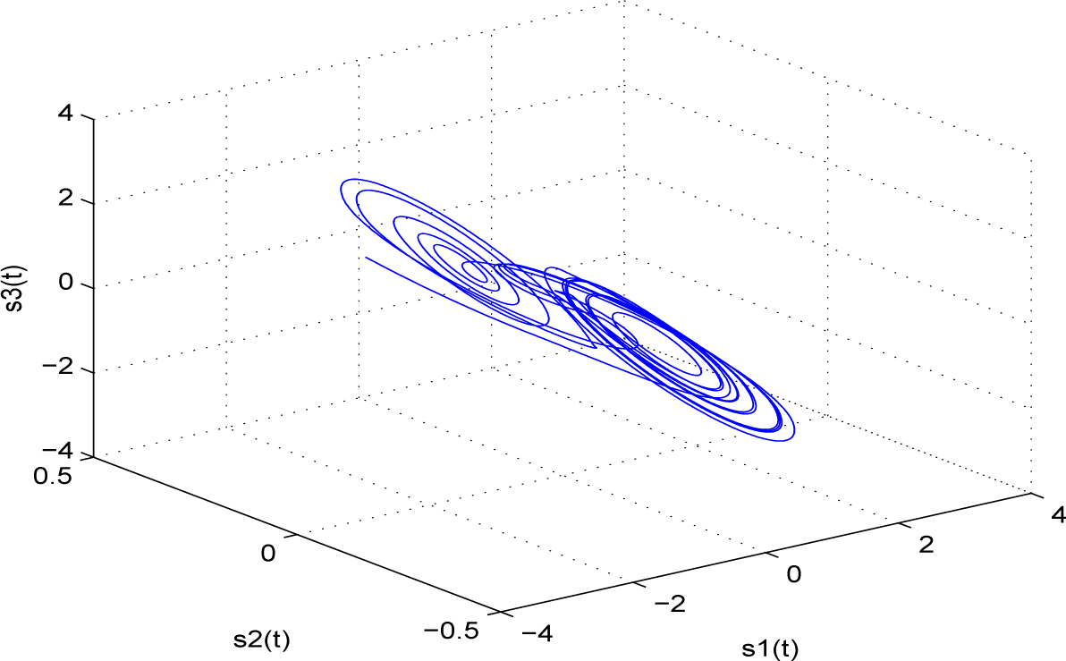
In order to show the effectiveness of the proposed method, we present one numerical example, which is finite-time synchronized for complex networks with N identical nodes, where each node is Chua’s chaotic circuit, and it has a chaotic attractor displayed in Figure 1.
The complex networks consisting of four nodes is described by:
where:
It is noted that the Lipschitz constant [2] of Chua’s circuit is ω = 5, where c0 = 2. Here, the initial conditions of each nodes are chosen:
Coupling matrix G and Γ are given by:
Take σi(x(t)) = diag(xi1 − xi+1,1, xi2 − xi+1,2, xi3 − xi+1,3), x5(t) = x1(t), i = 1,2,3,4. We can verify that Assumption 2 is satisfied. Since:
We can obtain:
Therefore, Assumption 2 is satisfied.
The controllers are chosen as:
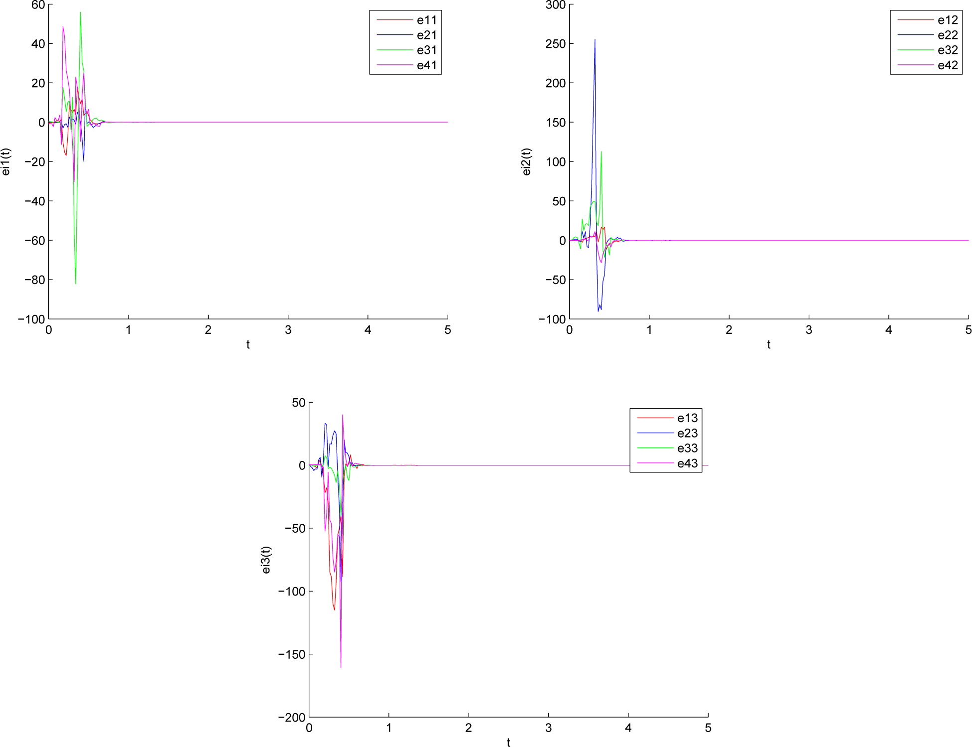
In order to show the original behavior of complex networks (22), the trajectories of the error signals without the controller are depicted in Figure 2.
There exists a positive constant ρ = 1.5, such that:
Therefore, it follows from Theorem 1 that complex networks (22) are finite-time synchronized with the controllers (24). Figure 3 shows the time responses of the error variables ei1(t), ei2(t), ei3(t) for i = 1,2,3,4. It can be seen that the controllers (24) can synchronize complex networks (22) at about t = 0.7s, which is smaller than
. It is obvious that the synchronization time obtained using Theorem 1 is shorter than that obtained by Corollary 1. It is worth pointing out that we were not here concerned with the computational complexity and the computational burden of our approach is similar to that of the method in [24].
5. Conclusions
In this paper, the finite-time synchronization of stochastic complex networks has been studied by finite-time stability theory and inequality techniques. Some sufficient conditions are obtained to ensure finite-time synchronization for the complex networks. The results of this paper are applicable to both directed and undirected weighted networks. In addition, the method in this paper can also be extended to investigate the finite-time synchronization of time-varying networks, such as in [3]. Additionally, under appropriate conditions, a further issue is worth addressing the finite-time consensus of the discrete-time multiagent systems, such as [27,28]. Finally, one example is given to demonstrate the effectiveness of the proposed method.
Acknowledgments
The authors are grateful for the support of the National Natural Science Foundation of China (61174216, 61304162, 61273183, 61374028), the Scientific Innovation Team Project of Hubei Provincial Department of Education (T200809) and the Graduate Scientific Research Foundation of China Three Gorges University (2014PY063).
Author Contributions
Both authors jointly worked on deriving the results and wrote the paper. Both authors have read and approved the final manuscript.
Conflicts of Interest
The authors declare no conflict of interest.
References
- Newman, M.E.J. The structure and function of complex networks. SIAM Rev 2003, 45, 167–256. [Google Scholar]
- Lee, T.H.; Park, J.H.; Ji, D.H.; Lee, S.M. Guaranteed cost synchronization of a complex dynamical network via dynamic feedback control. App. Math. Comput 2012, 218, 6469–6481. [Google Scholar]
- Lü, J.; Chen, G. A time-varying complex dynamical network model and its controlled synchronization criteria. IEEE Trans. Autom. Control 2005, 50, 841–846. [Google Scholar]
- Chen, L.; Qu, J.; Chai, Y.; Wu, R.; Qi, G. Synchronization of a class of fractional-order chaotic neural networks. Entropy 2013, 15, 3265–3276. [Google Scholar]
- Zhao, M.; Zhang, H.; Wang, Z.; Liang, H. Observer-based lag synchronization between two different complex networks. Commun. Nonlinear Sci. Numer. Simul 2014, 19, 2048–2059. [Google Scholar]
- Zheng, S.; Dong, G.; Bi, Q. Impulsive synchronization of complex networks with non-delayed and delayed coupling. Phys. Lett. A 2009, 373, 4255–4259. [Google Scholar]
- Tan, S.; Lü, J. Characterizing the effect of population heterogeneity on evolutionary dynamics on complex networks. Sci. Rep 2014, 4. [Google Scholar] [CrossRef]
- Cao, J.; Lu, J. Adaptive synchronization of neural networks with or without time-varying delay. Chaos 2006, 16. [Google Scholar] [CrossRef]
- Zhang, Q.; Lu, J.; Lü, J.; Tse, C.K. Adaptive feedback synchronization of a general complex dynamical network with delayed nodes. IEEE Trans. Circuits Syst. II 2008, 55, 183–187. [Google Scholar]
- Liang, Y.; Wang, X.; Eustace, J. Adaptive synchronization in complex networks with non-delay and variable delay couplings via pinning control. Neurocomputing 2014, 123, 292–298. [Google Scholar]
- Yu, W.; Chen, G.; Lu, J.; Kurths, J. Synchronization via pinning control on general complex networks. SIAM J. Control Optim 2013, 51, 1395–1416. [Google Scholar]
- Sun, H.; Li, N.; Zhao, D.; Zhang, Q. Synchronization of complex networks with coupling delays via adaptive pinning intermittent control. Int. J. Autom. Comput 2013, 10, 312–318. [Google Scholar]
- Li, C.; Chen, G. Synchronization in general complex dynamical networks with coupling delays. Physica A 2004, 343, 263–278. [Google Scholar]
- Guo, X.; Li, J. Stochastic synchronization for time-varying complex dynamical networks. Chin. Phys. B 2012, 21. [Google Scholar] [CrossRef]
- Yang, X.; Cao, J.; Lu, J. Stochastic synchronization of complex networks with nonidentical nodes via hybrid adaptive and impulsive control. IEEE Trans. Circuits. Syst. I 2012, 59, 371–384. [Google Scholar]
- Karimi, H.R. A sliding mode approach to H∞ synchronization of master-slave time-delay systems with Markovian jumping parameters and nonlinear uncertainties. J. Frankl. Inst 2012, 349, 1480–1496. [Google Scholar]
- Wang, B.; Shi, P.; Karimi, H.R.; Wang, J. H∞ robust controller design for the synchronization of master-slave chaotic systems with disturbance input. Model. Identif. Control 2012, 33, 27–34. [Google Scholar]
- Karimi, H.R.; Gao, H. New delay-dependent exponential H∞ synchronization for uncertain neural networks with mixed time delays. IEEE Trans. Syst. Man Cybern. B 2010, 40, 173–185. [Google Scholar]
- Zhao, Y.; Li, B.; Qin, J.; Gao, H.; Karimi, H.R. Consensus and synchronization of nonlinear systems based on a novel fuzzy model. IEEE Trans. Cybern 2013, 43, 2157–2169. [Google Scholar]
- Luo, R.; Wang, Y. Finite-time stochastic combination synchronization of three different chaotic systems and its application in secure communication. Chaos 2012, 22. [Google Scholar] [CrossRef]
- Wang, H.; Han, Z.; Xie, Q.; Zhang, W. Finite-time chaos synchronization of unified chaotic system with uncertain parameters. Commun. Nonlinear Sci. Numer. Simul 2009, 14, 2239–2247. [Google Scholar]
- Liu, X.; Park, J.H.; Jiang, N.; Cao, J. Nonsmooth finite-time stabilization of neural networks with discontinuous activations. Neural Netw 2014, 52, 25–32. [Google Scholar]
- Sun, Y.; Li, W.; Zhao, D. Finite-time stochastic outer synchronization between two complex dynamical networks with different topologies. Chaos 2012, 22. [Google Scholar] [CrossRef]
- Yang, X.; Cao, J. Finite-time stochastic synchronization of complex networks. Appl. Math. Model 2010, 34, 3631–3641. [Google Scholar]
- Li, B. Finite-time synchronization for complex dynamical networks with hybrid coupling and time-varying delay. Nonlinear Dyn 2014, 76, 1–8. [Google Scholar]
- Chen, W.; Jiao, L. Authors’ reply to “Comments on ‘Finite-time stability theorem of stochastic nonlinear systems”’. Automatica 2011, 47, 1544–1545. [Google Scholar]
- Chen, Y.; Lü, J.; Yu, X.; Lin, Z. Consensus of discrete-time second-order multiagent systems based on infinite products of general stochastic matrices. SIAM J. Control Optim 2013, 51, 3274–3301. [Google Scholar]
- Chen, Y.; Lü, J.; Lin, Z. Consensus of discrete-time multi-agent systems with transmission nonlinearity. Automatica 2013, 49, 1768–1775. [Google Scholar]
Figure 1.
The chaotic behavior of Chua’s circuit with initial condition s(0) = (0.1,0.5,−0.7)T

Figure 2.
Error signals without controllers.

Figure 3.
Error signals with controllers (24).
Figure 3.
Error signals with controllers (24).

© 2015 by the authors; licensee MDPI, Basel, Switzerland This article is an open access article distributed under the terms and conditions of the Creative Commons Attribution license (http://creativecommons.org/licenses/by/4.0/).
Share and Cite
MDPI and ACS Style
Li, L.; Jian, J. Finite-Time Synchronization of Chaotic Complex Networks with Stochastic Disturbance. Entropy 2015, 17, 39-51. https://doi.org/10.3390/e17010039
AMA Style
Li L, Jian J. Finite-Time Synchronization of Chaotic Complex Networks with Stochastic Disturbance. Entropy. 2015; 17(1):39-51. https://doi.org/10.3390/e17010039
Chicago/Turabian StyleLi, Liangliang, and Jigui Jian. 2015. "Finite-Time Synchronization of Chaotic Complex Networks with Stochastic Disturbance" Entropy 17, no. 1: 39-51. https://doi.org/10.3390/e17010039