Non-Extensive Entropy Econometrics: New Statistical Features of Constant Elasticity of Substitution-Related Models

Abstract
: Power-law (PL) formalism is known to provide an appropriate framework for canonical modeling of nonlinear systems. We estimated three stochastically distinct models of constant elasticity of substitution (CES) class functions as non-linear inverse problem and showed that these PL related functions should have a closed form. The first model is related to an aggregator production function, the second to an aggregator utility function (the Armington) and the third to an aggregator technical transformation function. A q-generalization of K–L information divergence criterion function with a priori consistency constraints is proposed. Related inferential statistical indices are computed. The approach leads to robust estimation and to new findings about the true stochastic nature of this class of nonlinear—up until now—analytically intractable functions. Outputs from traditional econometric techniques (Shannon entropy, NLLS, GMM, ML) are also presented.1. Introduction
This paper proposes a new approach for modeling stochastic non-linear inverse problems. The approach is based upon Kullback-Leibler (K–L) relative entropy [1] which then is generalized through a Levy-unstable PL process. The PL structure of below estimated models is first shown. Next, a parameter estimation of three stochastic CES-related models is carried out. A CES is a property of some supply and utility functions which refers to a particular type of aggregator function combining two or more types of supply inputs or demand items into the aggregate quantity.
The first of these three models is the CES production stochastic function. In the case of production system, the fact that this aggregator model exhibits technical CES means that a constant percentage reduction in the quantity of one factor (e.g., labour) must be compassed by one extra unit of another factor (e.g., capital), so that total producer output remains unchanged. The second model is the constant elasticity of commercial substitution model (CECS) which aggregates domestic and imported demand for goods. According to Armington’s contribution related to merchandise demand theory [2], the idea behind the CECS model is that two tradable goods of the same kind will be considered as distinct—and then as plausible perfect substitutes—only on the basis of their geographical origin (region or country). Under a free market assumption, households optimize their utility function by choosing the optimal quantity of each of the two substitutable components. Thus, CECS suggests that a constant percentage reduction in the quantity of one commodity (e.g., locally produced goods) must be compassed by one extra unit of another commodity (e.g., imported goods), so that total household utility remains unchanged. The third is the constant elasticity of technical transformation function (CET) which is aggregating a domestic and export product supply under the above mentioned Armington assumption about differentiated commodities. For profit-maximizing firms, the CET function displays production possibility frontier owing to domestic production allocation to the export market or the domestic market depending on the relative prices of these goods. In Section Seven, additional explanations related to the elasticity of substitution concept will be provided. The importance of these functions is well known by econometricians and other economists, particularly those interested in applied general equilibrium modeling.
Structurally, the CES production model displays causality relationships between supply and input factors. The CECS remains a quasi-identity utility function since it is just missing a quasi-constant variable (the indirect taxes) to constitute an identity. The CET model remains an identity equation, covariate values of which sum up to the explained value of the model, suggesting that national production aggregates two classes of goods (the locally demanded product and the export product). These two goods are supplied through a constant elasticity of technical transformation [3].
Thanks to the proposed non-extensive entropy approach—enabled by PL characterization of CES functions—implications on the stochastic features of these three distinct models are pointed out through robust estimation procedure. To our knowledge, this nonlinear class of functions remains analytically intractable when using traditional statistical techniques. This constitutes the main contribution of the paper.
The document is organized as follows: Section 2 presents some transitional properties linking PL and low frequency time series. Section 3 eclectically presents the PL nature of the CES function. Section 4 generalizes the Kullback-Leibleir divergence entropy to non-ergodic systems and discusses constraining problems of such models in the context of the generalized non-extensive entropy econometric model presented in Section 5. Section 6 presents some formalisms related to the parameter confidence area of the model. Finally, Section 7 presents the outputs of the model and Section 8 gives concluding remarks.
2. Tsallis Non-Extensive Entropy and Low Frequency Series Modeling
Parameters of the proposed nonlinear models were estimated on the basis of an annual time scale statistical sample. We consider that PL-related Tsallis entropy will still exist, even in the case of low frequency series, a valuable device for aggregated data modeling since the outputs provided by exponential family law, e.g., the Gibbs-Shannon entropy approach, correspond to the limiting case of Tsallis entropy when the Tsallis q-parameter equals unity. Next, perhaps more a pertinent argument for using Tsallis non-extensive entropy formalism is the existence of a number of complex phenomena involving long-range correlations, still observable when data is time scale-aggregated [4,5]. This could be due to interaction between the functional relationships describing the involved phenomena and the inheritance properties of PL or could depend on their non-linearity.
Delimiting the threshold values of the PL path towards the Gaussian distribution (or to the exponential family law) as a function of the data frequency level remains statistically difficult since each phenomenon may display its own speed of convergence—if any—towards the central limit theorem attractor. The next source of statistical concern may be related to systematic errors from statistical data collecting and processing which can generate a kind of heavy distribution. Thus, a systematic application of the Shannon-Gibbs entropy approach in the above cases—even on the basis of annual data—could be misleading and, in the best case, lead to instable solutions. Having in mind that non-extensive Tsallis entropy generalizes the exponential family law [6,7], the q-Tsallis entropy approach fits high or low frequency series. Next, as pointed out in [8,9], among a few types of higher-order entropy estimators, able to generalize the Gaussian law, Tsallis non-extensive entropy displays the property of concavity, —thus stability—along the existence interval which characterizes most real world phenomena. Furthermore, the q-generalization of the K–L information divergence [10,11] parameter conserves the same basic properties as the standard K–L cross-entropy and remains usable for a similar purpose [9]. As a final point, the q-Tsallis index displays an expected quality of assessing complexity degree of random systems with respect to the Gaussian benchmark. Some of the positive returns may concern the monitoring of the quality of collected statistical data or the potential distribution law.
3. PL and the CES Function
In the early 1960s, Arrow, Chenery, Minhas, and Solow [12,13] set up a new nonlinear function simultaneously displaying the property of homogeneity, CES between factors of production, and differentiating elasticity of substitution for various industries, sectors, or countries [14]. In empirical research, due to the impossibility of successfully estimating parameters of that function, calibration technique has so far been used. Less adequate outputs owing to such empirical approach have led a large community of economists to question the rationale of some economic modeling techniques like the applied general equilibrium approach. In this Section, we develop the proposed entropy formalism using a classical CES production model (CESP) explaining the gross domestic product (VAt) by two classical factors (e.g., [14,15]): Labor (Lt) and capital (Kt). The next two CES model class cases will be presented in Section 7. Below we present the mathematical form of a CES production model:
or one of its generalized formulations as:
where:
and τe is a CES between factors; εt stands for the random disturbance with unknown distribution. In Equation (1), α stands for the shift parameter; the parameter δ belongs to the interval between zero and one and represents the share (distribution) of the sold quantities of both distributed factors. Parameter ν reflects the degree of changing returns of VAt to scale. The higher the value of r, the higher the degree of substitution between factors. The case of τe converging to 0 suggests perfectly substitutable factors. In the case of more than two inputs Xi, ( ), we get the generalized form in Equation (2).
Let us now focus on the connection between the CES class of functions and a PL. In fact, to better display that relation, let us aggregate components of Model (1) into one variable without conserving additivity. Then, we get a generic case of a PL of the form:
where in this case the endogenous variable VAt is the product per head. Parameter β represents a general level of technology. The variable kt stands for a capital coefficient. The exponent h belongs within the interval (−1, +∞) and defines a per head product elasticity with respect to the capital coefficient. The random term εt, itself, is assumed to follow PL structure. Index t means time period. Thus, such characterized PL relationships between the class of the CES functions seems to bear potential implications on economic grounds, including extensions to the financial side of economy. A PL displays interesting properties that may explain its ubiquity at different complexity levels, in natural or manmade systems. For a survey on the inheritance mechanism and other properties of PL, see, for instance, Gabaix [16]. For the direct relationships between a PL and non-extensive Tsallis entropy, see, for instance, Tsallis C. [9]. The proposed model generalizes the statistical theory of information approach to non-ergodic systems, that is, those in which probabilities pi of microstates to “visit” the system are not identical [8]. There are many other forms of generalized entropy. However, only Tsallis entropy assures concavity (stability) over an interval where the q-Tsallis parameter is higher than unity. Since many physically meaningful phenomena for which q is higher than unity dominate in the physical world, this becomes a serious drawback of rival entropies. In the next section, we present a connection between the classical Gibbs-K–L cross-entropy formalism and the more general Tsallis relative entropy.
4. q-Generalization of the K–L Information Divergence and Constraining Problems
The K–L index of information divergence [1] is q-generalized in a straightforward way, as follows [9]:
or in discrete case:
stands for the traditional K–L index of information divergence between hypotheses p and p(0), under the hypothesis that q is equal to unity. It is worth emphasizing that the above generalization does not alter estimator properties of K–L information index presented e.g., in [1]. There are two main versions of K–L divergence in Tsallis statistics. The first is the traditional generalized K–L shown above and the second is the generalized Bregman K–L. As presented by [11], there are still difficulties in empirical applications while trying to reconcile the above versions of the models. In the same study, authors reveal interesting aspects when q-generalized cross-entropy is associated with constraining information. Authors [15] suggest the q-generalized cross-entropy, defined later by Equation (11), to be more consistent with the expectations and the constraints form proposed by [17] known as q-averages or escort distribution:
However, as is shown in our recent article (in press), the Curado-Tsallis [18] constraints of the form:
seem to lead to more stable outputs. In the present work, in reverse, Escort distribution (12) seems more appropriate.
5. A Generalized Non-Extensive Entropy Econometric Model
Both in the pioneering work on maximum entropy econometrics by authors [19] and in the work of author[15], the moment-constraints of an entropy econometric linear model for ergodic systems have been reparameterized [20]. We need to transform variables of the constraining generalized linear model into weight-probabilities over a point support space defining each of the original random parameters. Let us now consider the next general linear model Y of the form:
where unknown B parameter values are not necessarily constrained between 0 and 1, which suggests the necessity of reparametrization. The term ε is an unobservable disturbance term, plausibly with finite variance—owing to the nature of economic data—exhibiting observation errors from empirical measurement or from random shocks. These stochastic errors are assumed to be driven by PL, as suggested in the introductory section of this document. The variable Y represents a system and X accounts for covariates generating the system through relation parameter matrix B and unobservable disturbance ε to be estimated through observable error components e. Next, treating each Bk(k=1…K) as a discrete random variable defined over a compact support space[15,19] and 2 < M < ∞ possible outcomes, it is then possible to express Bk as:
where pkm are non-negative outcome probabilities vkm which must sum up to unity. Likewise, if we treat each component ei of e as a finite and discrete random variable defined over a compact support space and possible outcomes centered around zero, we formulate ei as follows:
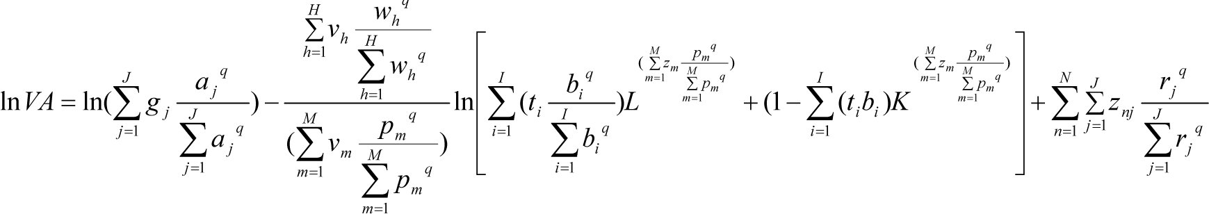
where rn is the outcome probability of zn on the support space j. As usually adopted, the index n will designate the number of statistical observations. The error component e can be set up as a fraction of the endogenous variable, as an a priori Bayesian hypothesis. Since we do not constrain the model to conjugated distributions, posterior probability outcome within the support space may display a non-Gaussian structure. The element vkm constitutes a priori information while pkm is an unknown posterior whose value results from the solving process of the information divergence problem. Let us rewrite B = V · P with and in matrix notation, where, again, K stands for the number of parameters to be estimated and M the number of data points on the support space. Likewise, let , with and for N be the number of observations and J the number of data points on the support space for the error component. Finally, applying an escort distribution in moments, the Tsallis cross-entropy econometric model is stated as:
Subject to:

For reasons of formal presentation, the criterion function Equation (11) has excluded probabilities wh, explaining the degree of economy changing to scale and bi, the distribution parameter between factors. As we know, additional a priori information added to Equations (11)–(15) will improve the quality of the estimated parameter. In the present case, since CES model formulation is based on economic theory, we could for instance predict its sign value domain variation for each parameter. Then, we get:
where α, ρ, δ from Equation (1) stands for the original, “before-reparameterization” parameters. The set G,Z,T stands for the above original parameter support space with the corresponding weight-probabilities a, p, b defining output posteriors. We include all the support spaces G,Z,T in the general support space v, Equation (9), aggregating all the parameters of the constraining equation system. Here we just present how we have specified the present model and not a general rule of specification. Note that depending on error distribution, the weights α, β introduced in the above dual objective function, may exercise a significant impact on the model optimal outputs through the Lagrange multipliers which link the constraining information with the criterion function.
6. Parameter Confidence Area
In this section, we follow the reference work of [19] or that of [15] and set up an inference information index s(aj) as an equivalent to a standard parameter error measure in the case of classical econometrics. A coefficient comparable to determination coefficient R2 is proposed under the entropy symbol S(Pr). We first recall that the maximum level of entropy-uncertainty is reached provided that the non-relevant information-moment constraints are enforced. Such a maximum corresponds to a uniform probability distribution over the k states of the system. Next, each new piece of informative data in the form of a restrictions leads to a departure from the uniform distribution, meaning an uncertainty shrinkage. Accordingly, the normalized level of the S(Pr) will reflect, for the whole model, a departure from the maximum uncertainty. Taking into account the above and following the formulations in [19] let us propose a normalized non-extensive entropy measure of s(aj) and S(Pr). Let us refer to Tsallis entropy property, Sq > 0, and consider all possible micro-states of the system. This number varies with the number of the support space data points i (i = 1..M) and the number of parameters of the model j (j = 1..j). Entropy Sq vanishes (for all q) in the case of ; for , q > 0, whenever one of the pi (i = 1..M) occurrences equals unity, the remaining probabilities will vanish. We get a global, absolute maximum of Sq (for all q) in the case of a uniform distribution, i.e., when all . When such an instance distribution occurs, the maximum entropy is explained as follows:
and:
In Equation (20) n varies with the number of model observations and the number of the support space data points generating the parameter. Below [15] is a normalized entropy index with the numerator representing the calculated entropy of the system and the denominator displaying the highest maximum entropy Equations (19) and (20):
with j varying from 1 to j (the quantity of parameters in the model) and i belonging to M (the quantity of support space points), with M > 2. Multiplying the number of model parameters J by the number of support space points M with M > 2, we get the total number of micro-states. Thus s(aj) conveys information on the precision of the estimated parameters. The next Equation, (22), reflects the non-additivity Tsallis entropy property for any two independent systems. As we are dealing with stochastic systems, the first term S(p) is related to the probability distribution of the parameter and the second S(r) to the disturbance probability of the error:
where:
and:
explains the sum of the normalized entropies related to the model parameters , and to the disturbance term . Similarly, the above value is derived for all observations n, with F, the number of data points on the support space of the estimated probabilities r, related to the error term. We note that the values of entropy indexes , are normalized. Index value near unity is an indication of a poor informative variable—with higher entropy—while lower index values indicate a better informative variable about the stochastic system.
As far as estimator properties are concerned, both indexes fulfill the basic Fisher-Rao-Cramer information index properties, including continuity, symmetry, maximum, and additivity [1]. In fact, as suggested in [9], the q-generalization of K–L information divergence Equations (5) and (6) keeps unchanged the basic estimator properties of K–L information divergence model.
7. Model Outputs and Discussion
This section presents outputs of the three computed constant elasticity class models. The first was presented in detail in Section 3 as a CES production function Equation (1). The next two models are the CECS known as the Armington model Equation (23) and the CET Equation (24), already alluded to in the introduction Section. As already mentioned, the estimation outputs presented in this Section allow for validating the three above model stochastic features thanks to non-extensive Tsallis entropy formalism. We compare the outputs from the non-extensive cross-entropy (NCE) with those from the traditional estimation techniques: The non-linear least squares (NLLS), the generalized methods of moments (GMM), and the maximum likelihood approaches (e.g., [21,22]). Statistical data used for model estimation come from Eurostat web site and are presented in the Table 1.
Before undergoing the computation procedure, data have been dimensioned at logarithmic scale. The computations of the NCE model were carried out with the General Algebraic Modeling System (GAMS) code. Those with the NLLS technique were done in a common spread sheet (Microsoft Excel). Computations by the GMM and ML approaches were executed with special code from the open source GRETL.
Let us first show mathematical formulation of the next two CES model classes. A CECS utility function of domestic economic absorption aggregator (Ct) of two business components (locally produced commodities demand (DO) and imports demand (M) has the following analytical form:
where
with τe CES, δ and εt standing, respectively, for distribution parameter and random disturbances with unknown distribution.
The last model CET, the technical transformation function aggregator (MOt), is analytically formulated in the following way:
where:
and EXt, DMOt stand, respectively, for exports, and domestically marketed outputs. The rest of the symbols have the same meaning as in the previous models. The higher the value of ρ, the higher the degree of transformation. When that parameter converges to −∞ we are dealing with the case of perfectly complementary products, which refers to Leontief technology. The case of r converging to −1 suggests perfectly substitutable products.
For a clearer understanding of model outputs, let us first recall a key concept of elasticity of substitution (ES). It represents the percentage change in the ratio of consumption of two different commodities (or two factors of production) due to the variation of the marginal rate of substitution (MRS) between the two commodities (or two factors of production). Next, MRS is the rate at which a consumer (producer) is ready to give up one commodity (factor of production) in exchange for another commodity (factor of production) while maintaining the same level of utility (production). Formally, assuming free market conditions, if we let the utility over consumption of two commodities (c1 and c2) be explained by , ES is defined as follows:
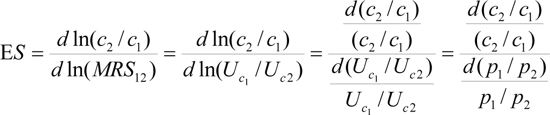
The last equality which explains is just presented to render clearer the empirical side of ES. It is a relationship from the first order condition for a consumer utility maximization problem. Intuitively, it shows how a consumer's relative choices over consumption items change as their relative prices change.
In this study, priors were initiated from NLLS outputs. As known, such priors are not deterministically fixed. They are updated according to the Bayesian information processing rule. For simulation purposes, different q-Tsallis parameter values were computed from unity to its admissible highest values minimizing the criterion function over an interval covering Gaussian ( ) and stable laws (e.g., Levy’s attractors for ). In all models, an a priori parameter support space for reparameterization varies between −5.0 and +5.0. The same prior space has been retained for the error disturbance, with amplitude varying between −3 and +3, so it conforms to the three sigma rule owing to the Chebyshev’s inequality [23]. Both spaces are symmetric around zero. This prevents the estimated parameters from a bias.
Tables 2–5 comparatively display the outputs from, respectively, the NCE, NLLS, GMM, and ML techniques for each of the three models. The NCE estimator super-consistency for all three models can be noticed in spite of the very small sample used.
As suggested in the Introduction, each of the above three models displays its particular stochastic level. Only the new presented Tsallis NCE estimator replicates these differences. This is so because, as already shown in Equation (4), the CES-related model displays a data generating PL system. The NLLS approach seems to be better than the GMM procedure. The ML produces, as theoretically expected, much poorer outputs.
Using traditional nonlinear, least square methods, we have linearized the Equations (1), (23) and (24) before applying the Taylor development and the LS approaches [21].
In the case of the CESP and CECS models, the GMM computation procedure has been initialized with: A = 0.700, δ = 0.71, ρ = 0.28, and ν = 0.61 for exclusively the CESP model. In the case of the CET model, those values were A = 0.700, δ = 0.497, ρ = 0.5025.
The next technique applied is the ML. In the case of the production model CESP, we have initialized the model with: A = 2.2500, δ = 0.5, ρ = 0.9, ν = 1; in the CET model, we used A = 1.750, δ = 0.6, ρ = −990; and finally in the CECS model estimation, we started with: A = 1.750, δ = 0.6, ρ = −950.
Coming back to the NCE outputs, the estimated parameters reflect long-run optimal equilibrium values of the system. Taking into account the fact we are dealing with the aggregated accounts of 27 EU countries, the estimated parameters remain consistent with our expectations. For instance, in the case of the CESP production model, the estimated parameter p with an estimate close to zero suggests a convergence of the analysed CES model to the classical Cobb-Douglas model, displaying constant returns to scale. A long-run, optimal equilibrium share parameter ∂ between factors shows a lower proportion of labor of around 16% with respect to physical capital share (84%). In 2010, this proportion was around 57% for labor. For the CET and CECS models, the estimated parameters show, in the long run, a quasi-perfect substitutability and a balanced share between local and foreign commodities. All the above models present an error coefficient variation (CV) around zero. By definition, the CV index is obtained by dividing the model standard error by the average value of dependent variable. The Tsallis Information index presented in the previous paragraph is around unity for the three models, suggesting relatively close to zero information divergence between priors and posteriors, under given model restrictions. We would have expected optimal solutions for q less than 5/3 or, in the worst case, less than 2, for theoretical and empirical evidence. This is the case for the two commercial models, CET and CECS, where q is almost equal to unity, suggesting a Gaussian distribution.
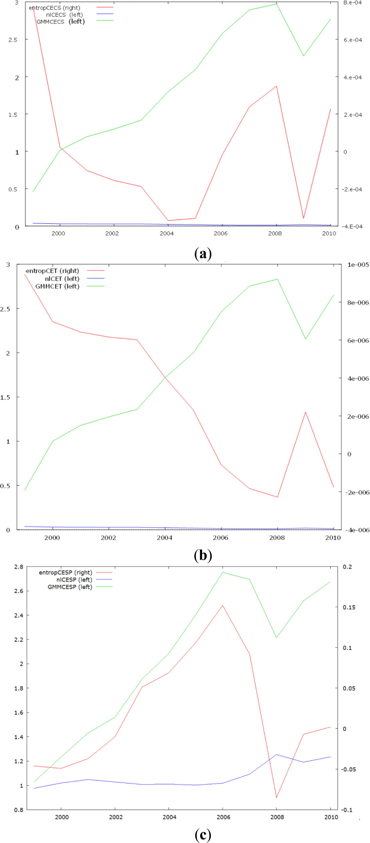
The model quality is likewise shown in Figures 1(a–c), which display the component errors generated by each estimation approach. We note from these figures that only the error distribution from the Tsallis entropy approach (red line), over a 12-year period, seems to alternate the signs around zero (see right side of figure rectangles). This is true for each of the three models. Estimators from the remaining competitive techniques remain biased for this class of models. Next, the highest performance of the CET model is naturally due to its identity nature.
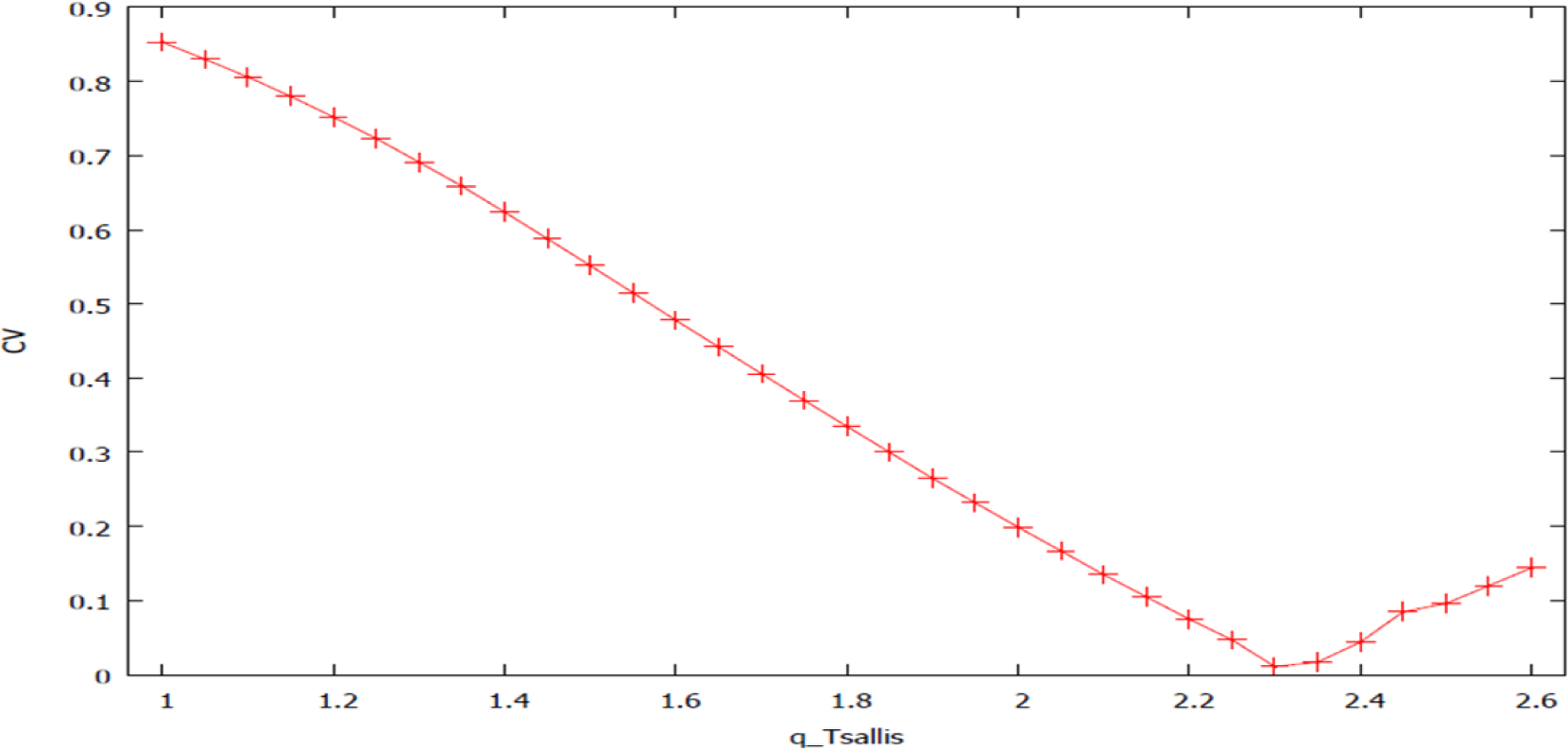
For the CESP production model, minimum LS errors are obtained for q around 7/3 (Figure 2). This value of q ∈ (5/3, 3) characterizes Lévy distribution, noting that we have 3 degrees of freedom (3 independent parameters) in the considered nonlinear Equation (1) defining—over a twelve-year period—the complexity of the system. Surprisingly enough, comparable outputs from different research areas do exist. In a recent study using Tsallis cross-entropy formalism to optimize noise-aided information transmission via stochastic resonance [24], authors found the optimal Tsallis q-parameter around 2.3. Other authors [25] found q ∈ (2,2.3) in a recent study on “the size distributions of non-coding DNA (including introns and intergenic regions) in all human chromosomes.” To my knowledge, any scientific explanation of such converging Tsallis q-parameter values around 7/3 has not yet been presented. Moreover, Tsallis q-parameter with higher values have been found in some recent economic studies. For instance, author [26] found “cumulative distribution of the scaled gross domestic product of 167 countries around the world for the year 2000 corresponding to q = 3.5”. The q-parameter has been incremented by a step of 0.25 starting from unity (Shannon entropy point). Figure 2 displays a convex space defining different optimal CV values owing to different simulated q-Tsallis parameters for the CESP model. Minimum CV corresponds to the minimum of information divergence or of the sum of geometrical error of least squares.
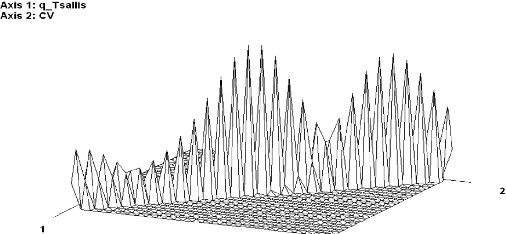
To verify the Tsallis related model outputs, we have computed a classical S-K-L cross-entropy econometric model, which, as expected, has produced the same values as those obtained from Tsallis formalism for q equal to unity for all three models. Such relatively trivial results have not been reported in the above output tables. In the case of the CESP model, we found for q converging to unity a CV of 85.3% in the case of K–L, against 0.06% for an optimal q equal to 2.331. Thus, this point shows the advantage of modeling with non-extensive entropy rather than the Shannon method, reduced to q equal unity. The last figure (Figure 3) is an attempt to depict relationships between the different optimal CV displayed in Figure 2.
We seem to observe a kind of invariant scale error structure at three levels, along with the q-parameter steadily evolving on a convex space towards the global minimum point of the model where q equals 2.331. The non-reported in the document observations on the autoregressive error process of the CESP model indicate a plausible presence of a fractionally integrated moving average (ARFIMA) error structure. All the noticed degrees of error lag seem to alternate—over a short-period experiment—positive and negative autocorrelation, suggesting an “over-differencing.” This point should remain in compliance with the PL nature of a CES function.
8. Concluding Remarks
The present work has developed a new Tsallis cross-entropy econometric approach for instable, nonlinear econometric models. A large class of economic and financial models should fall into this category. We have limited our study to the three CE class functions with three distinctive stochastic forms. Only outputs produced by Tsallis formalism reflect these stochastic differences. A Super-convergence of the Tsallis entropy estimator should be owing to a strong similarity between the sample and the data generating PL system. Furthermore, we have noted a plausible presence of a fractionally integrated moving average (ARFIMA) error structure. More investigation is needed to confirm the proposed PL-based approach for econometric modeling.
Acknowledgments
The author gratefully acknowledges University of Information Technology and Management in Rzeszow (Poland) for having financed this research.
Conflicts of Interest
The authors declare no conflict of interest.
PACS Codes: 89.65.Gh; 89.70.cf
References
- Kullback, S.; Leibler, R.A. On information and sufficiency. Ann. Math. Stat 1951, 22, 79–86. [Google Scholar]
- Armington, P.S. A. Theory of demand for products distinguished by place of production. Int. Monet. Fund Staff Pap 1969, 16, 159–178. [Google Scholar]
- Gruen, F.H.G.; Powell, A.A. The Constant elasticity of transformation production frontier and linear supply system. Int. Econ. Rev 1968, 9, 315–328. [Google Scholar]
- Kwapień, J.; Drożdż, S. Physical approach to complex systems. Physica Rep 2012, 515, 115–226. [Google Scholar]
- Rak, R.; Kwapień, J.; Drożdż, S. Nonextensive statistical features of the Polish stock market fluctuations. Physica A 2007, 374, 315–324. [Google Scholar]
- Dragulescu, A.; Yakovenko, V.M. Exponential and power-law probability distributions of wealth and income in the UK and the USA. Physica A 2001, 299, 213–221. [Google Scholar]
- Nielsen, F.; Nock, R. A closed-form expression for the Sharma-Mittal entropy of exponential families. J. Phys. A 2012, 45, 032003. [Google Scholar]
- Gell-Mann, M.; Tsallis, C. Nonextensive Entropy, Interdisciplinary Applications; Oxford University Press: New York, NY, USA, 2004. [Google Scholar]
- Tsallis, C. Introduction to Nonextensive Statistical Mechanics: Approaching a Complex World; Springer: Berlin, Germany, 2009. [Google Scholar]
- Bağci, G.B.; Arda, A.; Sever, R. On the problem of constraints in nonextensive formalism: A quantum mechanical treatment. Int. J. Mod. Phys. B 2006, 20, 2085–2092. [Google Scholar]
- Plastino, A.R.; Venkatesan, R.C. Deformed Statistics K-L Divergence Minimization within a Scaled Bregman Framework. Phys. Lett. A 2011, 375, 4237–4243. [Google Scholar]
- Arrow, K.J.; Chenery, H.B.; Minhas, B.S.; Solow, R.M. Capital-labor substitution and economic efficiency. Rev. Econo. Stat 1961, 43, 225–250. [Google Scholar]
- Solow, R.M. A contribution to the theory of economic growth. Q. J. Econ 1956, 70, 65–94. [Google Scholar]
- Klump, R.; Papageorgiou, C. The CES Production Function in the Theory and Empirics of Economic Growth. J. Macroecon 2008, 30, 599–600. [Google Scholar]
- Bwanakare, S. Solving a generalized constant elasticity of substitution function of production: A non ergodic maximum entropy principle. Acta Phys. Pol 2013. [Google Scholar] [CrossRef]
- Gabaix, X. PLs in Economics and Finance, Available online: http://www.nber.org/papers/w14299 (accessed on 11 May 2014).
- Mendes, R.S.; Plastino, A.R.; Tsallis, C. The role of constraints within generalized nonextensive statistics. Physica A 1998, 261, 534–554. [Google Scholar]
- Curado, E.M.F.; Tsallis, C. Generalized statistical mechanics: Connection with thermodynamics. J. Phys. Math. Gen 1991. [Google Scholar] [CrossRef]
- Golan, A.; Judge, G.; Miller, D. Maximum Entropy Econometrics: Robust Estimation with Limited Data; John Wiley & Sons: New York, NY, USA, 1996. [Google Scholar]
- Golan, A.; Perloff, J.M. Comparison of Maximum Entropy and Higher-Order Entropy Estimators; University of California: Berkeley, CA, USA, 2001. [Google Scholar]
- Green, W.H. Econometrics Analysis, 5th ed; Prentice Hall: New York, NY, USA, 2003. [Google Scholar]
- Grandy, W.T., Schick, L.H., Eds.; Maximum Entropy and Bayesian Methods; Springer: Berlin, Germany, 1990; pp. 17–31.
- Pukelsheim, F. The Three Sigma Rule. Am. Stat. Assoc 1994, 48, 88–91. [Google Scholar]
- Chapeau-Blondeau, F.; Delahaies, A.; Rousseau, D. Tsallis entropy measure of noise-aided information transmission in a binary channel. Phys. Lett. A 2011, 375, 2211–2219. [Google Scholar]
- Oikonomou, Th.; Provata, A.; Tirnakli, U. Nonextensive statistical approach to non-coding human DNA. Physica A 2008, 387, 2653–2659. [Google Scholar]
- Borges, E.P. Empirical nonextensive laws for the county distribution of total personal income and gross domestic product. Physica A 2004, 334, 255. [Google Scholar]


| Year | 1999 | 2000 | 2001 | 2002 | 2003 | 2004 | 2005 | 2006 | 2007 | 2008 | 2009 | 2010 |
|---|---|---|---|---|---|---|---|---|---|---|---|---|
| VA | 7.82 | 8.136 | 8.427 | 8.578 | 8.978 | 9.294 | 9.76 | 10.288 | 10.288 | 9.777 | 10.149 | 10.412 |
| K | 3.287 | 3.42 | 3.55 | 3.641 | 3.86 | 4.02 | 4.265 | 4.528 | 4.476 | 4.105 | 4.336 | 4.444 |
| L | 4.427 | 4.606 | 4.76 | 4.819 | 4.99 | 5.149 | 5.374 | 5.63 | 5.683 | 5.554 | 5.691 | 5.834 |
| MO | 8.691 | 9.026 | 9.212 | 9.325 | 9.442 | 9.689 | 9.877 | 10.211 | 10.550 | 10.621 | 10.162 | 10.359 |
| DMO | 5.719 | 5.693 | 5.751 | 5.792 | 5.846 | 5.813 | 5.773 | 5.711 | 5.795 | 5.797 | 5.924 | 5.693 |
| Export | 2.971 | 3.333 | 3.461 | 3.533 | 3.596 | 3.876 | 4.104 | 4.500 | 4.754 | 4.825 | 4.238 | 4.666 |
| Imports | 2.938 | 3.272 | 3.361 | 3.414 | 3.526 | 3.796 | 4.029 | 4.411 | 4.672 | 4.727 | 4.153 | 4.551 |
| Exogenousvar: | A | δ | p | v | I(Pr) | CV |
|---|---|---|---|---|---|---|
| CESP(L(t), K(t)) | 1.866 | 0.163 | 0.001 | 1.e+00 | 0.99 | 0.006 |
| CET(DO(t),Ex(t)) | 2.000 | 0.5 | −1.E00 | 0.999 | 4.271E–7 | |
| CECS(C(t),M(t)) | 2.021 | 0.504 | −1.E00 | 0.999 | 2.705E–5 |
q Tsallis parameter (weight αi = 0.05) = 2.333 (CECP); q Tsallis parameter(weight αi = 0.05) = 1.E+00 (CECS); q Tsallis parameter (weight αi = 0.05) = 1.E+00 (CET).
| Exogenous var | A | δ | ρ | ν | R2 |
|---|---|---|---|---|---|
| CESP(L(t), K(t)) | 1.995 | 0.282 | 3.046 | 0.993 | |
| Parameters T-value | 48.89 | 6.61 | 1.49 | 6.61 | 0.88 |
| CET(DO(t),Ex(t)) | 2.008 | 0.497 | −0.954 | ||
| Parameters T-value | 558.12 | 1551.4 | −292.5 | 0.999 | |
| CECS(C(t),M(t)) | 2.147 | 0.477 | −0.532 | ||
| Parameters T-value | 6.257 | 13.073 | −1.554 | 0.83 |
| CESP | CET | CECS | ||||
|---|---|---|---|---|---|---|
| Estimate | Std. Error | Estimate | Std. Error | Estimate | Std. Error | |
| A | 1.672 | 0.007 | 1.647 | 0.003 | 1.679 | 0.024 |
| δ | 0.54 | 0.079 | 0.511 | 0.001 | 0.524 | 0.022 |
| ρ | −1.53 | 1.922 | −2.344 | 0.026 | −1.852 | 0.279 |
| ν | 0.679 | 0.004 | ||||
| CESP | CET | CECS | ||||
|---|---|---|---|---|---|---|
| Estimate | Std. Error | Estimate | Std. Error | Estimate | Std. Error | |
| A | 2.97 | 9.66 | 0.933 | 0.002 | 0.945 | 0 |
| δ | 0.813 | 10.569 | 0.241 | 0.008 | 0.303 | 0.002 |
| ρ | 1.018 | 34.114 | −0.349 | 0.003 | −0.293 | 0.001 |
| ν | 1.145 | 16.903 | ||||
| Akaikecriterion | −26.46 | −267347.1 | −77504.51 | |||
© 2014 by the authors; licensee MDPI, Basel, Switzerland This article is an open access article distributed under the terms and conditions of the Creative Commons Attribution license (http://creativecommons.org/licenses/by/3.0/).
Share and Cite
Bwanakare, S. Non-Extensive Entropy Econometrics: New Statistical Features of Constant Elasticity of Substitution-Related Models. Entropy 2014, 16, 2713-2728. https://doi.org/10.3390/e16052713
Bwanakare S. Non-Extensive Entropy Econometrics: New Statistical Features of Constant Elasticity of Substitution-Related Models. Entropy. 2014; 16(5):2713-2728. https://doi.org/10.3390/e16052713
Chicago/Turabian StyleBwanakare, Second. 2014. "Non-Extensive Entropy Econometrics: New Statistical Features of Constant Elasticity of Substitution-Related Models" Entropy 16, no. 5: 2713-2728. https://doi.org/10.3390/e16052713
APA StyleBwanakare, S. (2014). Non-Extensive Entropy Econometrics: New Statistical Features of Constant Elasticity of Substitution-Related Models. Entropy, 16(5), 2713-2728. https://doi.org/10.3390/e16052713