1. Introduction
Data Envelopment Analysis (DEA) was first introduced by Charnes
et al. [
1] in 1978. DEA has been proved to be an effective methodology for the efficiency evaluation of Decision Making Units (DMUs) with multiple inputs and multiple outputs. In the DEA methodology, the efficiency of a DMU is defined as a ratio of its weighted sum of outputs to its weighted sum of inputs [
2]. A DMU is evaluated as efficient if it has an efficiency score of one. In the traditional DEA models, a DMU is allowed to use its most favorable multiplier weights to achieve its maximum efficiency score. It would however be somewhat irrational that different DMUs are evaluated with different sets of multiplier weights. As a result, there are usually more than one DMU being evaluated as efficient and for these efficient DMUs, traditional DEA models cannot provide further discrimination. Different methods have been developed for this problem, such as the super efficiency model, cross-efficiency model and so on [
2]. However, these mentioned models are still based on different sets of multiplier weights which could be irrational sometimes.
The common weights DEA model is an effective method for solving the problems mentioned above [
2,
3]. The main idea of the common weights DEA method is evaluating different DMUs based on a common set of multiplier weights and this common set of weights is calculated from the DEA models. A most representative model was proposed by Kao and Hung [
4] which aims to minimize the distance between DMUs and the ideal solution. Some extension of the research in [
4] can be found in [
5,
6]. Liu and Peng [
7] also proposed a common weights DEA model based on the idea of minimizing the distance. However the distance in their research is named the virtual gap, which is calculated by a linear program model. Another method of determining common weights is by introducing the ideal and anti-ideal DMU into the DEA model [
8–
11]. Ramon
et al. [
12,
13] extended their research on the cross-efficiency evaluation into the common weights DEA method based on the idea of reducing differences between profiles of weights. Some other techniques have also been introduced into the DEA method for determining common weights, such as goral programming [
14], regression analysis [
15], robust optimization [
16] and so on [
17–
20]. Applications of the common weights DEA models can be found in economy evaluation [
21], technology selection [
22], resource allocation [
23], and so on.
Shannon’s entropy [
24] is a key concept in information theory. Some literatures have combined the DEA method with Shannon’s entropy. As far as we can say, the first such research was proposed by Soleimani-Damaneh and Zarepisheh [
24] in which Shannon’s entropy was used to aggregate efficiency scores from different DEA models. Based on this first research, Bian and Yang [
25] proposed an extension to the resource and environment efficiency analysis of the provinces in China. More recently, Xie
et al. [
26] proposed an extension research of [
24] in which different variable subsets were considered. Similarly, Wu
et al. [
27] proposed a method for aggregating cross-efficiency with Shannon’s entropy and they also extended their research in [
28]. Besides, Yang
et al. [
29] proposed a statistical approach to detect the influential observations in DEA in which the entropy was used to detect the change in the distribution after the DMU is removed. There are also some other researches and applications of entropy in the DEA method [
30–
32], but as far as we know, there has been no research that combines Shannon’s entropy with the common weights DEA.
In this paper, we introduce Shannon’s entropy into the common weights DEA method for improving the discrimination power of DEA. We propose a 6-step computing procedure for calculating the common weights in which Shannon’s entropy is used to determine the importance degree of different DMUs’ optimal weights. Within this computing procedure, we also propose a new model for calculating non-zero optimal weights for each DMU. Some theoretical results are provided and by application to some numerical examples, our proposed method has been proved to be more powerful in discriminating DMUs, especially when the inputs and outputs are numerous. Our proposed model is also accordant with the original DEA methodology considering the evaluation of the best and worst DMUs.
The rest of this paper is organized as follows: in Section 2, some preliminaries are introduced as the background; in Section 3, our proposed methodology with Shannon’s entropy is formulated in detail; in Section 4, some numerical examples are provided as the illustration and examination of our model; finally in Section 5, we give the conclusions.
3. Proposed Methodology with Shannon’s Entropy
In order to improve the discriminating power of the DEA method, we propose a methodology using Shannon’s entropy to aggregate different sets of optimal weights into a common set of weights. Then DMUs could be evaluated with this common set of weights. In our proposed method, we also propose a modified weight restriction model for calculating non-zero weights in DEA. Our proposed methodology can be formulated as the following six steps.
3.1. The Computing Procedure
Step 1: Data normalization. In this paper, we suppose that there is no outlier data in inputs and outputs. For convenience of comparison, the input
and output
of
are normalized as follows:
Remark 1. It should be noted that the inputs and outputs in the DEA problem naturally have different metrics or dimensions. Although different metrics would not affect the value of efficiency [
1], they would have great effect on the values of the multiplier weights. Actually, in the traditional DEA method, the effect of different metrics was eliminated by the multiplier weights. This kind of multiplier weights contains the information of different metrics and would be incomparable. Therefore, in order to compare different inputs and outputs, the data should be normalized first. And by the normalization of inputs and outputs, the following input and output data and the optimal weights would all become dimensionless and comparable.
Step 2: Calculating non-zero optimal weights. In this step, we propose a modified weight restriction model for calculating non-zero optimal weighs as follows:
in which ε
0 is the allowable maximum weight restriction.
Theorem 1. Model
(7) is feasible and bounded.
Proof. (
a) Proof of the feasibility. Consider the following constraints in the basic DEA model
(2) for each DMU:
There must be a feasible ε
xj > 0 for each DMU
j(
j = 1,2, …,
n) that satisfies constraints
(8). And if we set ε
x = min{ε
x1, ε
x2,…, ε
xn}, then we have a feasible ε
x > 0 that satisfies the following constraints:
For a given ε
x > 0, we introduce the following notation
And we have
X > 0, be similar with the proof
(8) ~
(9), there must be a feasible ε
y > 0 that satisfies the following constraints:
Then if we set ε
0 = min{ε
x, ε
y}, by
(9) and
(11) we have that ε
0 > 0 is a feasible solution which satisfies all the constraints in model
(7). Consequently, model
(7) is feasible.
(
b) By the constraints in
(9), we know that model
(7) is obviously bounded. Consequently, Theorem 1 is true.
Remark 2. Weight restriction is an effective method to avoid zero weights and it is indicated that maximizing the weight restriction is able to improve the discrimination power of the DEA model [
35,
36]. Our proposed model is an improvement of Wang
et al. [
35] and Wu
et al. [
36] because in their methodology, a set of linear program models are needed to determine a feasible weight restriction. However by using our proposed model
(7), only one model needs to be solved and the feasible weight restriction can be got for all DMUs. Then ε
0 will be introduced into DEA model as follows:
By model
(12), we can get a set of non-zero optimal weights for every DMU. The optimal weights of inputs and outputs are denoted by
V and
U respectively, as follows:
Step 3: Weights normalization. The normalization of the non-zero optimal weighs is prepared for the calculation of Shannon’s entropy. And the optimal weights
and
of
are normalized as follows:
Remark 3. It is unsuitable to compare an input with an output directly. As mentioned in [
37], it is not suitable to compare the importance between the input variables and output variables, for these two kinds of variables are not substitutional, but complementary in DEA models. Therefore, in this step we normalized the non-zero input weights and output weights separately.
Step 4: Calculating Shannon’s entropy. As mentioned before, the Shannon entropy of inputs and outputs should be calculated separately. Then based on the definition, the Shannon entropy of
for inputs and outputs are calculated as follows:
in which
e0 and
e1 are the entropy constants and defined as
e0 = (ln
m)
−1 and
e1 = (ln
s)
−1. We suppose that there are always more than one inputs or more than one outputs which implies that
m > 1 or
s > 1. Especially, the entropy of single input or single output is defined as 0.
Step 5: Determining the importance degree of optimal weights. Although the inputs and outputs would have different practical meanings, after translating into Shannon’s entropy, they would have a same meaning of chaos. Therefore the Shannon entropy of inputs and outputs can be considered together. The importance degree of
is defined as follows:
Remark 4. The degree of importance is accordant with maximizing the Shannon entropy. In fact, the importance degree determined by the Shannon entropy is based on the difference of both inputs weights and outputs weights. As the optimal weights has been normalized, the optimal weights with bigger Shannon’s entropy means that the weights has been allocated to more inputs and outputs as possible. In other words, the optimal weights with bigger Shannon’s entropy means more inputs and outputs have been considered. Of course these optimal weights should be assigned with bigger importance degree.
Step 6: Determining the common weights. The common weights
v = [
v1,
v2,…,
vm]
T and
u = [
u1,
u2,…,
um]
T are the aggregation of the optimal weights from every DMU with the importance degree by the Shannon entropy. It should be noted that the optimal weights used here are the optimal weights before the weights normalization as follows:
in which
t = 1,2,…,
m and
r = 1,2,…,
s. After these six steps, DMUs can be evaluated with the common weights
v and
u based on the definition of efficiency in
formula (1).
3.2. Some Theoretical Results
As the common weights have been got, we propose some further theoretical analysis on the proposed common weights in the following. First we introduce a related concept of cross-efficiency defined as follows [
38]:
in which
is the cross efficiency of
using the optimal weights of
.
Lemma 1. For the given
and
, we have
.
Definition 1. The common efficiency of
using the common weights
v and
u is defined as
Theorem 2. For a given
, we have
.
We introduce the following notations for simplicity and clarity:
Based on Lemma 1 which implies that
, then we have:
Consequently Theorem 2 is true.
Theorem 2 would be important and necessary for our calculation of the common weights. As the inputs weights and output weighs are calculated separately in our proposed method. The practical meaning of Theorem 2 is that our proposed common weights are still satisfied with the constraints in the basic DEA model
(2). In other words, our proposed common weights would be a feasible solution of DEA model
(2) and therefore would be rational in practice. Then we can give the following definition.
Definition 2. A given
is called common efficient if
.
Theorem 3. A common efficient DMU is CCR efficient.
Proof. Suppose
is common efficient with common weights
v and
u, based on Definition 2, we have:
Based on Theorem 2, we have:
which implies that the common weights
v and
u is an feasible solution of CCR model
(2) and we have
which means
is CCR efficient. Consequently, Theorem 3 is true.
Theorem 3 shows that the efficiency evaluation based on our proposed common weights is accordant with the CCR model. However, it should be noted that a CCR efficient DMU is not necessarily common efficient. In other words, the CCR efficient DMUs could be discriminated further by our proposed method. Our proposed common weights DEA model is more powerful in discriminating DMUs while keeping in accordance with the DEA methodology.
Theorem 4. A given
is common efficient if and only if
.
Proof. (
a) Proof of sufficiency. Suppose for ∀
j = 1,2, …,
n, we have
, which implies that
Based on
formula (23), we have
which means that
is common efficient and the sufficiency has been proved.
(
b) Proof of necessity. Suppose
so that
, which implies that:
Then, by similarity with
(27), we have:
then
would not be common efficient. And the necessity has been proved. Consequently, Theorem 4 is true.
Theorem 4 implies that the common efficiency based on our proposed common weights is accordant with the cross-efficiency. It should be noted that there would possibly be no common efficient DMU. In our opinion, it is not necessary that there must be an efficient DMU, however the ranking of DMUs would be more important. Therefore, in the following, we propose numerical examples to examine the validity and effectiveness of our proposed methodology in the efficiency evaluation.
4. Illustration Example
In this section, some numerical examples are provided as the illustration and examination of our proposed methodology. The first one is a classic simple data example used to illustrate the computing procedure; the second one is an artificial example with numerous inputs and outputs; the rest two are real data examples used to examine the validity and effectiveness of our proposed methodology.
Example 1. Suppose there are 5 DMUs with two inputs and one output [
39]. The input and output data is provided in
Table 2. The computing procedure of our proposed method is as follows:
Step 1: Data normalization. The normalized data is shown in
Table 2;
Step 2: Calculating non-zero optimal weights. By model
(7), the allowable maximum weight restriction is 0.6250 and the non-zero optimal weights are shown in
Table 3;
Step 3: Weights normalization. The normalized optimal weights are also shown in
Table 3;
Step 4: Calculating Shannon’s entropy. The entropy of single output is defined to be 0 in
Table 4;
Step 5: Determining the importance degree of optimal weights as it is shown in
Table 4;
Step 6: Determining the common weights. By
formula (18) we can get the common weights are
v1 = 1.2239,
v2 = 0.9681, and
u1 = 0.8248. Then the efficiency evaluation result is provided in
Table 5.
As it is shown in
Table 5, DMU2 has been evaluated as the most efficient DMU by our proposed methodology and DMU5 is the most inefficient. The evaluation result by our proposed methodology is accordant with the CCR model and also accordant with models
(3)~
(5). What is more, our proposed model is more powerful in discriminating DMUs. In the CCR model and models
(3)~
(5), there are more than one efficient DMU and it would be difficult for the decision makers to choose a best one. However in our result, a full ranking of all DMUs has been got which would be more persuasive to the decision makers.
By similarity with the research method in [
33], we also propose a sensitivity analysis according to different weight restrictions in model
(8).
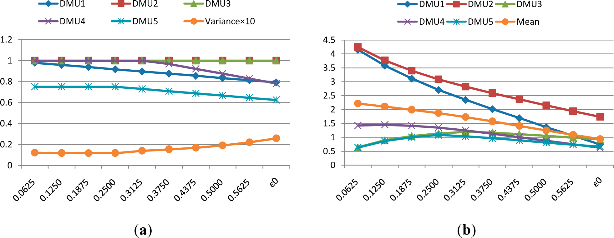
Figure 1(a) shows the different CCR efficiency of DMUs under different weight restrictions. The variance of efficient scores is also provided. As it can be seen, the DEA model is more powerful in discriminating DMUs when the weight restriction becomes bigger. In
Figure 1(b), the Euclidean distance between optimal weights and common weights are provided under different weight restrictions. The mean distance is also provided. It can be seen that when the weight restriction become bigger, the mean distance becomes smaller. That means, with the raising of the value of weight restriction, the optimal weights become more consistent with the common weights [
35]. As a result, in the following examples, only the maximum weight restriction ε
0 would be used.
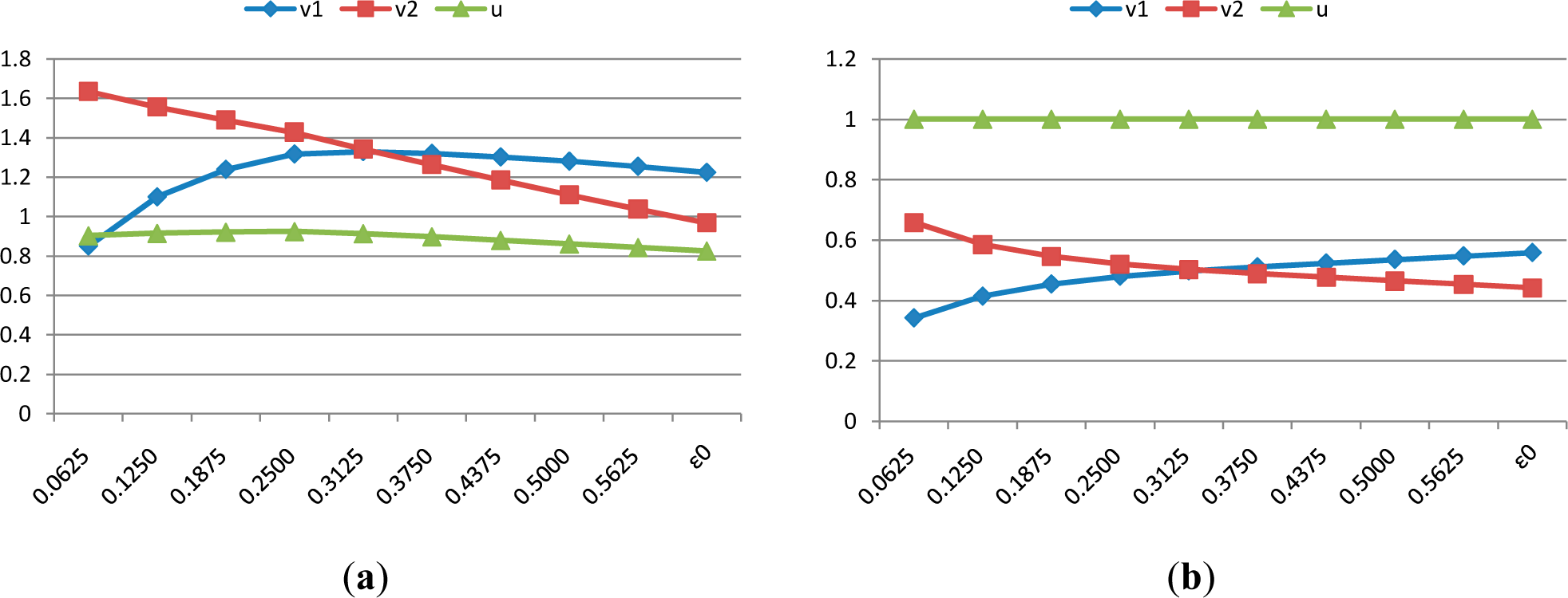
In
Figure 2, we show the different common weights under different weight restrictions. The common weights in
Figure 2(a) are the original values and
Figure 2(b) is the common weights normalized by
Equation (11). The changing tendency is clearer by the weights normalization in
Figure 2(b). Because there was only one output in example 1, the output weight would stay unchanged. With the raising of the weight restriction, the model would allocate more weight on input 1 than input 2. That is mainly because input 1 is better than input 2 for all DMUs from a global point-of-view.
Example 2. This is an artificial example with numerous inputs and outputs. By this example, we would like to show that our proposed methodology would still be effective even when the inputs and outputs are numerous. Suppose there are four DMUs with five inputs and one output, the inputs and outputs are even more than the DMUs. The input and output data is originally normalized as it is shown in
Table 6.
The computing procedure will be briefly formulated by
Tables 7~9. By solving model
(7), the maximum weight restriction is 0.2539. Then the non-zero optimal weights can be obtained in
Table 7. The normalized optimal weights are shown in
Table 8. What is more, the Shannon entropy and the importance degree of these optimal weights are provided in
Table 9. The entropy of single output is also defined as 0. The final common weights in this example are
v1 = 0.2539,
v2 = 0.2539,
v3 = 0.5816,
v4 = 0.3333,
v5 = 0.6969 and
u1 = 0.8014. Then the efficiency evaluation results by different models can be got in
Table 10.
By the comparison in
Table 10, all these four DMUs are CCR efficient. That is mainly because the inputs and outputs are too numerous, even more than the DMUs. In this situation, the traditional DEA models would be unable to discriminate or evaluate DMUs. By using the existent common weights DEA models
(3)~
(5), there are still some DMUs cannot be discriminated, such as DMU1 and DMU2. As a comparison, a full ranking of all DMUs can be got by our proposed methodology. And DMU1 has been evaluated as the most efficient DMU, while DMU4 is the most inefficient one. Our proposed method is still powerful and effective even in the numerous inputs and outputs situation.
Example 3. This real data example is selected from Chang and Chen [
40], and there are 10 Asian lead frame firms considered as the DMUs with two inputs and two outputs. The inputs are book value of tooling in 10
5 dollars (Input 1) and cost of goods sold in 10
6 dollars (Input 2). The outputs are sales revenue in 10
6 dollars (Output 1) and average yield rate (Output 2). The input and output data is provided in
Table 11.
By the application of our proposed methodology, the maximum weight restriction is 0.1244 and then the non-zero optimal weights and the normalized optimal weights can be got in
Table 12. Then the Shannon entropy of these normalized optimal weights is calculated in
Table 13. It can be seen that DMU10 has got the biggest Shannon’s entropy in inputs while DMU9 has the biggest outputs Shannon’s entropy. Then the importance degree of the optimal weights from different DMUs can be got, as it is shown in
Table 13. Based on the importance degree in
Table 13, the common weights for Example 3 are
v1 = 4.9779,
v2 = 2.2114,
u1 = 1.0654 and
u2 = 0.3539. Then the efficiency evaluation result based on out proposed methodology is provided in
Table 14. Besides the evaluation results by some other models are also provided for a comparison.
In
Table 14, there are some differences in the efficiency evaluation results. However we would like to say that our proposed methodology is more accordant with the CCR model considering the most efficient DMU and the most inefficient DMU. Although the most efficient DMUs in models
(3)~
(5) are also CCR efficient, their most inefficient DMUs are not accordant with the CCR model. As a comparison, DMU2 is evaluated as the most efficient DMU by our proposed method which is also CCR efficient. What is more, DMU9 is evaluated as the most inefficient DMU by our proposed method which is also the most inefficient in the CCR model. In other words, our proposed method keeps in accordance with the basic concept of the original DEA methodology. Besides, we also calculated the correlation coefficient between our proposed model and the existent models. And the correlation coefficients are 0.4838, 0.4690, 0.1905 and 0.3936 with the CCR model, model
(3), model
(4) and model
(5) respectively. And it can be seen that our proposed model has got the biggest correlation coefficient with the original CCR model.
Example 4. This is another real data example selected from Shakouri
et al. [
33]. As it is mentioned in [
33], the original inputs and outputs in this example are too numerous and Shakouri
et al. [
33] proposed some transformation on the inputs and outputs before efficiency evaluation. In this example, four energy technologies are considered as the DMUs with five inputs and three outputs. These four technologies are: Nuclear energy, light water reactor power plant (LWR); Nuclear energy, light water reactor power plant with reprocessing (LWRP); Fossil fuel energy, Integrated Gasification Combined Cycle power plant (IGCC); and Fossil fuel energy, IGCC power plant with CCS: 90% of CO
2 capturing (IGCCS). The inputs include: primary energy source (PES/kg), material (M/kg), labor (L/h), electric power capacity (PC/KW), total internal energy (TIE/Gj). While the outputs include: radioactive wastes (RW/kg
−1), CO
2 emissions (CO
2/kg
−1) and output energy (OE/GWh). The detailed description can be found in [
33] and the input and output data is provided in
Table 15.
The computing procedure of this example is formulated in
Tables 16~19. By our proposed methodology the maximum weight restriction is 0.2823. And the common weights for this example are
v1 = 0.3983,
v2 = 0.2823,
v3 = 0.2823,
v4 = 0.4748,
v5 = 1.1022 and
u1 = 0.2949,
u2 = 0.6850
u3 = 0.3770. The efficiency evaluation results from different models are provided in
Table 20 as a comparison.
As it is shown in
Table 20, our proposed model is still able to propose a full ranking of all DMUs even when the inputs and outputs are numerous. By our proposed model, IGCC is evaluated as the most efficient technology while IGCCS is the most inefficient one. This result is accordant with the original CCR model and also with the other common weights model
(3) and
(5). It should be noted that, any transformation on the inputs or outputs would affect the evaluation results. That would be the reason why we have got a different result with [
33]. It also should be noted that the main purpose of introducing this example is to examine the discrimination power of our model in the extreme case with numerous inputs and outputs. And the comparison in
Table 20 would be adequate for this purpose.
Therefore we can say that our proposed methodology is more powerful in discriminating DMUs while keeping the property of the basic DEA methodology. The validity and effectiveness of our proposed methodology has been proved.


