1. Introduction
Over the last twenty years, advances both in computational techniques and in non-linear dynamics have fostered a revolution in neuroscience. For the first time, it has been possible to analyze the
functional connectivity of the brain,
i.e., how pairs of brain regions collaboratively compute information, by analyzing how their respective dynamics are related. More recently, it has been realized that connectivity patterns form networks with structure at all scales, and whose properties are to some extent independent of the identity of its component nodes and edges [
1].
Of the aspects of network structural properties that most attention have received in the last years, a special position should be granted to
motifs. Motifs are patterns of connectivity involving a small number of nodes, occurring with a significantly higher frequency than expected in randomized networks [
2]. Networks of synaptic connections between neurons have been shown to exhibit network motifs. Neural circuitry has been shown to be characterized by triplets of neurons connected as feedforward loops. For instance, it has been shown that the synaptic network of Caenorhabditis elegans shows a wide repertoire of motifs [
3]. Electrical measurements of neuron tetrads showed that mammalian neuronal networks also display significant network motifs [
4,
5].
Studies of genetic regulatory networks suggest that motifs may be associated with specific functions, as memories or filters [
6–
8]. Likewise, neural motifs have been associated with an efficient integration of information [
3], and simulations suggest that they may form the building blocks of fundamental aspects of brain dynamics and function [
9].
Reference [
3] proposed a distinction between structural and functional motifs, wherein structural motifs form the physical substrate for a repertoire of distinct functional modes of information processing that can potentially engage in a context-spefic fashion in different patterns of interactions [
3]. Non-invasive electro or magnetoencephalographic recordings do not faithfully mirror the underlying anatomical circuits, so that the relationship between structural and functional networks is lost. While the interpretation of functional motifs in terms of computational units may then be lost, recent findings associating the presence of certain functional motifs with the appearance of pathological conditions [
10] suggest that functional networks built using scalp-recorded EEG or MEG devices may still retain some important physiological meaning.
Motifs are typically constructed by averaging the connectivity of triplets of nodes over long time windows, This analysis disregards motifs’ temporal evolution and only yields a single motif per triplet, so that motifs can only be counted. However, brain activity is characterized by the constant formation and destruction of couplings between distant brain regions. In the study of the brain, as well as of other real-world systems, motifs dynamics can encode important information that should not be discarded.
In this contribution, we propose a method for analyzing the coordinated dynamics of triplets of brain regions, which involves generalizing the concept of three-node motifs, and characterizing their temporal evolution using symbolic analysis.
2. Method
Given a set of
n time series
ti (
i ∈ [1,
n]), recorded by a set of
n sensors (e.g., electro- or magneto-encephalography, functional magnetic resonance imaging,
etc.), which for the sake of simplicity, are suppose to all be of the same length, denoted by
l, the first step in motif characterisation consists in selecting three sensors (nodes),
i.e.,
n1,
n2 and
n3. Notice that this process can be generalized to an arbitrary number of sensors (nodes), in order to obtain higher order motifs. The corresponding three time series (
,
and
) are divided into non-overlapping windows to length
τ—see the upper part of
Figure 1 for a graphical example. These three fragments are then mapped into a motif, by calculating the synchronization level between pairs of sensors, and activating the corresponding link when such synchronization exceedes a threshold
ρ. Notice that, at this point, the three time series are transformed into a sequence of motifs, which can be understood as a time evolving [
11] or multi-layer network [
12]. Finally, the time evolution of such motifs is analyzed by means of symbolic analysis. Specifically, each possible motif is associated to a symbol—bottom part of
Figure 1. Several techniques are available to analyze the appearance frequency of such symbols [
13–
15]; here we use the following two methods:
A high entropy, and consequently a low number of forbidden motifs, implies that the corresponding triplet of sensors is showing a high variability in its dynamics and connectivity pattern. On the other hand, the presence of a fixed motif, and thus of minimal entropy, suggests that the dynamics of the triplet does not evolve with time.
The goal of this methodology is ultimately two-fold. Firstly, by studying the evolution of the entropy as a function of the applied threshold ρ, it is possible to estimate the synchronization level that is optimal to obtain the richer dinamycs in the triplet. Secondly, an analysis of the entropy obtained for different time windows τ yields information about the characteristic time scale at which such dynamics develop.
Furthermore, the methodology presented here extends and merges two different approaches used in the study of brain dynamics. First, while in the original definition of a motif, its component nodes need to be connected [
2], here we consider any possible pattern of connectivity among nodes, including disconnected graphs. Second, the analysis of the time evolution of motifs is performed in a way similar to the ordinal patterns methodology proposed by Bandt and Pompe for the analysis of univariate time series [
16,
17]. Instead of creating symbols from the evolution of a given observable through time, here each symbol represents the evolution through space, specifically through the space created by the different triplets of observables.
3. Data Set Description
Resting brain electrical activity was recorded from eight healthy volunteers under two conditions, eyes closed and open. Each condition lasted 24 s. A standard 56 electrode montage, with electrodes positioned according to the extended 10 – 20 System location, with a nasion reference was used. The electro-oculogram was also recorded, for blink, vertical, and horizontal eye movement correction [
18]. The EEG was amplified (0.05 – 100 Hz) and digitized at 500 Hz.
A Pearson’s linear correlation was used to calculate the synchronization level between pairs of time series. While more complex metrics can be used, e.g., non-linear measures like Synchronization Likelihood [
19], or causality measures like Granger Causality [
20] or Transfer Entropy [
21], here linear correlation was selected for its simplicity and low computational cost.
4. Entropy and Thresholds
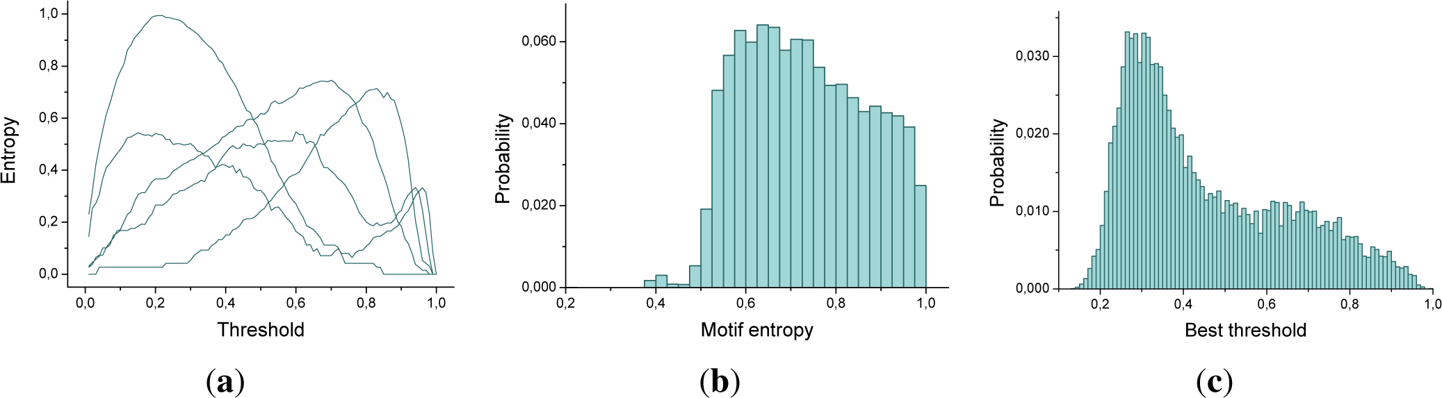
Recalling that entropy represents the variability in the motifs within each triplet of sensors, an entropy close to zero implies that just one motif can appear. This is indeed the situation corresponding to extremely high (low) values of ρ, which always result in a completely disconnected (completely connected) motif. On the other hand, a high entropy should be expected between those extrema, indicating a rich neural dynamics.
Figure 2a depicts the evolution of the entropy as a function of the threshold applied for 5 triplets of nodes, for a large time window length (
τ = 60). It can be appreciated that a maximum is indeed observed, although for each one of the triplets this corresponds to a different
ρ.
Figure 2b and c also respectively reports the histograms for the entropy and the optimal threshold for all the 175.616 triplets of sensors corresponding to a subject. Here, and in what follows, by optimal threshold we refer to the threshold that maximizes the motif entropy.
The most important conclusion that can be drawn from
Figure 2 is that each triplet of sensors has to be associated to a different threshold, in order to maximize the information codified in its associated motifs. Furthermore, there is an important variability in such thresholds: while most of the triplets benefit from a low threshold (
ρ ≈ 0.3), a non-neglibible fraction requires
ρ > 0.8.
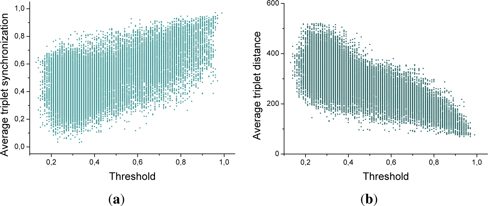
It is clear that such variability may be due to volume conduction. Specifically, triplets of neighboring sensors are usually associated with higher correlations; therefore, it may be expected that, in such situations, a higher threshold is required to discriminate the additional synchronization caused by shared information processing. This is confirmed by an analysis of the correlation between the best threshold on the one hand, and the physical distance and synchronization level between the three sensors on the other—see
Table 1 and
Figure 3.
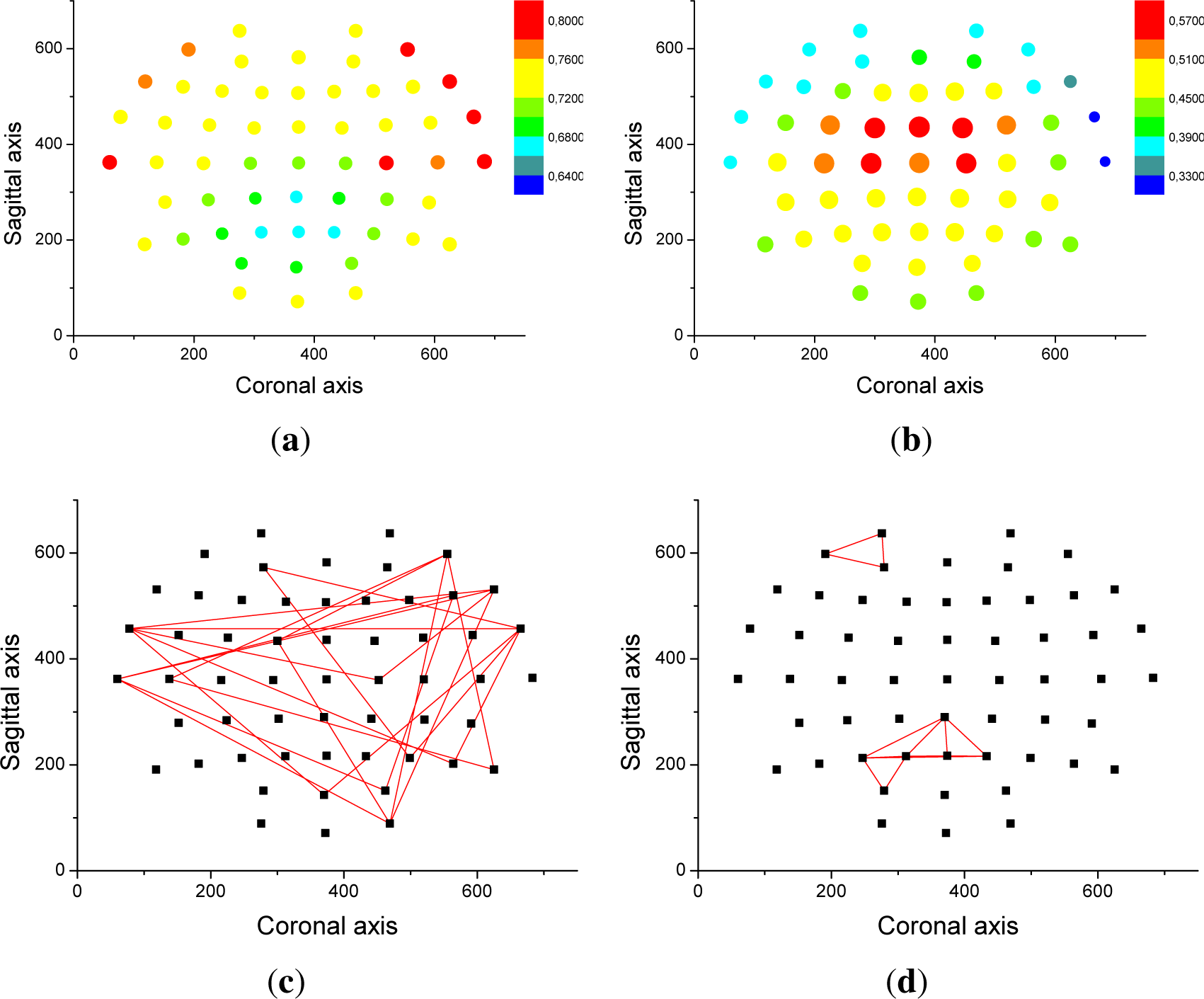
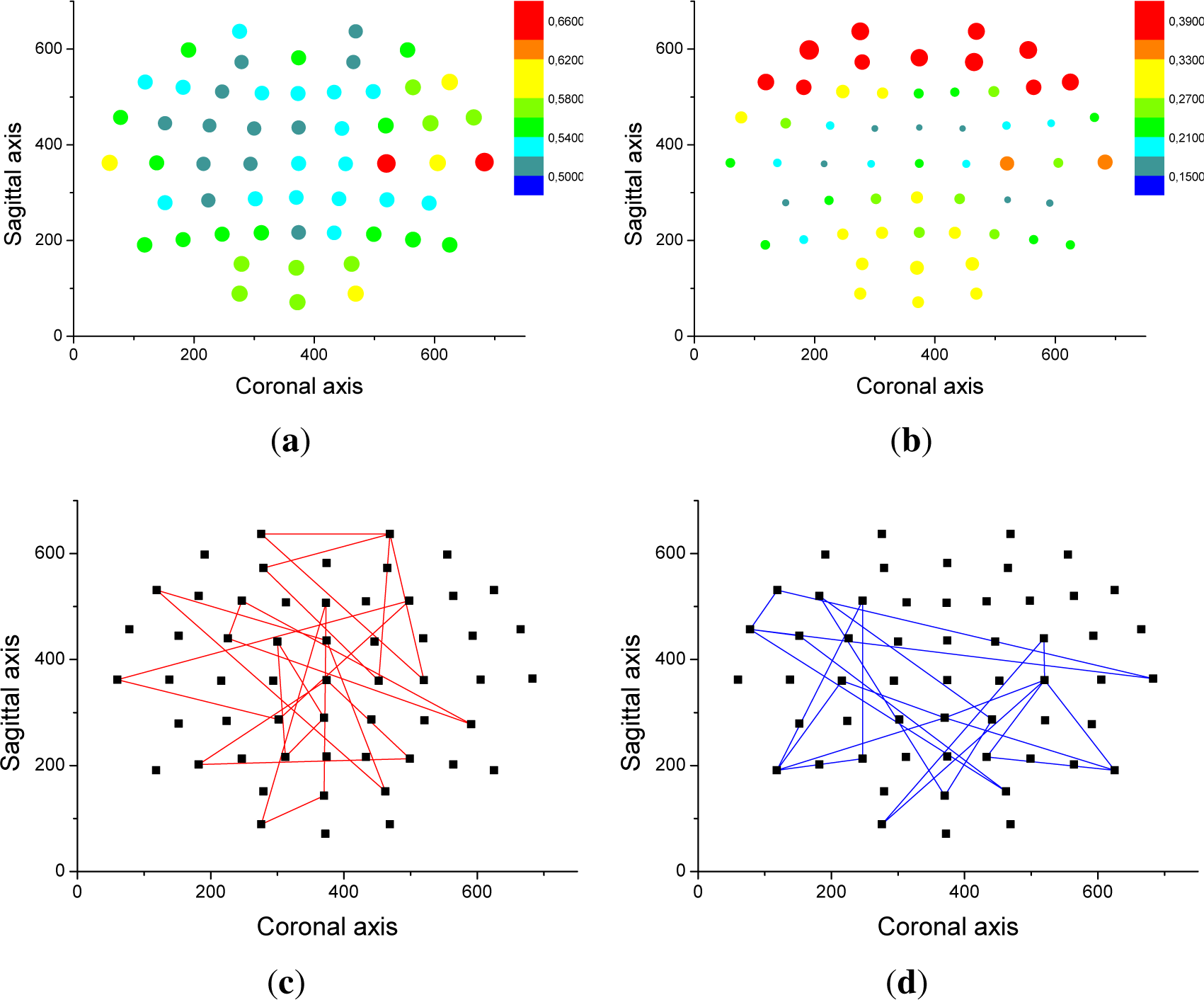
From an analysis of the correlation results, it appears that only half of the value of the optimal threshold can be explained by volume conduction. In order to explain the source of the other half,
Figure 4 depicts the relationship between entropy and the spatial position of nodes. Specifically, the color and size of each dot in
Figure 4a,b represent the average entropy and optimal threshold of all triplets to which a given node belongs. Frontal and frontal-temporal electrodes are associated with high entropies and low thresholds, while the opposite holds for parietal electrodes. Additionally,
Figure 4c,d report the eight triplets that are associated with the highest entropy and highest threshold.
Finally, it is worth analyzing if any additional information is obtained by using the number of
forbidden motifs, instead of the motif entropy, in order to estimate the best threshold, in a way similar to what usually performed in time series analysis through the Bandt and Pompe methodology [
17]. In this case, the optimal threshold corresponds to the one that minimizes the number of forbidden patterns. The correlation between the best thresholds obtained in both cases, 0.5623, indicates that both approaches are qualitatively similar. Furthermore, a high correlation is obtained between the entropies obtained in both cases,
i.e., 0.7781. Due to this similarity, in what follows, only results corresponding to thresholds maximizing the entropy are presented.
5. Entropy and Time Scales
Once the best threshold has been defined for each triplet of sensors, it is possible to analyze the evolution of the entropy as a function of the time window length
τ.
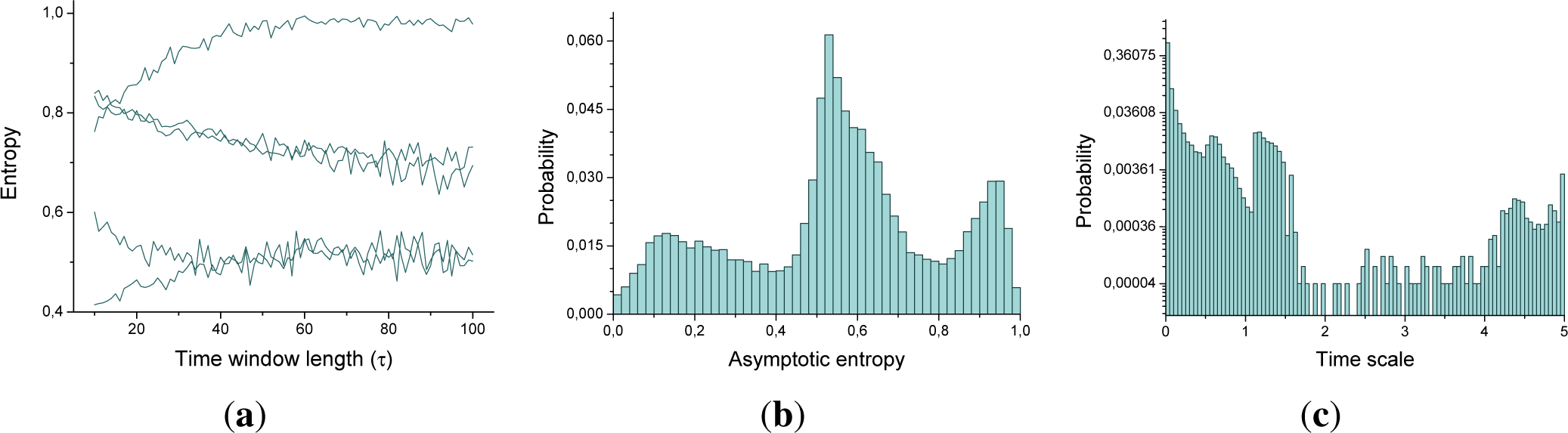
Figure 5a reports such evolution for five triplets of nodes. It can be appreciated that the value of the entropy changes, from low to high
τ s, until an asymptotic value is reached. In order to model this dynamics, the evolution of the entropy of each triplet has been adjusted to the following exponential function:
Therefore,
α represents the asymptotic entropy value,
i.e., the characteristic entropy of the triplet after the initial transient. Furthermore,
γ represents the characteristic time scale of the triplet, so that the higher the value, the faster the triplet reaches its steady state.
Figure 5b,c report the two histograms corresponding to
α and
γ for all triplets of a single subject. A great variability can be observed, especially in the time scale: while most of the triplets have a slow evolution, some of them reach a steady state with a time window of less than 20 samples.
In a way similar to
Figure 4,
Figure 6 depicts the spatial information related to the asymptotic entropy and time scale of motifs. Specifically, the color and size of each dot in
Figure 6a,b represent the average aymptotic entropy and time scale of all triplets in which that given node participates. Furthermore,
Figure 6c,d report the eight triplets that are associated with the fastest and slowest time scale. As in
Figure 4, nodes in the frontal and frontal-temporal regions seems to be associated to a specific dynamics, in this case a very fast time scale. These results are in partial agreement with findings from a recent study using fMRI, where the orbito-frontal limbic module was found to be more dynamic whereas the visual, default mode and somatomotor modules were found to be more static [
22]. Additionally, the heterogeneity in the motif time scales suggests that changes in functional connectivity do not occur en masse [
22], but instead in an asynchronous manner across the scalp.
6. Extending Motif Entropy
The concept of motif entropy described here can be extended in several ways: this Section aims at describing some of them, in order to highlight the flexibility and generality of the proposed concept.
First of all, up until now motifs were created using binary values,
i.e., links can either exist (whenever the absolute value of the correlation is above a given threshold) or be absent—see
Figure 1. When the sign of the correlation is not discarded, the result is the creation of
signed motifs [
23],
i.e., motifs whose links can assume three states: [0, +, −]. This should, in principle, allow to describe more complex phenomena in brain dynamics, as for instance
relay synchronization [
24]. The entropy of the symbolic dynamics of these signed motifs can be calculated using
Equation (1), taking into account that there are now 27, as opposed to 8, possible motifs.
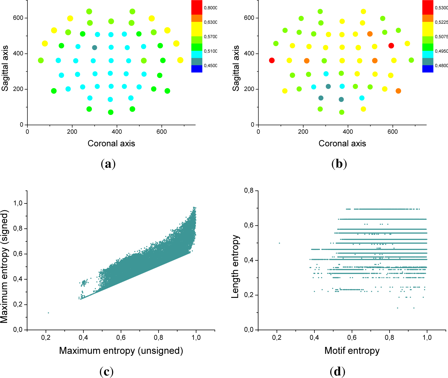
Figure 7a confirms that the frontal region is characterized by a higher entropy, and therefore by a richer dynamics. Furthermore,
Figure 7c presents a scatter plot of the signed motif entropy, as a function of the entropy previously found for each triplet of sensors.
Besides the probability distribution of motifs, i.e., the probability with which they appear in the time series, one may be interested in the distribution of their lengths, that is, whether they are stable or only appear for short period of times. To this end, one can calculate the average number of times a motif i sequentially appears (li), and calculate the associated entropy as:
pt being the fraction of motifs with
l =
t. The higher
El, the more heterogeneous the motifs length: some of them may only appear in short bursts, while other may have a higher stability.
Figure 7b and d respectively represents the average length entropy for each EEG sensor, and the scatter plot of the length entropy, as a function of the entropy of each triplet of sensors. It can be seen that
El and
E are not correlated, indicating that
El provides complementary information about the brain dynamics.
Finally, two other extensions can be analyzed. First, the correlation between consecutive motifs, i.e., the entropy of the matrix ε whose element (i, j) indicates the probability of finding motif i at time t and motif j at time t + 1. One may also calculate motifs with different number of nodes, e.g., 2, 4, etc. Nevertheless, it should be noticed that the entropy associated with pairs of nodes has little interest, as a threshold can always be found that maximizes the entropy (i.e., that balances the appearance and disappearance of a single link).
7. Inter- and Intra-Subject Variability
In order to complete the assessment of the characteristics of the entropy associated to motifs, it is necessary to ascertain the variability associated with each of the described metrics, i.e., optimal thresholds, asymptotic entropy and motif time scales. This may help clarifying two points. On the one hand, if inter-subject variability is low, e.g., the best threshold is constant for all available subjects, this would represent a common feature among different individuals, related with the way the brain processes information. On the other hand, even for high inter-subject variability, a low intra-subject variability would imply that motifs dynamics could be used as a personal fingerprint of the information processing style of each subject.
To address these points, we considered all eight available subjects. Two recordings in two different conditions, eyes opened and closed, were available for each of them, for a total of 16 sets of EEG signals. For each of these sets, the previously described metrics were extracted for all 175.616 triplets of sensors available: optimal thresholds, asymptotic entropy and motif time scales. Inter and intra-subject variability was estimated using the Pearson’s linear correlation.
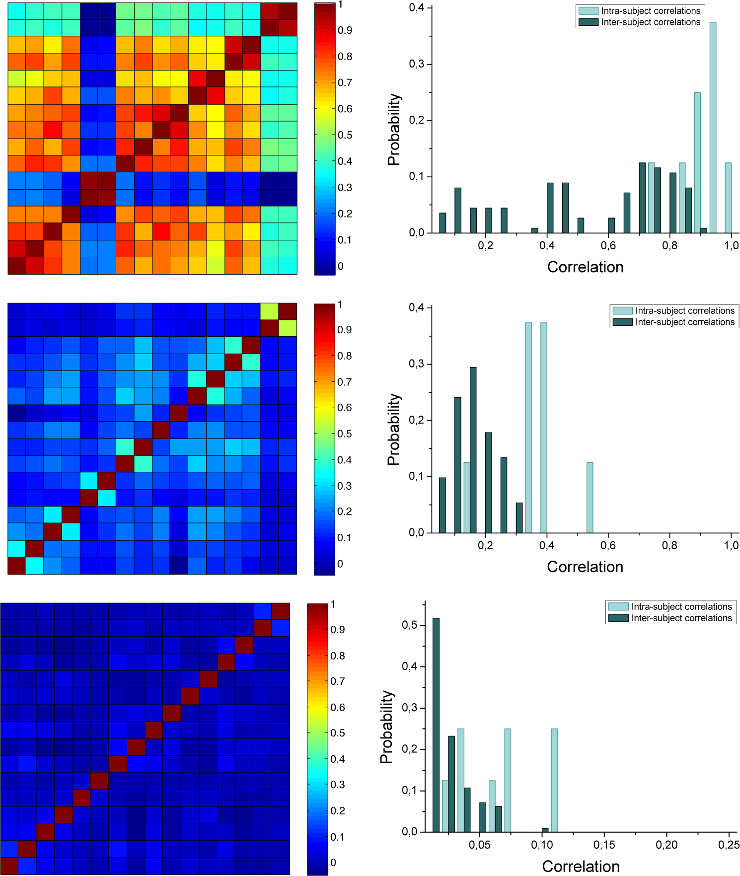
Figure 8 reports the obtained results. Graphs on the left side report the pairwise correlations for the 16 conditions. The two conditions of each subject are grouped together:
i.e., the first two rows and columns correspond to subject 1, the third and fourth to subject 2, and so forth. The same information is also presented in the right panels, as probability histograms. Top, center and bottom panels respectively correspond to the optimal thresholds, asymptotic entropy and motif time scales.
Two main conclusions can be drawn from
Figure 8. Firstly, there is a high inter-subject variability, as shown by the fact that the inter-subject correlations are always below 0.4 both for the asymptotic entropy and the time scales. Interestingly, the inter-subject correlation corresponding to the optimal threshold is significantly high, except for subjects 3 and 8. As no additional information is available about these two subjects, we cannot know the cause for such difference. Secondly, the intra-subject variability is always lower than the inter-subject one, as indicated by the higher correlation coefficient, suggesting that motifs, and their entropies, may be thought of as subjective brain dynamics fingerprints, irrespective of the condition under which the EEG recording has been made. We note however that these results should be taken with some caution until they are confirmed with a larger population sample and more general experimental conditions.
8. Conclusions
In this contribution, we define a methodology for calculating the entropy corresponding to the dynamics of three-node motifs, based on symbolic analysis. The usefulness of this approach is demonstrated through the study of functional brain activity at rest as measured by EEG. Our results showed each triplet of sensors had a characteristic time scale and synchronization threshold associated with the appearance of functional structure, and that motifs had a topographically specific distribution. Motifs varied widely across subjects, but for each subject, their time scales and thresholds were robust with respect to the experimental condition, suggesting that they may represent a subject-specific dynamical signature.
While scalp EEG motifs are not liable to a direct interpretation in computational terms, but only in terms of coordinated activity across brain regions, our method captures the extent to which these patterns are stable in time. Our results suggest that each motif found in the broadband signal of the EEG has its own time scale, sometimes much faster than alpha band ones (∼ 10 Hz) which dominate resting brain activity, the relationship of which with the oscillation frequency of the component electrodes will need to be clarified.
On the other hand, while the significance of the topographical characteristics of motifs’ time scales found in our study should be taken with some caution, given the sample size of our population, the abundance and speed of motifs at frontal electrodes may be consistent with the speficic information integration and executive role of the underlying brain regions.
From a methodological view-point, the time-scale and threshold heterogeneity across motifs indicates that the analysis of motifs cannot be done in a collective way; instead, each motif should be studied separately, using it optimal τ and ρ. More generally, our results point to a complex role of thresholds in network reconstruction. While thresholds are typically chosen once and for all in most network reconstruction studies, each threshold uncovers specific structural aspects of brain activity, so that network analysis should find out the ones that capture fundamental information in a context-specific way.
Finally, the interested reader can find an open-source MATLAB source code for the computation of the motif entropy at [
25].


