1. Introduction
A reliable rating curve at a river site is of fundamental importance in hydrological practice, as accurate discharge values are fundamental in addressing water resources management and rainfall-runoff model calibration as well as hydraulic risk assessment. These topics might be seriously affected by uncertainty if the stage-discharge relationship is poorly estimated at river gauging sites. One of the main issues is often the lack of streamflow measurements at high stages. At gauged river sections flow data needed for rating curve estimation are often limited to low flow stages. This is due to the difficulty and dangers that operators have to face to sample velocity points in the lower portion of the flow area during high floods in particular when classical propeller current meters are used. Recently, the introduction of Acoustic Doppler Current Profilers (ADCP) installed on moving-vessels has allowed operators to address the above mentioned problems even if several limitations remain. Indeed, during high floods any increase in sediment transport produces a reduction of the signal-noise ratio of acoustic sensors [
1] along with the capability of the signal to penetrate through the water. In addition, high flow conditions are often characterized by high water depth, high velocity and high turbulence that can affect the water depth estimation because of roll and pitch motions of the vessel [
2] as well as vessel tracking [
3]. Moreover, due to high velocity and high water levels, branches or entire trunks of trees can be suspended by the current and could represent a risk for the instrument and operator.
To overcome these problems, a consistent approach considers the correlation between mean flow velocity,
um, and the maximum one,
umax, which is easily sampled as it is located in the upper portion of flow area. Entropy theory [
4] shows that
umax is strictly linked to the mean flow velocity,
um, through a linear entropic relationship based on a single parameter,
M, which is a characteristic of the gauged river site in particular [
5,
6], and also of the river in general [
7]. Therefore by sampling
umax, the information on
um (and hence on discharge) can be inferred also for high flows in situations where the flow area is known. The considerable benefit of using
umax during flow measurements is that high flows can be more readily monitored, making the measurement less time consuming and safer for the operators and instruments. In fact, maximum velocity can be determined using conventional devices, such as current-meters or acoustic sensors, or using more recent radar devices for surface velocity monitoring. In the first case, the sampling concerns only a small part of flow area so that it is possible to minimize the sampling time and the contact with the surface water. In the second case, the velocity measure is obtained without any contact and safety conditions [
8,
9]. Moreover, recent developments in Interferometric Synthetic Aperture Radar (InSAR) techniques make possible new scenarios where the river surface velocity can be inferred from space. InSAR techniques allow sensing river surface velocity in the direction orthogonal to the sensor track, called radial velocity. This feature was already tested on the tidal extent of the Elbe river using TerraSAR-X satellite [
10,
11] with an average accuracy of 0.1 m/s while the hydrological community is waiting for the data of the current airborne mission AirSWOT [
12]. This mission will test, calibrate and validate the instrument of the next satellite mission SWOT. The KaSPAR sensor [
13], used in AirSWOT, was designed to provide not only elevation mapping but also radial velocity information about the surface [
13]. Retrieval of water surface velocity from satellite or airborne sensors coupled with the entropy based method could make a near global driver discharge monitoring very possible in the near future.
Nevertheless, entropy based methods [
4–
6,
14,
15] require the knowledge of the
M parameter that is usually estimated by linear regression using the historical database of maximum and mean velocity pairs. The database is often built on the basis of data acquired during stream flow measurements carried out by using standard procedures for sampling velocity points in the flow area. In most cases, these procedures are based on one point, two points or three-points methods [
16–
18] and for which no information on
umax is given. By using the velocity entropy profile, Chen and Chiu [
14] inferred
umax from the velocity information using two points methods. However, the position of
umax in the river cross section, in terms of both span-wise location and depth, needs to be well detected.
Another possibility is to estimate
M by using one of the approaches proposed by Farina et al. [
19]. These approaches are based on different levels of knowledge of the velocity field consisting of (i) the entire spatial distribution of velocity in the flow area, (ii) the surface velocity distribution and (iii) the sole sampling of
umax. In this latter case, the assumption on the surface velocity distribution may influence the accuracy of the
M estimate [
19]
.For a gauged site with an existing database, an alternative could be to try to recover the available information and fill the gap concerning
umax. Satisfactory results are achieved with standard methods for low and medium flows [
20], allowing the collection of data that could have value for the discharge estimation during high flow and then for the rating curve extrapolation beyond the velocity measurement field. To this end, the friction-slope method would be suitable [
16]. This method is based on the Manning equation and in particular on the friction-slope parameter,
α, representing the ratio between the square root of the energy slope and the Manning roughness coefficient [
16]. For steady flows, with increasing water levels,
α tends to an asymptotic value α
∞ [
21], which can be used for discharge extrapolation. Even though the parameter
α may be affected by uncertainty during unsteady flows, it might be useful to address velocity measurements during high flows recovering the historical information provided by standard methods. This can be achieved by investigating if a correlation between α and the entropic parameter
M holds and if this correlation can be used to update the historical information with new measurements. This is of considerable interest from a hydrological practice point of view, as the gauged river sites where these methods are applied to monitor the flow velocity,
umax is not known and as a consequence the entropy parameter,
M, cannot be assessed. To this end the target of this work is twofold:
- (1)
to detect a possible relation between M and the parameter α at a river site. In order to achieve this a stream flow database built on velocity point methods is used;
- (2)
to propose a methodology to estimate M from α values obtained with standard velocity measurements wherein umax was not sampled.
The novelty of the proposed approach to estimate of M is down to the recovery of the available historic information at a river site even in the case the knowledge of umax is missing.
Four river gauged sites of different hydraulic and geometric characteristics are used for the analysis.
2. Standard Velocity Points Sampling Methods: A Brief Review
Traditionally, the discharge measure is obtained by spatially integrating velocity points, sampled along verticals by means of point-velocity meters [
16]. Starting from these sampled velocity values, depth averaged velocities are computed and turned into discharge by applying the “velocity-area” method [
17,
18]. The estimation of depth-averaged velocity depends on the number of sampled points per vertical and can be addressed with one of the standard methods described below. The theoretical background for these methods is given by the turbulent boundary layer theory [
20] and in particular by the so called “wall law” [
22], which represents the vertical velocity profile by means of a logarithmic law. This velocity distribution is applied to the entire water depth, even if it is strictly valid only within the boundary layer in the so called “logarithmic or inertial” sub-layer [
22]. The classical logarithmic law can be expressed as:
where:
y is the distance from the bottom;
u*, is the shear velocity,
(g is the gravitation acceleration, RH is the hydraulic radius and Sf is the energy slope);
k is the Von Karman constant;
y0 is the location where the velocity hypothetically equals zero.
On the basis of
Equation (1), the depth averaged velocity values can be estimated by sampling a few velocity points for vertical so that sampling time can be reduced.
In practice, the mean vertical velocity,
umv, can be calculated on the basis of the sampling of one, two or three velocity points per vertical profile by using the following empirical relations [
16,
18]:
where u0.2, u0.6 and u0.8 are the velocities corresponding to 0.2, 0.6 and 0.8 of the water depth, D, of the entire vertical profile. Henceforth, these methods for velocity sampling will be referred as “standard methods”.
4. Field Data
The described analysis has been carried out on the basis of available data at four gauged sites located in Italy and Algeria, whose main characteristics are summarized in
Table 1. For each gauged site, the historical velocity measurement datasets have been taken into account, for a total of more than 450 analyzed measurements, and their characteristics are summarized in
Table 2. Measurements were carried out by applying the “velocity distribution method” [
18] and using propeller current-meters. In particular, as indicated by ISO 748 [
18] a number of velocity points (enough to reconstruct the vertical velocity profile) were sampled while a number of verticals were also taken (ensuring a center-to-center distance not exceeding 2 m in the whole flow area). Exposure times of 30 s and measured velocities greater than 0.4 ms
−1 were considered. Therefore, for each velocity measurement,
umax can be assumed equal to the maximum sampled velocity [
6]. As the aim is to demonstrate the reliability of the relationship between α and Φ, it does not matter if α has been assessed by detailed velocity sampling along the vertical or using one of the standard methods.
The datasets provided values of water level and discharge, maximum and mean flow velocity, flow area and water depth. The hydraulic radius,
RH, was calculated on the basis of the available information. For the gauged sites in Italy, since topographical surveys were available,
RH was computed using the method for compound sections, assuming the hypothesis of constant energy slope across the river cross section [
27]. For the sites in Algeria no topographical surveys were available and
RH was calculated as the ratio between the values of flow area and wetted perimeter, obtained from the velocity measurement reports.
5. Results and Discussion
In order to apply the entropic model at the investigated gauged sites,
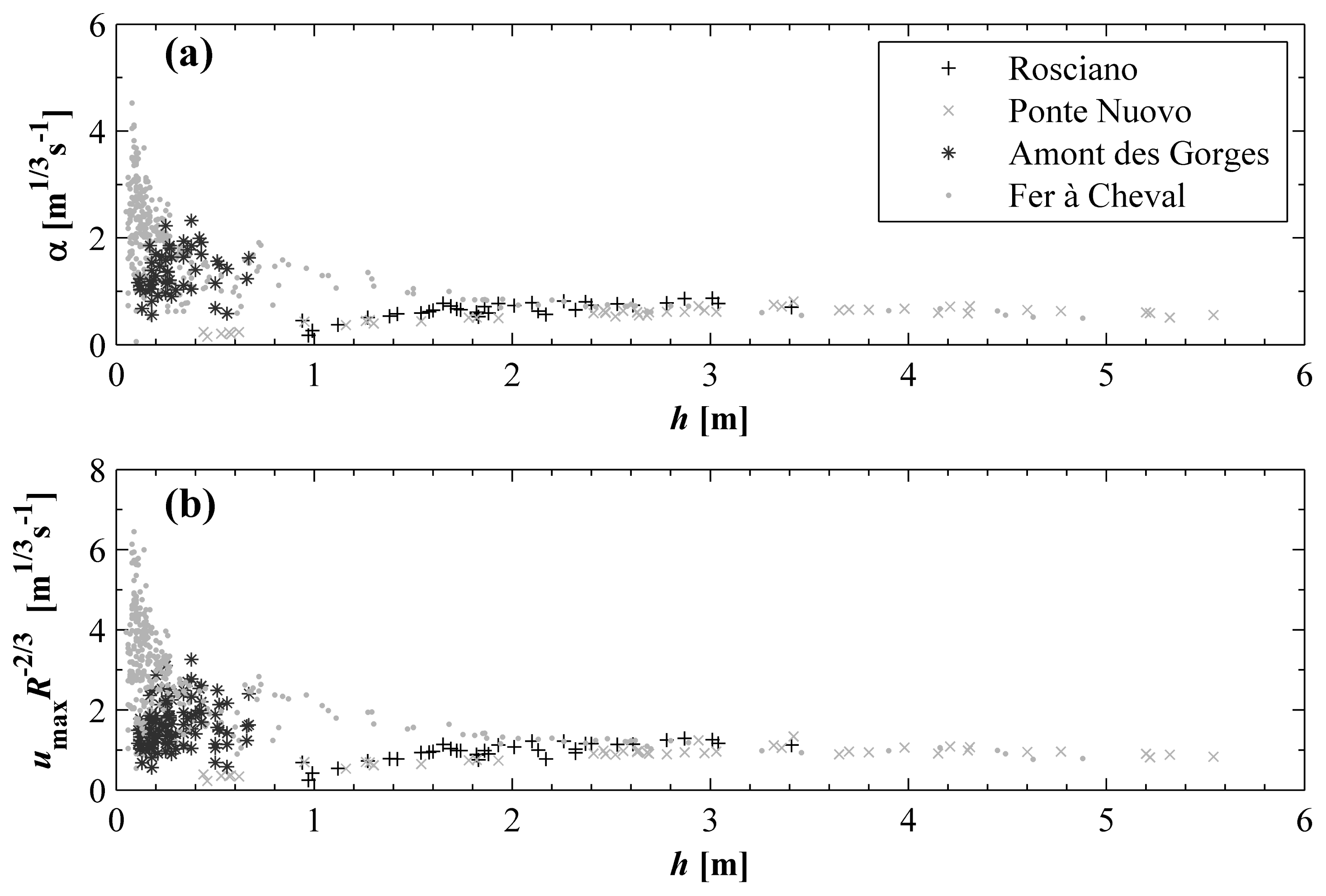
Equation (8) have to be tested. To this end, the quantities α and
umaxRH−2/3 have been plotted as a function of the water level,
h, for the four gauged sites.
Figure 1 shows the different behaviors of α and
umaxRH−2/3 for the river sites. In particular, for the river sites in Algeria,
α shows a general decreasing trend, with a significant scattering for low water levels and an asymptotic value that is quite evident at Fer à Cheval river site. By contrast, the river sites in Italy show an increasing trend of α versus
h (see
Figure 1a). The different behavior of the parameter α versus
h might be ascribed to the different hydraulic and geometric characteristics which significantly vary for the Algerian rivers, mainly in terms of roughness. Nonetheless, in all analyzed river sites the parameter α and the quantity
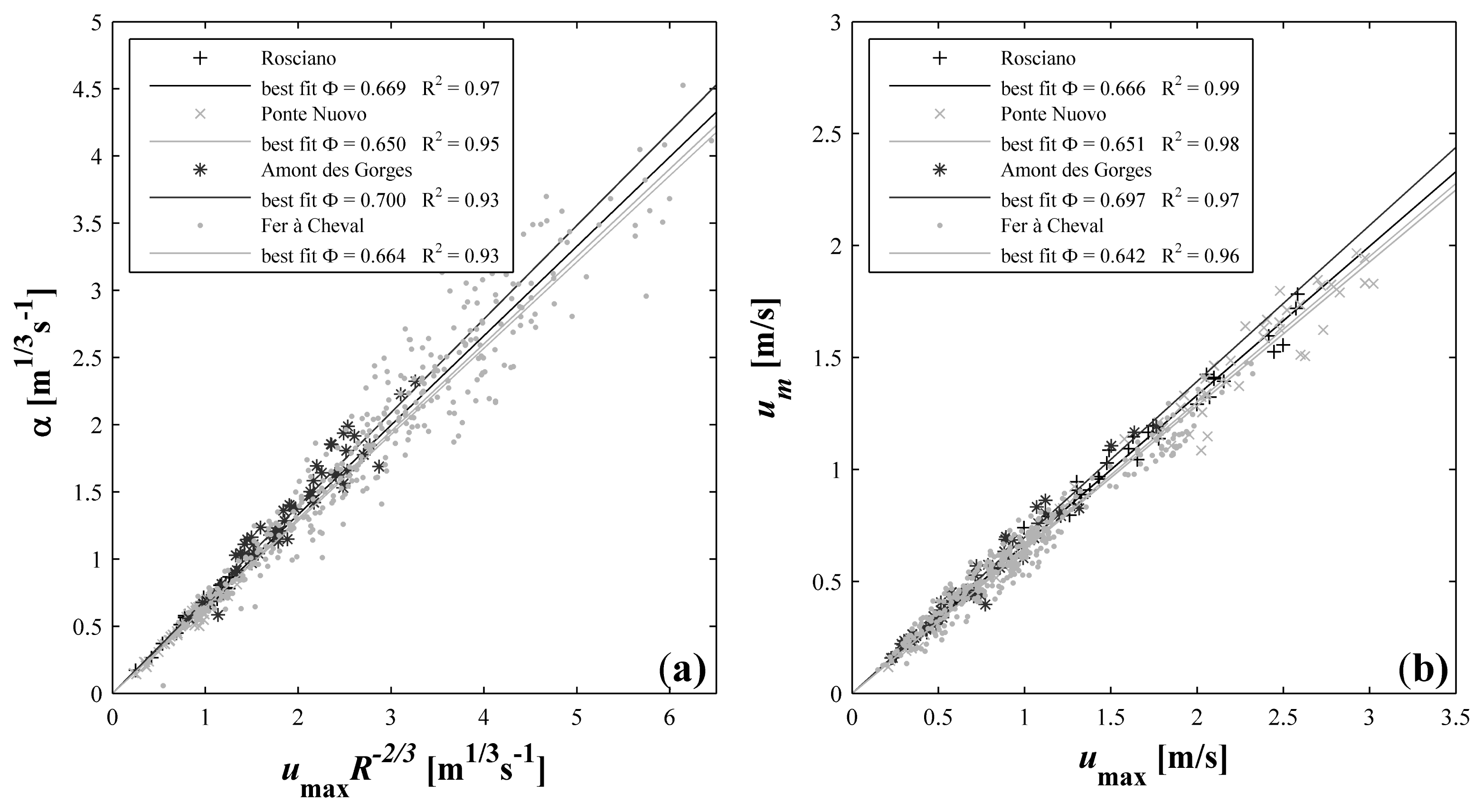
umaxRH−2/3 show a similar trend, indicating a correlation between the two quantities. This correlation is confirmed in
Figure 2a, where the trend of α versus
umaxRH−2/3 is shown along with the best fit lines, and in
Table 3, where related values of determination coefficients and Φ are listed. For comparison, the same table summarizes the Φ values obtained by (
umax, um) pairs, whose trend is illustrated in
Figure 2b for the four gauged sites. As can be seen from
Table 3, the values of Φ assessed by considering the pairs (α,
umaxR−2/3) along with (
um,
umax) are similar for all the analyzed river sites, except for Fer à Cheval, for which the Φ value estimated by (α,
umaxRH−2/3) pairs appears slightly overestimated, likely due to an overestimation of the hydraulic radius.
5.1. Estimation of Φ on the Basis of a Historical Sample of Conventional Velocity Measurements
The results illustrated in the previous section show that between the quantities α and
umaxRH−2/3 there is a linear relation, defined by
Equation (8), that can be exploited to estimate Φ. In the case of velocity measurements carried out by standard methods the maximum velocity,
umax, is generally not sampled and Φ cannot be inferred. Therefore, from a hydrological point of view it is of considerable interest to investigate the possibility of estimating Φ by integrating the information concerning α, obtained from a historical sample of standard velocity measurements, with the one related to
umaxRH−2/3, obtained sampling only
umax. In this context, to carry out new velocity measurements is feasible. In fact, on the one hand, the sampling of
umax only is not costly, considering that
umax occurs in the upper portion of the flow area [
7] and, on the other hand, the hydraulic radius,
RH, can be easily computed if the geometry of river section is known. Therefore, in order to verify the possibility of assessing Φ from α values, a backwards-testing procedure is considered. The velocity dataset of each river site is split into two consecutive periods of equal duration. In the first period, indicated as “historical”, we surmise that velocity measurements are carried out by standard methods and no information about
umax is available. For the second period, called “new”, it is assumed only
umax is measured and
RH determined by the topographical cross-section survey. In particular, considering the minimum and maximum water level,
hmin and
hmax, recorded in the dataset, in accordance with the gauged site a certain number of classes ensuring at least two measurements are identified in the range [
hmin hmax] and for that a step of flow depth 0.25 m is used. Therefore, for each class, two sets of velocity measurements are present. The first mimics the historical information obtained using standard methods and allows the estimation of α. The second set represents the “new” period of measurements where
umax is sampled thus providing the quantity
umaxRH−2/3. In other words, for each identified class of water level, the “historical” dataset provides information to estimate α values, while the “new” dataset allows the assessment of Φ values, independently from the “historical” dataset.
In each class the corresponding values of α along with those of
umaxRH−2/3 were averaged and, for each gauged site, Φ is estimated on the basis of respective pairs (α
m,
umaxRH−2/3|
m). Therefore, the backwards-testing procedure consists of verifying if the correlation (such as depicted by
Equation (8) between α and
umaxRH−2/3, obtained from the historical and new velocity data, respectively) has been achieved. If it has, at a gauged river site where only standard velocity measurements are carried out, the sampling of
umax in later periods would allow the estimation of Φ from α values and, hence, to be used to estimate the velocity measurements for high flows. However, it has to be pointed out that the procedure assumes that, on average, the flow conditions do not change over time, thus maintaining a similar velocity distribution for the same water level.
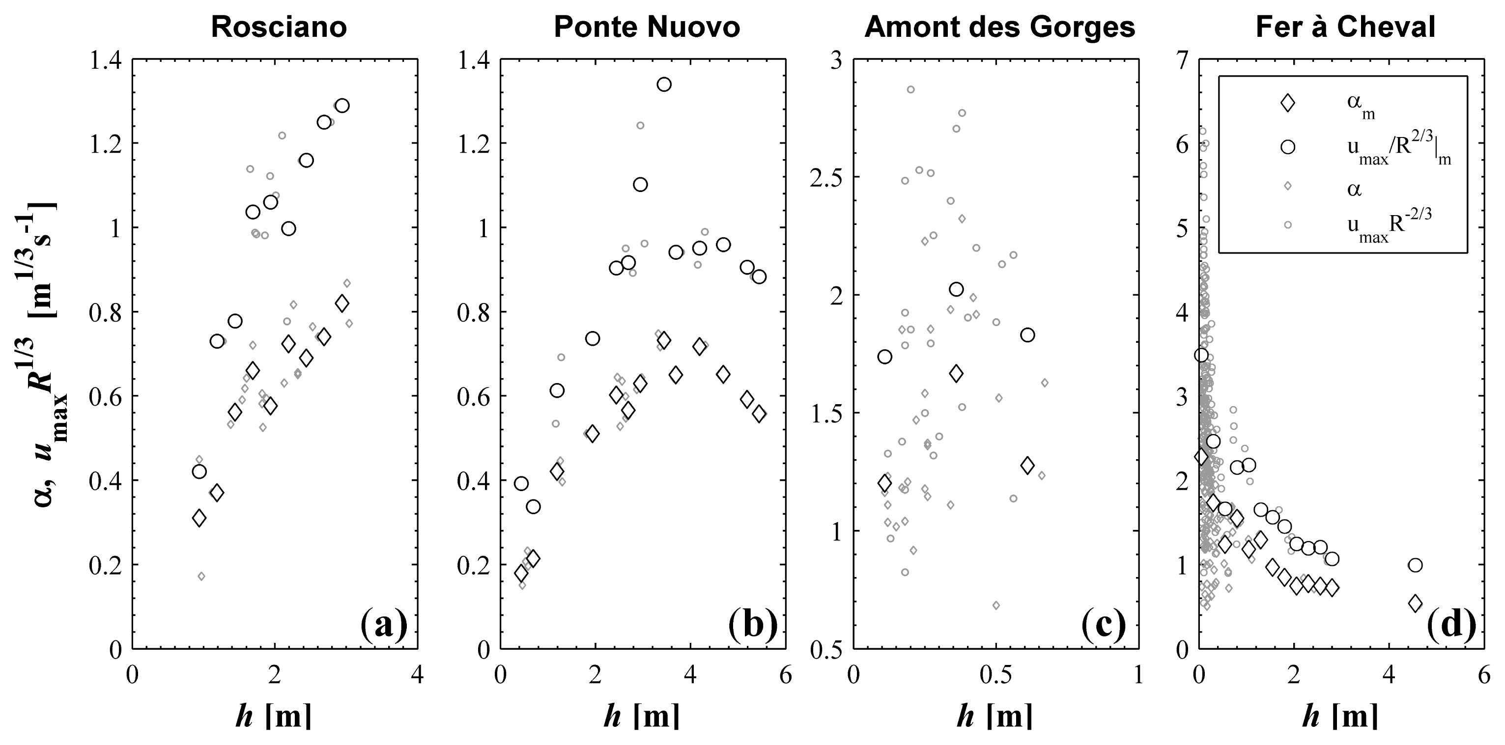
Figure 3 shows the trend of pairs (α,
umaxRH−2/3) and (α
m, [
umaxRH−2/3]|
m) as a function of water level,
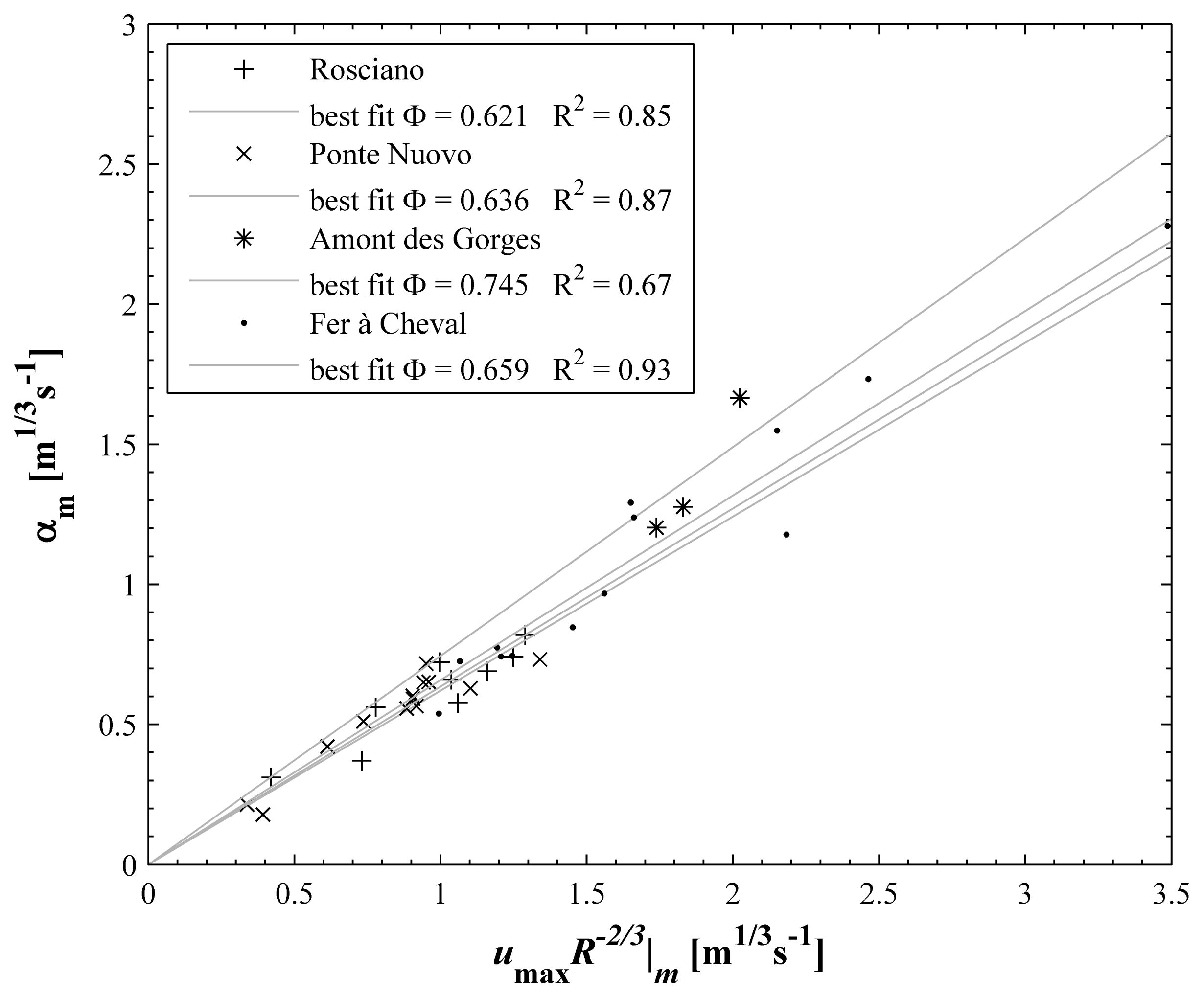
h, while in
Figure 4 the best fit lines are displayed. As can be seen in
Figure 3, both the quantities α and
umaxRH−2/3 and the related average values α
m and [
umaxRH−2/3]|
m show a similar trend versus
h and a good correlation (see
Figure 3) as also reported in
Table 4, wherein the estimated Φ values along with the corresponding determination coefficients are shown. With the exception of Amont des Gorges, where only three classes have been identified (see
Figure 3c), coefficient of determination values greater or equal than 0.85 were obtained (see
Table 4). Moreover, comparing
Table 3 and
4, no significant differences can be found between the Φ values computed following the proposed procedure (see
Figure 4 and
Table 4) and those previously obtained (see
Figure 2 and
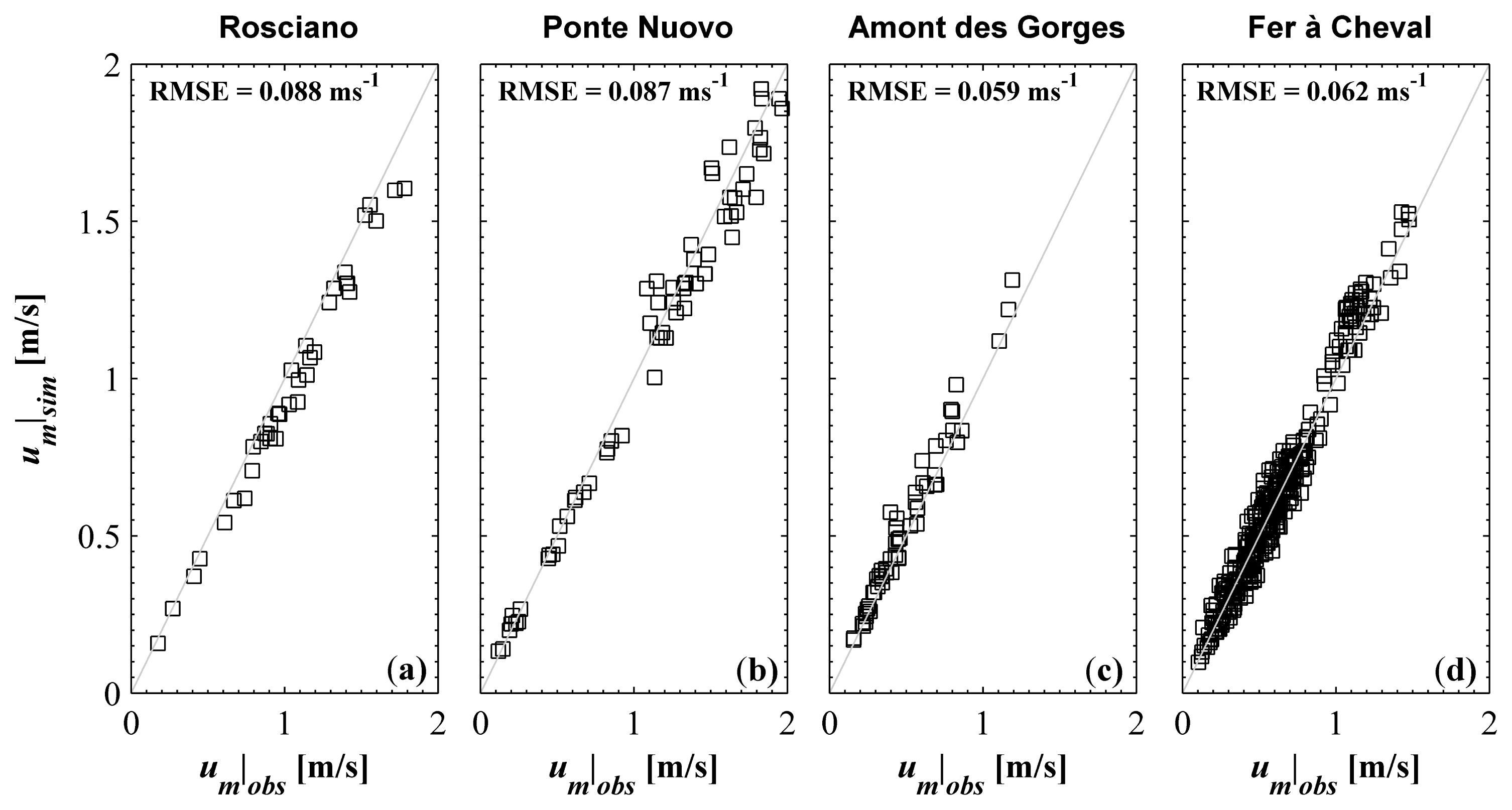
Table 3) using actual velocity data. Therefore, on the basis of the Φ values thus estimated and using
Equation (6), the mean flow velocities,
um, are estimated and compared with the observed values. The comparison is illustrated in
Figure 5 in which the root mean square error, RMSE, is also shown. A generally good match between the observed and computed velocities is found with a slight underestimation at the Rosciano river site, possibly due to a change in the river cross section shape between the two periods. However the RMSE of the
um estimation is less than 0.09 m/s for all river sites.
Based on these results, it is evident that if for a gauged river site a historical sample of standard velocity measurements is available for mid-low water levels, but there is no information concerning umax, the sampling of umax would be enough to obtain a reliable estimation of Φ and thus um, for high flow estimates. This finding could be of considerable interest, in particular with the increased use of radar sensors for monitoring water levels and surface velocities, for the monitoring of high flows at sites where it is only possible to sample velocity at the water surface using conventional gauging methods.


