How to Mine Information from Each Instance to Extract an Abbreviated and Credible Logical Rule

Abstract

Decision trees are particularly promising in symbolic representation and reasoning due to their comprehensible nature, which resembles the hierarchical process of human decision making. However, their drawbacks, caused by the single-tree structure, cannot be ignored. A rigid decision path may cause the majority class to overwhelm other class when dealing with imbalanced data sets, and pruning removes not only superfluous nodes, but also subtrees. The proposed learning algorithm, flexible hybrid decision forest (FHDF), mines information implicated in each instance to form logical rules on the basis of a chain rule of local mutual information, then forms different decision tree structures and decision forests later. The most credible decision path from the decision forest can be selected to make a prediction. Furthermore, functional dependencies (FDs), which are extracted from the whole data set based on association rule analysis, perform embedded attribute selection to remove nodes rather than subtrees, thus helping to achieve different levels of knowledge representation and improve model comprehension in the framework of semi-supervised learning. Naive Bayes replaces the leaf nodes at the bottom of the tree hierarchy, where the conditional independence assumption may hold. This technique reduces the potential for overfitting and overtraining and improves the prediction quality and generalization. Experimental results on UCI data sets demonstrate the efficacy of the proposed approach.

1. Introduction

The rapid development of information and web technology has made a significant amount of data readily available for knowledge discovery. Growing interest in symbolic representation and reasoning highlights knowledge discovery as a clearly identifiable and technically rich subfield in artificial intelligence. The desirable properties of tools used to investigate big data are easy to understand models and predictive decisions. Decision trees are particularly promising in this regard, due to their comprehensible nature that resembles the hierarchical process of human decision making. To split nodes while growing the tree, the vast majority of the oblique and univariate decision-tree induction algorithms employ different impurity-based measures [1,2]. Aside from such advantages, such as the ability to explain the decision process and low computational costs, their drawbacks, caused by the single-tree structure, cannot be ignored.

Commonly, to classify an instance, we can just follow one path from the unique root to the leaf, examining every decision made along the way. This approach usually works well. However, in reality, the classification distribution is frequently used to deal with imbalanced datasets, where there are many more instances of a certain class than of another. In such cases, a rigid decision path may cause the majority class overwhelm other classes, thus creating a situation where the minority class is ignored. The decision tree corresponds to locally optimal solutions to all training data, but from it, we cannot get globally optimal solutions to the whole data set. Besides, low-quality training data may lead to the construction of overfitting or fragile classifiers. Thus, eliminating redundant attributes is generally used as a data preprocessing technique to improve the quality of the data. However, pruning removes not only superfluous nodes, but also subtrees, with the superfluous nodes as subroots. If some key nodes are removed by mistake, the negative effect caused by the absent nodes may propagate and aggravate the situation to some extent. To ensure a credible and robust decision path, according to Occam’s razor rule, only a limited number of attributes can be used for prediction. Thus just a portion of the information implicated in the training data will be utilized.

To resemble the hierarchical process of human decision making and to make the final model much more flexible, the core idea of this paper is to build a decision forest rather than a single tree to model training data. The theoretical foundation of the traditional decision tree algorithm is the chain rule of joint mutual information, which applies mutual and conditional mutual information to describe the direct and indirect relationships between predictive attributes and the class label. Correspondingly, the proposed learning algorithm, flexible hybrid decision forest (FHDF), applies the chain rule of local mutual information to form logical rules for each instance. The rules with the same root form different decision tree structures and then form a decision forest later. Thus, we can choose the most credible path from the forest to classify. To reduce the potential for overfitting and overtraining, functional dependencies (FDs) [3,4] will be employed as prior knowledge to remove redundant attributes rather than subtrees. Additionally, different sets of redundant attributes may be found and removed from different test instances. Because FDs are unrelated to class label, they can be extracted from the whole data set, rather than training data based on association rule analysis [5]; thus, FHDF works in the framework of semi-supervised learning. Naive Bayes (NB) [6,7], which is an important mining classifier for data mining and applied in many real-world classification problems, because of its high classification performance, replaces the leaf nodes at the bottom of the tree hierarchy, where the conditional independence assumption may hold. This technique ensures that all attributes will be utilized for prediction, thus improving the prediction quality and generalization.

The rest of this paper is organized as follows. Section 2 first proposes the theoretical basis of decision forest—the chain rule of local mutual information—then clarifies the rationality of FDs and introduces related work about NB. Section 3 describes the learning procedure of FHDF. Section 4 compares various approaches on data sets from the UCI repository. Finally, Section 5 presents possible future work.

2. Related Research Work

2.1. Information Theory

In the 1940s, Claude E. Shannon introduced information theory, the theoretical basis of modern digital communication. Although Shannon was principally concerned with the problem of electronic communications, the theory has much broader applicability. Many commonly used measures are based on the entropy of information theory and used in a variety of classification algorithms.

In the following discussion, Greek letters (α, β, γ) denote sets of attributes. Lower-case letters denote specific values taken by corresponding attributes (for instance, x_i represents the event that X_i = x_i).

Definition 1

Entropy is a measure of uncertainty of random variable C:

$$H(C)=-\sum _{c\in C}P(c)\hspace{0.17em}\text{log\hspace{0.17em}}P(c)$$

(1)

where P(c) is the marginal probability distribution function of C.

Definition 2

Mutual information I(C; X) is the reduction of entropy about variable C after observing all possible values of X

$$MI(C;X)=H(C)-H(C\mid X)=\sum _{x\in X}\sum _{c\in C}P(x,c)\hspace{0.17em}\text{log\hspace{0.17em}}\frac{P(x,c)}{P(c)P(x)}$$

(2)

where P(x, c) is the joint probability distribution function of X and C.

Definition 3

Local mutual information LMI(C; x) is defined to measure the reduction of entropy about variable C after observing X = x,

$$LMI(C;x)=\sum _{c\in C}P(x,c)\hspace{0.17em}\text{log}\frac{P(x,c)}{P(c)P(x)}$$

(3)

Definition 4

Conditional mutual information CMI(C;X_i|X_j) is defined to measure the expected value of the mutual information of two random variables C and X_i given the value of a third variable X_j.

$$CMI(C;X_i\mid X_j)=\sum _{c\in C}\sum _{x_i\in X_i}\sum _{x_j\in X_j}P(x_i,c\mid x_j)\hspace{0.17em}\text{log\hspace{0.17em}}\frac{P(x_i,c\mid x_j)}{P(c\mid x_j)P(x_i\mid x_j)}$$

(4)

Definition 5

Conditional local mutual information CLMI(C; x_i|x_j) is defined to measure the reduction of entropy about variable C after observing X_i = x_i when X_j = x_j always holds.

$$CLMI(C;x_i\mid x_j)=\sum _{c\in C}P(x_i,c\mid x_j)\hspace{0.17em}\text{log}\frac{P(x_i,c\mid x_j)}{P(c\mid x_j)P(x_i\mid x_j)}$$

(5)

Obviously,

$$\{\begin{array}{l}I(C;X)={\sum }_{X}LMI(C;x)\hfill \\ CMI(C;X_i\mid X_j)={\sum }_{X_i}{\sum }_{X_j}CLMI(C;x_i\mid x_j)\hfill \end{array}$$

(6)

Mutual information and conditional mutual information are commonly applied to roughly describe the direct or conditional relationships between predictive attribute and class label C. However, in the real world, the relationships between attributes may differ greatly as the situation changes. Local mutual information and conditional local mutual information can be used to describe the dynamic changes, thus making the final model much more flexible. For example, as Figure 1 shows, suppose that the overall relationship among attributes {X₂, · · ·, X₃} and class label C is just like a rectangle. However, for the k–th instance, {X₂,X₃} are independent of C, and the local relationship between X₁ and C is just like an oval.

According to the chain rule of joint mutual information, which is the theoretical basis of the decision tree learning algorithm, the mutual information between attributes X = {X₁,X₂, · · ·, X_n} and class label C is:

$$MI(C;X)=MI(C;X_1)+CMI(C;X_2\mid X_1)+\cdots +CMI(C;X_n\mid X_1,\cdots ,X_{n-1})$$

(7)

On the other hand, for a sample t = {x₁, x₂, · · ·, x_n} in data set S, the chain rule of local mutual information between t and class label C can be represented as:

$$LMI(C;t)=LMI(C;x_1)+CLMI(C;x_2\mid x_1)+\cdots +CLMI(C;x_n\mid x_1,\cdots ,x_{n-1})$$

(8)

On the basis of the chain rule of local mutual information described above, we can convert each instance into a single logical rule or decision path. We first choose the most appropriate attribute value from t, e.g., x₁, which satisfies LMI(C; x₁) = max LMI(C; x_i)(1 ≤ i ≤ n). The training set is split into finer subsets with attribute value x₁. Then, we choose the next attribute value, e.g., x₂, which satisfies CLMI(C; x₂|x₁) = max CLMI(C; x_i|x₁)(1 ≤ i ≤ n, i ≠ 1). The training subset is further split into finer subsets with attribute values x₁ and x₂. This procedure will continue, until the class label of the subset is the same or the instances in the subset satisfy some criterion. Finally, each training instance corresponds to a logical rule or decision path. If several rules have the same root, the combination of these rules with the same root node can build a complete decision tree, and the same part of the structural information present in the data can be expressed. Thus, the final model is composed of not one tree, but one forest. This technique reduces the potential for overfitting and overtraining and improves the prediction quality and generalization. For example, given attributes X = {X₁,X₂,X₃,X₄} and three instances {t₁, t₂, t₃}, according to the comparison results of local mutual information and conditional local mutual information instances, {t₁, t₂, t₃} can be converted into three logical rules. The conversion procedure are shown in Figure 2.

Because Rule 2 and Rule 3 have the same root, they can be combined into a single tree. Finally, from instances {t₁, t₂, t₃}, we can build two tree structure, as Figure 3 shows.

2.2. Functional Dependency Rules of Probability

Given a relation R (in a relational database), attribute Y of R is functionally dependent on attribute X of R, and X of R functionally determines Y of R (in symbols X → Y ). We demonstrated functional dependency rules of probability in [8,9] to build a linkage between FD and probability theory, and the following rules are mainly included:

• Representation equivalence of probability: Suppose data set S consists of two attribute sets {α, β} and β can be inferred by α, i.e., the FD α → β holds, then the following joint probability distribution holds:
  $$P(\alpha )=P(\alpha ,\beta )$$

  (9)
• Augmentation rule of probability: If FD α → β holds and γ is a set of attributes, then the following joint probability distribution holds:
  $$P(\alpha ,\gamma )=P(\alpha ,\beta ,\gamma )$$

  (10)
• Transitivity rule of probability: If FDs α → β and β → γ hold, then the following joint probability distribution holds:
  $$P(\alpha )=P(\alpha ,\gamma )$$

  (11)
• Pseudo-transitivity rule of probability: If βγ → δ and α → β hold, then the joint probability distribution holds:
  $$P(\alpha ,\gamma )=P(\alpha ,\gamma ,\delta )$$

  (12)

When two attributes are strongly related, the classifier may overweight the inference from the two attributes, resulting in prediction bias. FDs will help to avoid this situation, and the high dimensional representation or even whole classification model is simplified. For example, if FD x₁ → x₂ exists, for instance t = {x₁, x₂, · · ·, x_n}, by applying the representation equivalence of probability and the augmentation rule of probability, we will have:

$$\{\begin{array}{l}P(x)=P(x_1,x_3,\cdots ,x_n)\hfill \\ P(x,c)=P(x_1,x_3,\cdots ,x_n,c)\hfill \end{array}$$

(13)

Then, from the definition of LMI, we will get:

$$\begin{array}{l}LMI(C\mid x)=\sum _{c\in C}P(x,c)\hspace{0.17em}\text{log\hspace{0.17em}}\frac{P(x,c)}{P(c)P(x)}\\ =\sum _{c\in C}P(x_1,x_3,\cdots ,x_n,c)\hspace{0.17em}\text{log\hspace{0.17em}}\frac{P(x_1,x_3,\cdots ,x_n,c)}{P(c)P(x_1,x_3,\cdots ,x_n)}=LMI(C\mid x_1,x_3,\cdots ,x_n)\end{array}$$

(14)

Thus, x₂ is extraneous to classify t. Obviously, extraneous attributes reduction resulting from FDs will not change underlying conditional probability, thus, in turn, leading to lower variance. Therefore, FDs have the potential to be a valuable supplementary of the classifier over a considerable range of classification tasks. Discovering FDs from existing databases is an important issue, investigated for many years, and recently addressed with a data mining viewpoint, in a novel and much more efficient way [10,11].

2.3. Naive Bayes

Supervised classification is a basic task in artificial intelligence and knowledge discovery. The aim of supervised learning is to predict from a training set the class of a testing instance x = {x₁, · · ·, x_n}, where x_i is the value of the i-th attribute. We estimate the conditional probability of P(c|x) by selecting arg max_C P(c|x), where c ∈ {c₁, · · ·, c_k} are the k classes. From Bayes theorem, we have:

$$P(c\mid x)=P(c,x)/P(x)\propto P(c,x)\propto P(x\mid c)P(c)$$

(15)

The BN classifier is becoming increasingly popular in many areas, such as decision aid, diagnosis and complex system control, because of its inference capabilities [12,13]. The structure of BN is a directed acyclic graph, where the nodes correspond to domain attributes and the arcs between the nodes represent direct dependencies between the attributes. The absence of an arc between two nodes X₁ and X₂ denotes that X₂ is independent of X₁ given its parents.

However, the accurate estimation of P(x|c) is a complex process. Learning an optimal BN structure from existing data has been proven to be an NP-hard problem. NB avoids this problem by assuming that the attributes are independent given the class,

$$P(x\mid c)=\prod _{i=1}^{n}P(x_i\mid c).$$

(16)

Then, the following equation is often calculated in practice rather than Equation (15).

$$P(c\mid x)\propto P(c)\prod _{i=1}^{n}P(x_i\mid c)$$

(17)

NB has a simple structure, whereby an arc exists from the class node to other nodes, but no arcs exist among the other nodes, as illustrated in Figure 4. One advantage of NB is avoiding model selection, because selecting between alternative models can be expected to increase variance and allow a learning system to over fit the training data [14].

3. FHDF

The learning procedure of the FHDF algorithm is described as follows:

• Input: Training set T₁, testing set T₂, predictive attribute set X = {X₁, · · ·, X_n} and class label C.
• Output: Hybrid decision forest model.
• Pre-processing phase: Mine association rules from data set T₁ + T₂, then convert them into FDs; achieve the closure of FDs. Find extraneous attributes based on FD analysis and remove them from attribute set.

Training phase:

Step 1

For each instance t = {x₁, · · ·, x_n} in T₁, generate the root node X_i that satisfies

$$X_i=\text{arg\hspace{0.17em}max\hspace{0.17em}}LMI(C;x_p)(1\le p\le n)$$

Then, verify if the corresponding subset, which satisfies X_i = x_i, has the same class label.

(a)

If yes, exit and create a leaf node;

(b)

Otherwise, node X_i is created and added as one branch node.

Step 2

Calculate for each attribute value, among the attributes that have not been used so far, its CLMI and select attribute X_j, which satisfies:

$$X_j=\text{arg\hspace{0.17em}max\hspace{0.17em}}CLMI(C;x_q\mid x_i)(1\le q\le n,q\ne i)$$

Then, verify if CLMI satisfies the stopping criterion: (a) If yes, create NB as a leaf node; (b) otherwise, child node X_j is created and added to the branch. Repeat the same process for each instance t in T₁ from Step 1.

Step 3

Get the order of attribute values in each instance, which will be converted into the classification rule. Use the rules with the same root to construct a hybrid decision tree.

Testing phase:

Step 4

Use the rules to assign class labels to unlabeled instances in T₂.

Step 5

For any instance t that does not match any rule in the decision forest, start from the training phase, achieve the attribute order and get the sub-optimal rule for classification.

Knowledge implicated in a database can be divided into certain and uncertain parts. The certain part is commonly described by a set of rules, such as a decision tree. The uncertain part is always described from the viewpoint of probability, such as BN. The proposed working mechanism of the hybrid model-FHDF resembles the hierarchical process of human decision making. First, we convert each instance into a rule form by applying the chain rule of local mutual information. The extracted robust knowledge structure can solve the most certain problems based on definite knowledge and experience. Second, if the criterion of information growth cannot be satisfied, that means knowledge is scattered, and the independence assumption may be satisfied to some extent; then, NB is applied to make full use of the rest of the attributes.

Before this structured learning process of knowledge accumulation and induction, FDs is utilized to remove extraneous information to build a simplified and robust knowledge structure. For example, suppose data set S, and the logical rules inferred are shown in

Table 1. Corresponding classification rules.

No	Rules	Class Label
1	{a0} →	C1
2	{a0} →	C1
3	{a1, b0, c0} →	C2
4	{a1, b0, c1} →	C1
5	{a1, b0, c2} →	C2
6	{a2, b1} →	C0
7	{a2, b0} →	C1
8	{b2} →	C2
9	{b2} →	C2
⋮	⋮	⋮

and

Table 2. Sample data from data set S.

No	X1	X2	X3	Class Label
1	a0	b0	c2	C1
2	a0	b1	c1	C1
3	a1	b0	c0	C2
4	a1	b0	c1	C1
5	a1	b0	c2	C2
6	a2	b1	c1	C0
7	a2	b0	c1	C1
8	a3	b2	c0	C2
9	a4	b2	c1	C2
⋮	⋮	⋮	⋮	⋮

, respectively; the corresponding FHDF structure will be as Figure 5a shows. If FD {X₁ = a₁} → {X₂ = b₀} holds, for instance three, four and five X₂ are extraneous for further inference. As Figure 5b shows, X₂ will be removed from the FHDF structure.

Equation (8) is the theoretical basis of FHDF. For each instance t in the training set, According to Occam’s razor rule, a shorter assumption may be believable, but a longer one is highly coincidental. To make the final prediction credible, information growth must be assured when attributes are added in order. When adding new attribute x_i, the stopping prerequisite should be as follows:

$$LMI(C;x_1,\cdots ,x_i)>1.2\times LMI(C;x_1,\cdots ,x_{i-1})$$

The information growth must be more than 20%. Otherwise, FHDF creates an NB leaf node with all of the other attributes that have not been processed to perform further inference.

To sum up, FHDF extracts logical rules from the logical viewpoint by calculating LMI and CLMI, while NB predicts from the probabilistic viewpoint. Besides, FHDF presents outstanding flexibility and adaptability when there is a lack of prior knowledge. For example, given a testing instance t = {a₃, b₁, c₀}, no rule in the decision forest can be used to assign a class label. Suppose that the attribute order is {c₀, a₃, b₁} by calculating LMI and CLMI; as shown in Table 1, only training Instance 8 meets the first two conditions and can be used to classify t. The class label of t should be C₂.

4. Experiments

4.1. Bias and Variance

Kohavi and Wolpert presented a bias-variance decomposition of expected misclassification rate [15], which is a powerful tool from sampling theory statistics for analyzing supervised learning scenarios. Suppose c and ĉ are the true class label and that generated by a learning algorithm, respectively, the zero-one loss function is defined as:

$$\xi (c,\widehat{c})=1-\delta (c,\widehat{c}),$$

where δ(c, ĉ) = 1 if ĉ = c and zero otherwise. The bias term measures the squared difference between the average output of the target and the algorithm. This term is defined as follows:

$$bias=\frac{1}{2}\sum _{\widehat{c},c\varepsilon C}{[P(\widehat{c}\mid x)-P(c\mid x)]}^2,$$

where x is the combination of any attribute value. The variance term is a real valued non-negative quantity and equals zero for an algorithm that always makes the same guess regardless of the training set. The variance increases as the algorithm becomes more sensitive to changes in the training set. It is defined as follows:

$$variance=\frac{1}{2}[1-\sum _{\widehat{c}\varepsilon C}P{(\widehat{c}\mid x)}^2].$$

Moore and McCabe illustrated bias and variance through shooting arrows at a target [16], as described in Figure 6. The perfect model can be regarded as the bull’s eye on a target and the learned classifier as an arrow fired at the bull’s eye. Bias and variance describe what happens when an archer fires many arrows at the target. Bias means that the aim is off and the arrows land consistently off the bull’s eye in the same direction. Variance means that the arrows are scattered. Large variance means that repeated shots are widely scattered on the target. They do not give similar results, but differ widely among themselves.

4.2. Statistical Results on UCI Data Sets

In order to verify the efficiency and effectiveness of the proposed FHDF, we conduct experiments on 43 data sets from the UCI machine learning repository.

Table 3. Data sets.

No.	Data Set	# Instance	Attribute	Class
1	Abalone *	4177	9	3
2	Adult *	48,842	15	2
3	Anneal	898	39	6
4	Audio	226	70	24
5	Balance Scale (Wisconsin)	625	5	3
6	breast-cancer-w	699	10	2
7	Live Disorder (Bupa)	345	7	2
8	Car	1728	8	4
9	Chess	551	40	2
10	Cleveland	303	14	2
11	Connect-4 Opening *	67,557	43	3
12	Contraceptive Method Choice	1473	10	3
13	Credit Screening	690	16	2
14	Cylinder-bands	540	40	2
15	Dermatology	366	35	6
16	Glass Identification	214	10	3
17	German	1000	21	2
18	Haberman’s Survival	306	4	2
19	Heart Disease	303	14	2
20	Hepatitis	155	20	2
21	Hungarian	294	14	2
22	Iris	150	5	3
23	King-rook-vs-King-pawn *	3196	36	2
24	Labor Negotiation	57	17	2
25	LED	1,000	8	10
26	Localization *	164,860	7	3
27	Lung Cancer	32	57	3
28	Lymphography	148	19	4
29	Magic *	19,020	11	2
30	Mushroom *	8124	22	2
31	Nursery *	12,960	8	5
32	Optdigits *	5620	64	10
33	Poker-hand	1,025,010 *	11	10
34	Primary Tumor	339	18	22
35	Satellite *	6435	37	6
36	Segment *	2310	20	7
37	Shuttle *	58,000	9	7
38	Sick *	3772	30	2
39	Spambase *	4601	58	2
40	Teaching Assistant Evaluation	151	6	3
41	Vehicle	846	19	4
42	Wine Recognition	178	14	3
43	Zoo	101	17	7

summarizes the characteristics of each data set, including the number of instances, attributes and classes. Large data sets with an instance number greater than 3000 are annotated with the symbol “*”. Missing values for qualitative attributes are replaced with modes, and those for quantitative attributes are replaced with means from the training data. For each benchmark data set, numeric attributes are discretized using MDL discretization [17]. The following techniques are compared:

• NB, standard naive Bayes.
• TAN [18], tree-augmented naive Bayes applying incremental learning.
• C4.5, standard decision tree.
• NBTree [19], decision tree with naive Bayes as the leaf node.
• RTAN [20], tree-augmented naive Bayes ensembles.

All algorithms were coded in MATLAB 7.0 on a Pentium 2.93 GHz/1 G RAM computer.

Base probability estimates P(c), P(c, x_i) and P(c, x_i, x_j) were smoothed using the Laplace estimate, which can be described as follows:

$$\{\begin{array}{l}\widehat{P}(c)=\frac{F(c)+1}{K+k}\hfill \\ \widehat{P}(c,x_i)=\frac{F(c,x_i)+1}{K_i+k_i}\hfill \\ \widehat{P}(c,x_i,x_j)=\frac{F(c,x_i,x_j)+1}{K_{ij}+k_{ij}}\hfill \end{array}$$

(18)

where F(·) is the frequency with which a combination of terms appears in the training data, K is the number of training instances for which the class value is known, K_i is the number of training instances for which both the class and attribute X_i are known and K_ij is the number of training instances for which all of the class and attributes X_i and X_j are known. k is the number of attribute values of class C, k_i is the number of attribute value combinations of C and X_i and k_ij is the number of attribute value combinations of C, X_j and X_i.

Semi-supervised learning falls between unsupervised learning (without any labeled training data) and supervised learning (with completely labeled training data). Semi-supervised learning is a class of machine learning techniques that uses both labeled and unlabeled data for training. Typically, a small amount of labeled data with a large amount of unlabeled data is used. Many machine learning researchers have found that when unlabeled data are used in conjunction with a small amount of labeled data, a considerable improvement in learning accuracy can be achieved. The acquisition of labeled data for a learning problem often requires a skilled human agent (e.g., to transcribe an audio segment) or a physical experiment (e.g., determining the 3D structure of a protein or determining whether oil is present at a particular location). Given data set S with attribute set X, suppose FD α → β has been deduced from whole data set and α, β ⊂ X. From the representation equivalence of probability, we can obtain:

$$P(\alpha )=P(\alpha ,\beta )$$

(19)

By applying the augmentation rule of probability, we will get:

$$P(\alpha ,c)=P(\alpha ,\beta ,c)\hspace{0.17em}or\hspace{0.17em}P(\alpha \mid c)=P(\alpha ,\beta \mid c)$$

(20)

Therefore, FD α → β still holds in the training data regardless of the class label. Thus, we can use the whole data set to extract FDs with high confidence. Additionally, the framework of FHDF is semi-supervised learning. In the following discussion, we use FDs that are extracted based on the association rule analysis as the domain knowledge. These rules can be effective in uncovering unknown relationships, thereby providing results that can be the basis of forecast and decision. They have proven to be useful tools for an enterprise, as they strive to improve their competitiveness and profitability. To ensure the validity of FDs, the minimum number of instances that satisfies FD is 100. With the increasing number of attributes, more RAM is needed to store joint probability distributions. An important restriction of our algorithm is that the number of the left side of FD, i.e., the number of key attributes, should be no more than two.

Table 4. Experimental results of 0–1 loss. C4.5, standard decision tree; TAN, tree-augmented naive Bayes applying incremental learning; NBTree, decision tree with naive Bayes as the leaf node; RTAN, tree-augmented naive Bayes ensembles.

Dataset	C4.5	NB	TAN	NBTree	RTAN	FHDF
Abalone	0.460	0.472	0.459	0.430	0.450	0.443
Adult	0.139	0.158	0.138	0.143	0.144	0.131
Anneal	0.458	0.375	0.375	0.360	0.173	0.238
Audio	0.314	0.239	0.292	0.195	0.235	0.307
Balance Scale (Wisconsin)	0.306	0.285	0.280	0.286	0.297	0.278
breast-cancer-w	0.056	0.026	0.042	0.034	0.032	0.071
Live Disorder(Bupa)	0.444	0.444	0.444	0.426	0.452	0.421
Car	0.156	0.140	0.057	0.078	0.061	0.036
Chess	0.151	0.113	0.093	0.096	0.109	0.095
Cleveland	0.277	0.162	0.205	0.171	0.178	0.204
Connect-4 Opening	0.206	0.278	0.235	0.232	0.233	0.217
Contraceptive Method Choice	0.493	0.504	0.489	0.474	0.505	0.475
Credit Screening	0.133	0.141	0.151	0.134	0.142	0.139
Cylinder-bands	0.307	0.215	0.283	0.181	0.179	0.215
Dermatology	0.079	0.019	0.033	0.016	0.022	0.062
Glass Identification	0.257	0.262	0.220	0.242	0.210	0.168
German	0.277	0.253	0.273	0.238	0.259	0.275
Haberman’s Survival	0.281	0.281	0.281	0.270	0.287	0.267
Heart Disease	0.237	0.178	0.193	0.164	0.195	0.201
Hepatitis	0.161	0.194	0.168	0.173	0.184	0.178
Hungarian	0.194	0.160	0.170	0.160	0.163	0.171
Iris	0.080	0.087	0.080	0.083	0.088	0.082
King-rook-vs-King-pawn	0.022	0.121	0.078	0.081	0.068	0.040
Labor Negotiation	0.088	0.035	0.053	0.050	0.036	0.033
LED	0.309	0.267	0.266	0.257	0.271	0.249
Localization	0.305	0.496	0.358	0.345	0.277	0.282
Lung Cancer	0.625	0.438	0.594	0.480	0.510	0.534
Lymphography	0.284	0.149	0.176	0.162	0.152	0.225
Magic	0.164	0.224	0.168	0.168	0.166	0.156
Mushroom	0.000	0.020	0.000	0.000	0.000	0.000
Nursery	0.050	0.097	0.065	0.070	0.053	0.027
Optdigits	0.230	0.077	0.041	0.030	0.024	0.035
Poker-hand	0.245	0.499	0.330	0.462	0.121	0.186
Primary Tumor	0.584	0.546	0.543	0.552	0.557	0.544
Satellite	0.154	0.181	0.121	0.110	0.094	0.103
Segment	0.092	0.079	0.039	0.033	0.034	0.045
Shuttle	0.001	0.004	0.002	0.001	0.001	0.001
Sick	0.020	0.031	0.026	0.026	0.025	0.021
Spambase	0.083	0.102	0.067	0.065	0.058	0.060
Teaching Assistant Evaluation	0.596	0.497	0.550	0.470	0.493	0.360
Vehicle	0.331	0.392	0.294	0.278	0.278	0.280
Wine Recognition	0.107	0.017	0.034	0.022	0.023	0.018
Zoo	0.198	0.030	0.010	0.029	0.010	0.047

presents for each data set the zero-one loss, which is estimated by 10-fold cross-validation to give an accurate estimation of the average performance of an algorithm. The bias and variance results are shown in

Table 5. Experimental results of bias.

Dataset	NB	TAN	C4.5	NBTree	RTAN	FHDF
Abalone	0.404	0.320	0.311	0.333	0.314	0.329
Adult	0.140	0.108	0.100	0.113	0.113	0.108
Connect-4 Opening	0.233	0.183	0.200	0.192	0.209	0.179
King-rook-vs-King-pawn	0.111	0.067	0.019	0.070	0.062	0.039
Localization	0.382	0.326	0.309	0.321	0.314	0.314
Magic	0.199	0.136	0.139	0.161	0.154	0.132
Mushroom	0.040	0.000	0.003	0.001	0.000	0.001
Nursery	0.073	0.051	0.083	0.052	0.042	0.042
Optdigits	0.066	0.031	0.109	0.030	0.022	0.029
Poker-hand	0.327	0.227	0.308	0.263	0.270	0.331
Satellite	0.166	0.094	0.101	0.080	0.075	0.081
Segment	0.086	0.045	0.072	0.039	0.039	0.039
Shuttle	0.007	0.002	0.003	0.002	0.002	0.003
Sick	0.023	0.023	0.022	0.024	0.023	0.021
Spambase	0.097	0.066	0.072	0.067	0.063	0.050

and

Table 6. Experimental results of variance.

Dataset	NB	TAN	C4.5	NBTree	RTAN	FHDF
Abalone	0.093	0.161	0.168	0.122	0.174	0.137
Adult	0.027	0.066	0.045	0.059	0.045	0.044
Connect-4 Opening	0.095	0.088	0.126	0.084	0.083	0.110
King-rook-vs-King-pawn	0.025	0.019	0.010	0.008	0.022	0.023
Localization	0.191	0.256	0.190	0.217	0.232	0.219
Magic	0.041	0.079	0.085	0.065	0.070	0.061
Mushroom	0.008	0.001	0.004	0.000	0.000	0.000
Nursery	0.027	0.038	0.024	0.036	0.034	0.030
Optdigits	0.025	0.028	0.172	0.026	0.021	0.024
Poker-hand	0.209	0.231	0.212	0.263	0.232	0.214
Satellite	0.021	0.041	0.089	0.042	0.042	0.049
Segment	0.017	0.021	0.052	0.021	0.015	0.018
Shuttle	0.004	0.001	0.002	0.002	0.001	0.002
Sick	0.006	0.007	0.002	0.004	0.004	0.005
Spambase	0.010	0.017	0.043	0.019	0.013	0.014

, respectively, in which only 15 large data sets are selected, because of statistical significance. The zero-one loss, bias or variance across multiple data sets provides a gross measure of relative performance. Statistically, a win/draw/loss record (W/D/L) is calculated for each pair of competitors A and B with regard to a performance measure M. The record represents the number of data sets in which A respectively beats, loses to or ties with B on M. Small improvements in leave-one-out error may be attributable to chance. Consequently, it may be beneficial to use a statistical test to assess whether an improvement is significant. A standard binomial sign test, assuming that wins and losses are equiprobable, is applied to these records. A difference is considered significant when the outcome of a two-tailed binomial sign test is less than 0.05.

Table 7. Win/draw/loss record (W/D/L) comparison results of 0–1 loss on all data sets.

W/D/L	C4.5	NB	TAN	NBTree	RTAN
NB	22/5/16
TAN	24/10/9	21/8/14
NBTree	28/7/8	28/9/6	19/19/5
RTAN	27/9/7	20/17/6	24/14/5	16/13/14
FHDF	29/9/5	24/9/10	22/15/6	17/12/14	18/11/14

Table 8. W/D/L comparison results of 0–1 loss on large data sets.

W/D/L	C4.5	NB	TAN	NBTree	RTAN
NB	2/1/12
TAN	4/3/8	14/1/0
NBTree	7/2/6	15/0/0	5/8/2
RTAN	7/2/6	11/1/3	8/4/3	6/5/4
FHDF	10/2/3	15/0/0	12/2/1	11/1/3	8/3/4

Table 9. W/D/L comparison results of bias on large data sets.

W/D/L	NB	TAN	C4.5	NBTree	RTAN
TAN	14/1/0
C4.5	12/1/2	3/3/9
NBTree	14/1/0	2/9/4	8/2/5
RTAN	14/1/0	6/6/3	8/3/4	8/6/1
FHDF	14/1/0	7/5/3	9/2/4	7/5/3	5/5/5

–

Table 10. W/D/L comparison results of variance on large data sets.

W/D/L	NB	TAN	C4.5	NBTree	RTAN
TAN	4/0/11
C4.5	5/2/8	6/1/8
NBTree	5/1/9	10/2/3	9/0/6
RTAN	7/0/8	10/2/3	8/2/5	7/3/5
FHDF	4/3/8	11/0/4	8/2/5	7/2/6	6/2/7

show the W/D/L records corresponding to zero-one loss, bias and variance, respectively.

To clarify the main reason why the same classifier performs differently when data size changes, in the following discussion, we propose a new parameter, named clear winning percentage (CWP), which is defined as follows, to evaluate the extent to which one classifier is relatively superior to another.

$$CWP=\frac{Win-Loss}{Win+Draw+Loss}$$

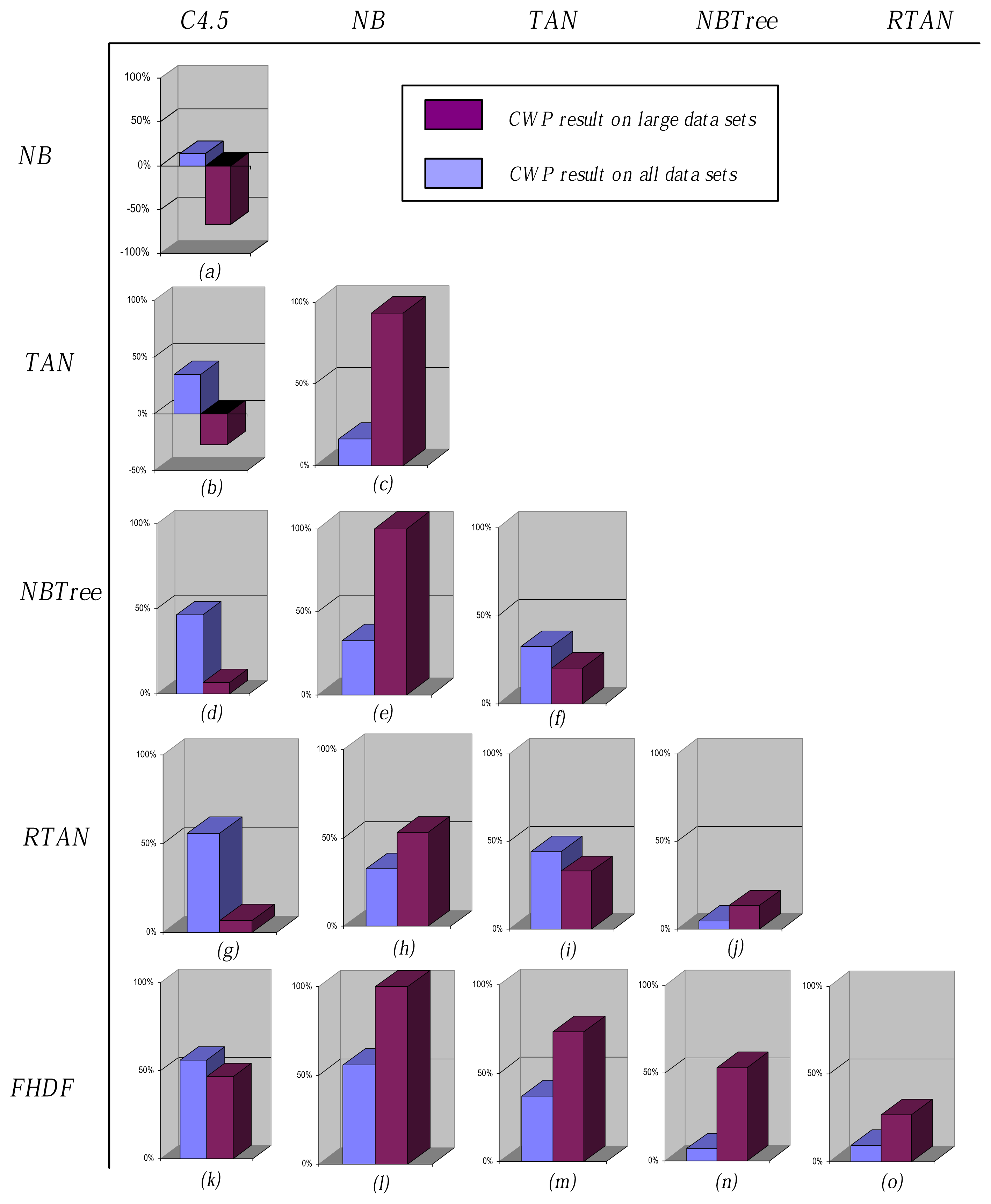
If CWP > 0, then the classifier performs better. Otherwise, it performs worse. Figure 7 shows the comparison results of CWP corresponding to Tables 7 and 8.

NB delivers fast and effective classification with a clear theoretical foundation. However, NB is confronted with the limitations of the conditional independence assumption. From Figure 7a, we can see that, although the conditional independence assumption rarely holds in the real world, NB exhibits competitive performance compared to C4.5, CWP = (22 – 16)/43 = 0.14 > 0. When dealing with small data sets, the instances can be regarded as sparsely distributed, and the conditional independence assumption is satisfied to some extent. For example, there are as many as 38 attributes and only 894 instances for data set “Anneal”. After calculating and comparing the sum of CMI between one attribute and all of the other attributes, most attributes have weak relationships to other attributes or are even nearly independent of them. However, when dealing with large data sets, the relationships between attributes become much more obvious, and the limitation of this assumption cannot be neglected, CWP = (2–12)/15 = −0.67 < 0. As Figure 7b shows, similar result appears when TAN and C4.5 are compared. The main reason may be that logical rules, which are extracted based on information theory, take the main role for classification and can represent credible linear dependency among attributes as data size increases. Besides, as Figure 7c shows, although TAN is restricted to have at most one parent node for each predictive attribute, its structure is more reasonable than NB and can exhibit the relationship between attributes to some extent. From Figure 7d–f, when compared with these three single-structure models, the hybrid model, i.e., NBTree, shows superior or at least equivalent performance. To decrease the computational overhead, NB and TAN simplify the network structure given different independence assumption; whereas the hybrid model can utilize the advantages of both logical rule and probabilistic estimation. Because the leaf of the tree structure contains only limited number instances, NB can evenly make use of the rest of the attributes. RTAN investigates the diversity of TAN by the K statistic. From Figure 7g–j, this bagging mechanism helps RTAN to achieve superior performance to NB and TAN. However, when compared to decision tree learning algorithms, i.e., C4.5 and NBTree, the advantage of RTAN is not obvious. FHDF is motivated by the desire to weaken the assumption by removing correlated attributes on the basis of FD analysis. It also applies the bagging mechanism to describe the hyperplane in which each instance exist. From Figure 7k–o, FHDF demonstrates comprehensive and superior performance.

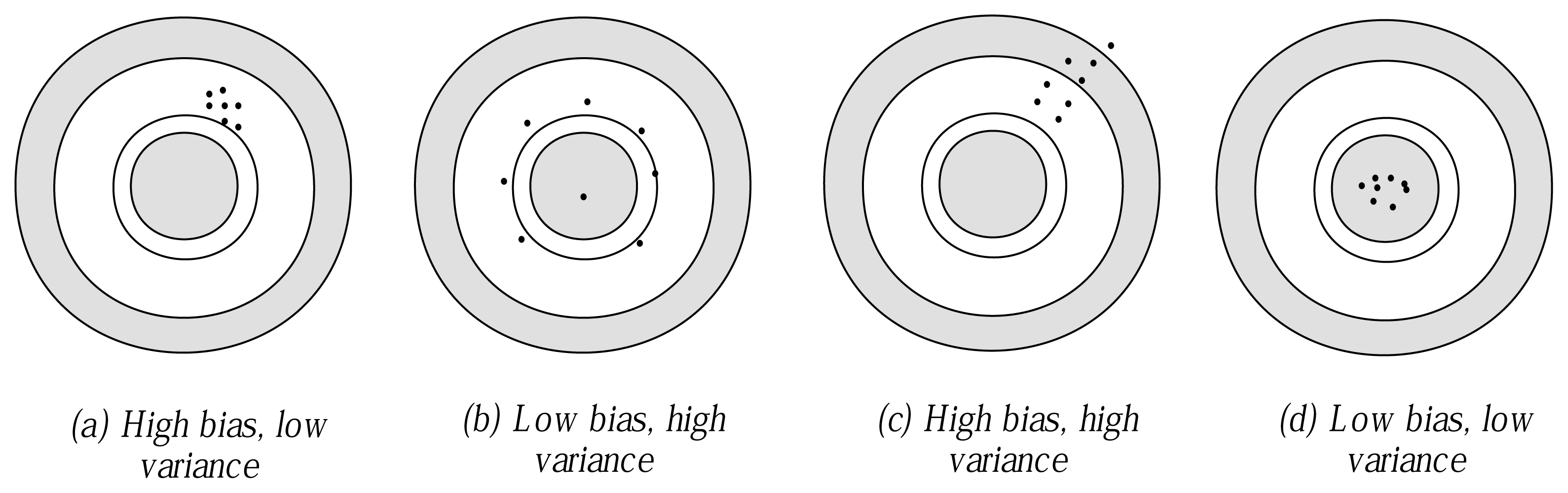
Bias can help to evaluate the extent to which the final model learned from training data fits the whole data set. From Table 9, we can see that the fitness of NB is the poorest, because its structure is definite regardless of what the true data distribution is. In contrast, TAN performs much better than C4.5 and NBTree. The main reason may be that each predictive attribute of TAN is affected by its direct parent node, which is selected by calculating CMI from the global viewpoint. As for C4.5 and NBTree, the final prediction greatly relies on the first few attributes corresponding to the main parts of the singletree structure, i.e., the root and the branch nodes. Thus, C4.5 and NBTree can easily achieve local rather than global optimization solution. Additionally, in view of this, the bagging mechanism can help RTAN and FHDF to make full use of the information that training data supply, since the knowledge hierarchy implicated in the training data can be described in different submodels, and the negative effect caused by data distribution change will be mitigated to a certain extent. The complicated relationship among attributes are measured and depicted from the viewpoint of information theory; thus, performance robustness can be achieved.

With respect to variance, as Table 10 shows, of these algorithms, NB performs the best, because its network structure is definite and, thus, not sensitive to changes in the training set. By contrast, C4.5 performs the worst. The main reason may be that the logical rules resemble the hierarchical process of human decision making. The attributes that locate at the back must correlate with those in the front. If any attribute changes the location, the following attributes will be affected greatly. Thus, for different training sets, especially when the branch contains a very small number of instances, the conditional distribution estimates may differ greatly and different attribute orders may be obtained. For example, there are 58 attributes and 4601 instances for data set “Spambase”. When 10-fold cross-validation is applied, only 4601×0.9 = 4141 instances can be used for training. Suppose each attribute contains two values and the leaf node must have at least 100 instances to ensure statistical significance: each logical rule will use at most five attributes for prediction. That means that the order of the rest of the 53 attributes may be at random. TAN and RTAN need to calculate CMI to build a maximal spanning tree, which may cause overfitting. On the other hand, FHDF and NBTree both use NB as the leaf node, thus retaining the simplicity and direct theoretical foundation of the decision tree, while mitigating the negative effect of the probability distribution of the training set. Besides, when different training and testing sets were given, FHDF uses the same FDs in the semi-supervised learning framework to eliminate redundant attributes. These FDs are extracted from the whole data set and entirely unrelated to the training set.

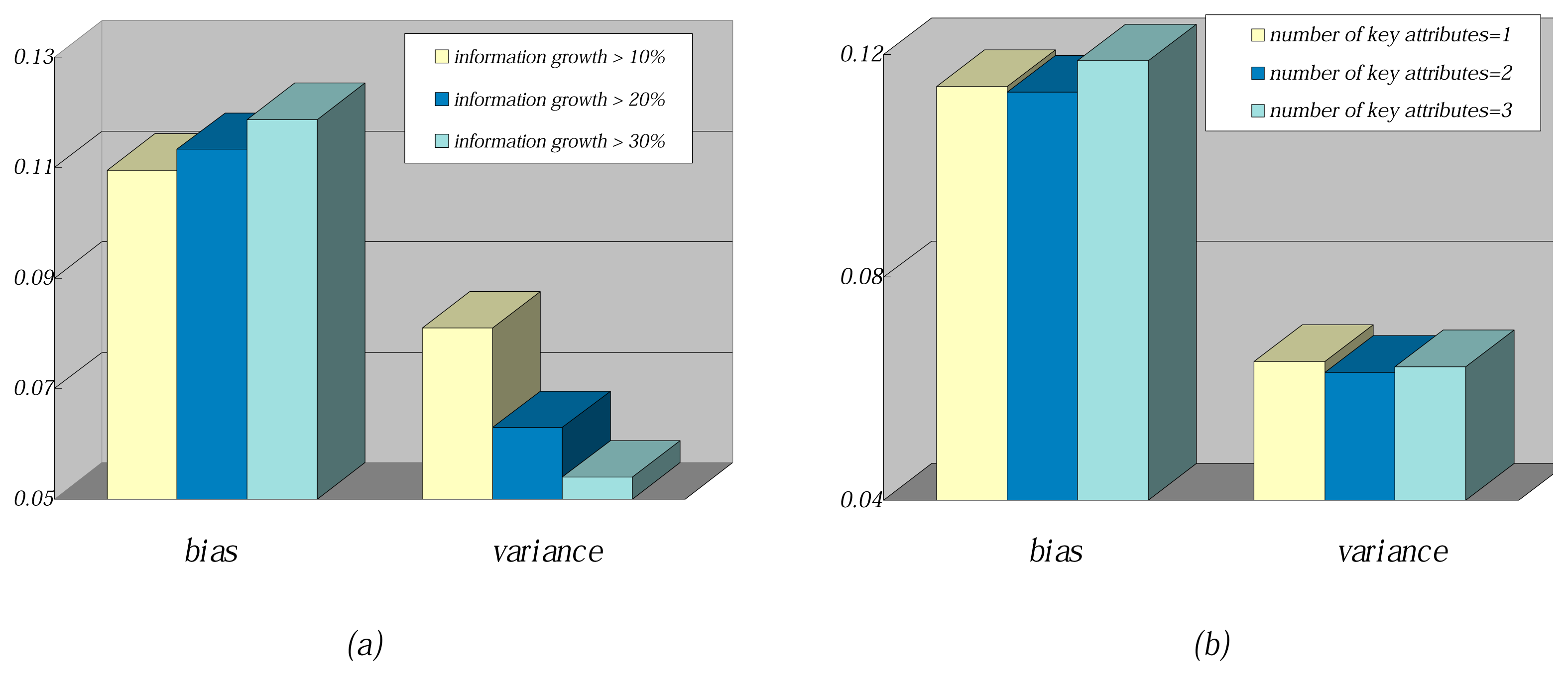
To further describe the working mechanism of FHDF, the information growth and the number of key attributes are changed while learning from training data. The comparison results of average bias and average variance are shown in Figure 8. When information growth increased from 10% to 30%, as can be seen from Figure 8a, the bias increased correspondingly, while the variance decreased. The main reason may be that if instance t needs to be converted into the classification rule, higher information growth will cause fewer attribute values to be selected. Thus, the classification rule will be too short to precisely fit instance t. However, when given different training data, the short rule may roughly hold for many instances. When the number of key attributes increased from one to three, as can be seen from Figure 8b, the bias and variance almost remain the same. With more key attributes used, according to Occam’s razor rule, the extracted FDs may be coincidental and not credible. Furthermore, the number of FDs with one key attribute are much more than those with two or three key attributes; the negative effect on bias and variance can be neglected.

5. Conclusions

FHDF has demonstrated a number of advantages over previous decision tree learning algorithms. With sparsely distributed data, ensemble learning has difficulty in predicting with certainty, thus resulting in an error rate increase. Because regardless of which part is considered as the testing part, FDs are extracted from the whole data set and, thus, remain the same. The computational demands for determining the structure became lower, especially if a large number of attributes are available. The size of the conditional probability tables increased exponentially with the number of parents. Sufficient labeled instances are a prerequisite for the precise parameter estimation. However, from the probabilistic analysis perspective, if the size of the data set is too small, the distributions of different attribute values become uneven. Some attributes may be closely distributed, whereas others may be sparsely distributed. As a result, an unreliable probability estimate might be obtained. To get the precise calculation of CLMI and estimation of the conditional probability distribution, determining when NB can be used as the leaf node remains unsolved. A number of techniques have been developed for extending the decision tree to handle numeric data. Hence, extending the current work to the more general FHDF framework is necessary.

References

1. Suresha, M.; Danti, A.; Narasimhamurthy, S.K. Decision trees to multiclass prediction for analysis of arecanut data. Comput. Syst. Sci. Eng 2014, 29, 105–114. [Google Scholar]
2. Abellan, J.; Baker, R.M.; Crossman, R.J.; Masegosa, A.R. Classification with decision trees from a nonparametric predictive inference perspective. Comput. Stat. Data Anal 2014, 71, 789–802. [Google Scholar] [Green Version]
3. Tao, X.P.; Wang, N.; Zhou, Sh.G.; Zhou, A.Y.; Hu, Y.F. Mining Functional Dependency Rule of Relational Database. Proceedings of the 3rd Pacific-Asia Conference on on Knowledge Discovery and Data Mining, Beijing, China, 26–28 April 1999; Zhong, N., Zhou, L.Z., Eds.; Springer: Berlin/Heidelberg, Germany, 1999; pp. 520–524. [Google Scholar]
4. Ronald, S.K.; James, J.L. Discovery of functional and approximate functional dependencies in relational databases. J. Appl. Math. Dec. Sci 2003, 7, 49–59. [Google Scholar]
5. Agrawal, R.; Srikant, R. Fast algorithms for mining association rules in large databases. Proceedings of 20th International Conference on Very Large Data Bases, Santiago de Chile, Chile, 12–15 September 1994; pp. 487–499.
6. Wu, J.; Cai, Z. A naive Bayes probability estimation model based on self-adaptive differential evolution. J. Intell. Inf. Syst 2014, 42, 671–694. [Google Scholar]
7. Zheng, F.; Webb, G.I. Subsumption Resolution: An Efficient and Effective Technique for Semi-Naive Bayesian Learning. Mach. Learn 2012, 87, 1947–1988. [Google Scholar]
8. Wang, L.M.; Yao, G.F. Extracting Logical Rules and Attribute Subset from Confidence Domain. Information-Tokyo 2012, 15, 173–180. [Google Scholar]
9. Wang, L.M.; Yao, G.F. Learning NT Bayesian Classifier Based on Canonical Cover Analysis of Relational Database. Information-Tokyo 2012, 15, 165–172. [Google Scholar]
10. Wang, L.M.; Yao, G.F. Bayesian Network Inference Based on Functional Dependency Mining of Relational Database. Information-Tokyo 2012, 15, 2441–2446. [Google Scholar]
11. Beskales, G.; Ilyas, I.; Golab, L. Sampling from repairs of conditional functional dependency violations. VLDB J 2014, 23, 103–128. [Google Scholar]
12. Nayyar, A.Z.; Webb, G.I. Fast and Effective Single Pass Bayesian Learning. Proceedings of the 17th Pacific-Asia Conference on on Knowledge Discovery and Data Mining, Gold Coast, Australia, 14–17 April 2013; Pei, J., Vincent, S.T., Cao, L.B., Eds.; Springer: Berlin/Heidelberg, Germany, 2013; pp. 149–160. [Google Scholar]
13. Jiang, L.; Li, C.; Wang, S. Cost-sensitive Bayesian network classifiers. Patt. Recogn. Lett 2014, 45, 211–216. [Google Scholar]
14. Langley, P.; Sage, S. Induction of Selective Bayesian Classifiers. Proceedings of the 10th Conference on Uncertainty in Artificial Intelligence, Seattle, WA, 29–31 July 1994.
15. Kohavi, R.; Wolpert, D. Bias Plus Variance Decomposition for Zero-one Loss Functions. Proceedings of the 13th International Conference on Machine Learning, Bari, Italy, 3–6 July 1996.
16. Moore, D.S.; McCabe, G.P. Introduction to the Practice of Statistics, 4th ed; Michelle Julet: San Francisco, CA, USA, 2002. [Google Scholar]
17. Fayyad, U.M.; Irani, K.B. Multi-Interval Discretization of Continuous-Valued Attributes for Classification Learning. Proceedings of the 13th International Joint Conference on Artificial Intelligence, Chambéry, France, 28 August–3 September 1993.
18. Josep, R.A. Incremental Learning of Tree Augmented Naive Bayes Classifiers. Proceedings of the 18th National Conference on Artificial Intelligence and 14th Conference on Innovative Applications of Artificial Intelligence, Edmonton, Alberta, Canada, 28 July–1 August 2002.
19. Farid, D.M.; Zhang, L.; Rahman, C.M. Hybrid decision tree and naive Bayes classifiers for multi-class classification tasks. Expert Syst. Appl 2014, 41, 1937–1946. [Google Scholar]
20. Ma, Sh.; Shi, H.B. Tree-augmented naive Bayes ensembles. Proceedings of the 3rd International Conference on Machine Learning and Cybernetics, Shanghai, China, 26–29 August 2004.
Figure 1. The overall and local relationships among {X1,X2,X3} and C.
Entropy 16 05242f1
Figure 2. The conversion procedure from instances {t1, t2, t3} to logical rules.
Entropy 16 05242f2
Figure 3. The overall decision forest structure corresponding to instances {t1, t2, t3}.
Entropy 16 05242f3
Figure 4. The network structure of naive Bayes.
Entropy 16 05242f4
Figure 5. The corresponding flexible hybrid decision forest (FHDF) structure before and after applying functional dependency (FD).
Entropy 16 05242f5
Figure 6. Bias and variance in shooting arrows at a target.
Entropy 16 05242f6
Figure 7. The 0–1 loss comparison of learning algorithms on all and large data sets.
Entropy 16 05242f7
Figure 8. Comparison results of the bias and variance of FHDF given different information growth and a different number of key attributes.
Entropy 16 05242f8