Nonadiabatic Molecular Dynamics Based on Trajectories

Abstract
: Performing molecular dynamics in electronically excited states requires the inclusion of nonadiabatic effects to properly describe phenomena beyond the Born-Oppenheimer approximation. This article provides a survey of selected nonadiabatic methods based on quantum or classical trajectories. Among these techniques, trajectory surface hopping constitutes an interesting compromise between accuracy and efficiency for the simulation of medium- to large-scale molecular systems. This approach is, however, based on non-rigorous approximations that could compromise, in some cases, the correct description of the nonadiabatic effects under consideration and hamper a systematic improvement of the theory. With the help of an in principle exact description of nonadiabatic dynamics based on Bohmian quantum trajectories, we will investigate the origin of the main approximations in trajectory surface hopping and illustrate some of the limits of this approach by means of a few simple examples.1. Introduction
Traditionally, ab-initio molecular dynamics (AIMD) is described within the so-called Born-Oppenheimer approximation, which assumes that the electronic and nuclear dynamics can be adiabatically separated [1], due to a large difference in mass between nuclei and electrons. Within this approximation, one usually solves the time-independent electronic Schrödinger equation for a given nuclear configuration [2] and then computes the quantum mechanical forces acting on the nuclei from the gradient of the corresponding eigenvalues, which depend parametrically on the nuclear coordinates and form the so-called potential energy surfaces (PES). However, in the description of most photophysical and photochemical processes, the electronic and nuclear dynamics become entangled, and therefore, more accurate nonadiabatic molecular dynamics schemes that go beyond the Born-Oppenheimer (BO) approximation are required. The most commonly used ab initio nonadiabatic molecular dynamics schemes are those based on the mixed quantum/classical propagation of an ensemble of (quasi-) classical trajectories [3–6], which, to some extent, reproduce the quantum dynamics of the nuclei. These mixed quantum/classical methods are especially popular, because they only require that the necessary electronic structure properties be computed on-the-fly, i.e., only at the points in the configuration space visited during the dynamics, therefore making the calculation of the full potential energy surfaces unnecessary. These approaches can be implemented numerically using electronic structure methods, such as Kohn-Sham Density Functional Theory (DFT) [7,8] and its time-dependent version (TDDFT) [9–12] or wavefunction-based approaches, such as Complete Active Space Self-Consistent Field (CASSCF), Multireference Configuration Interaction (MRCI) and Second-Order Approximate Coupled-Cluster (CC2) [13].
Among all nonadiabatic AIMD schemes, Tully’s fewest switches trajectory surface hopping [14,15] (TSH) and its extensions to mixed quantum/classical dynamics [16] are probably the most widely used. In the framework of TSH, the nuclear wave packets on the different PESs are described as a swarm of independent classical trajectories, while the nonadiabatic couplings induce hops of the trajectories from one electronic state to another; the occurrence of a trajectory hop is governed by the evaluation of a hopping probability, which depends on the temporal evolution of state amplitudes (Tully’s coefficients) and on the value of the nonadiabatic couplings.
Alternative schemes have been proposed for the description of the nonadiabatic dynamics of the nuclear degrees of freedom, among which we quote semiclassical approaches [17,18], extended surface hopping [19,20], quantum/classical Liouville approaches [21,22], hydrodynamic nonadiabatic dynamics [23], linearized nonadiabatic dynamics (LAND-map) [24] or correlated electron-ion dynamics methods [25].
Despite the success of the nonadiabatic trajectory-based approaches, there are many quantum mechanical phenomena that cannot be entirely captured within this framework, namely nuclear quantum effects, like wave packets interference [22] and decoherence [26–28] and tunneling. Quantum dynamics methods based on a quantum mechanical representation of both electronic and nuclear degrees of freedom have also become available (see, for example, [29]). However, their high computational cost and the need for a numerical fit of the relevant PESs prior to propagation have limited their application to just a few nuclear degrees of freedom, and therefore, they are not yet suited for the simulation of complex molecular systems.
One possible way to account for quantum nuclear effects within a trajectory-based framework consists in the use of quantum (or Bohmian) trajectories [30–32]. This approach emerges from a transformation of the time-dependent Schrödinger equation using a polar representation of the complex nuclear wavefunction (see [33] and Section 2 below). Robert. E. Wyatt and coworkers have recently introduced a numerical formulation of Bohmian dynamics using a trajectory-based solution of the so-called quantum hydrodynamics equations [34], named the quantum trajectory method (QTM). In their approach, the spatial support of the nuclear wave packet is split into fluid elements (FEs) that represent volume elements in configuration space carrying quantum information (amplitude and phase). Each of them is propagated according to a Newton-like equation of motion augmented by a nonlocal quantum potential. The latter supplies correlation between the FEs and is, therefore, responsible for most quantum nuclear effects. The QTM approach has been employed to address challenging quantum dynamics problems in low dimensional model systems (see [35–37] for an extended presentation of quantum trajectory methods). Generalizations of QTM for multi-electronic states have also been proposed [38–42]. These are, however, based on a diabatic representation of the PESs. In an attempt to extend this type of dynamics to the investigation of molecular systems, we have recently developed an in principle exact QTM approach, named NABDY (nonadiabatic Bohmian dynamics), which solves the non-relativistic quantum dynamics of nuclei and electrons within the framework of quantum hydrodynamics, using the adiabatic representation of the electronic states [43,44].
In this article, we review a number of trajectory-based nonadiabatic molecular dynamics schemes together with our recent work on nonadiabatic Bohmian dynamics. Our aim is to provide a unified picture of the field by trying to “derive” the different approaches starting from a common framework, namely the quantum hydrodynamics reformulation of the molecular time-dependent Schrödinger equation. In particular, we propose a classification of the different trajectory-based approaches based on the choice of the initial expansion of the molecular wavefunction (that depends on both the nuclear and the electron degrees of freedom) into a sum or a single product of electronic and nuclear wavefunctions. Finally, we propose a rationalization of the TSH equation of motion based on our exact nonadiabatic Bohmian dynamics scheme, showing by means of tests on two simple model systems the origin of some typical failures of TSH.
2. Nonadiabatic Dynamics with Classical and Quantum Trajectories
In this Section, we briefly review the theoretical background of the different nonadiabatic molecular dynamics schemes that we have selected for this study. The selection is based on the fact that all these trajectory-based approaches can be classified according to the way the molecular wavefunction is represented in terms of the electronic and nuclear components.
Starting from the Born-Huang representation of the total molecular wavefunction, we first introduce the Born-Oppenheimer molecular dynamics (BO-MD), which is based on the adiabatic separation of the electronic and nuclear dynamics, the latter being described by a single classical trajectory. Nonadiabaticity is then reintroduced following different strategies. In trajectory surface hopping (TSH), when the classical trajectories enter a region of strong coupling between different PESs, they are allowed to hop from one surface to another according to a hopping algorithm designed by Tully [15]. An interesting improvement of this scheme consists in adding Gaussian-expanded nuclear wavefunctions to the propagating trajectories; this approach is named Full Multiple Spawning [45–48] and is characterized by an interesting balance between accuracy and numerical efficiency. Finally, we will describe a trajectory-based approach in which classical trajectories are replaced by Bohmian quantum trajectories that evolve under the influence of quantum adiabatic and nonadiabatic potentials. All these methods make use of the computationally advantageous adiabatic representation of all involved electronic states.
In the second part of this review, we discuss nonadiabatic AIMD approaches that can be derived from a single product ansatz for the total molecular wavefunction. Two of these methods will be investigated, namely the approximated Ehrenfest dynamics and the exact solution, named “Exact Factorization”, which has recently been proposed by Gross and coworkers.
We begin by introducing the time-dependent Schrödinger equation (TDSE) for a molecular system, which, neglecting the nuclear and electronic spins, is given by:
2.1. Methods Based on the Born-Huang Expansion
The Born-Huang expansion gives an exact expression for the total wavefunction [49,50]:
The total wavefunction, Ψ(r, R, t), is expanded in the complete basis set of of electronic eigenfunctions of ̂el(r; R), which depend parametrically on the nuclear positions, R. The expansion “coefficients”, Ωi(R, t), are functions of the nuclear coordinates, R, and are explicitly dependent on time. Inserting Equation (3) into the TDSE, multiplying by and then integrating over r gives the equation of motion for the amplitudes, Ωj(R, t):
2.1.1. The Born-Oppenheimer Approximation and Adiabatic Dynamics
The BO approximation consists in neglecting all off-diagonal terms, ji(R), in Equation (4) (i.e., neglecting inter-state couplings, but keeping intra-state electronic-nuclear couplings). The molecular wavefunction on each PES is therefore represented by the simple product Ψ(r, R, t) = Ωj(R, t)Φj(r; R). If the diagonal terms, jj(R), are also neglected, then we obtain what is usually called the adiabatic BO approximation [51]. Introducing the polar representation of Ωj(R, t), we obtain:
2.1.2. Tully’s Trajectory Surface Hopping
One of the most successful methods for nonadiabatic dynamics is Tully’s trajectory surface hopping [14,15]. In this method, the nuclei are treated classically, and the only nuclear quantum effect that is accounted for is the nonadiabatic transfer of “amplitude” between electronic states. This is achieved classically through hops of trajectories from one electronic state to another according to a hopping probability determined by the strength of the nonadiabatic couplings and the values of the state amplitudes, , defined here below. A swarm of trajectories needs to be propagated in order to reproduce the probability distribution associated with corresponding nuclear quantum wave packet.
In this section, we only give a brief introduction to TSH, while a more detailed description of the method is given in Section 3, where we attempt a “derivation” of TSH, starting from the nonadiabatic Bohmian dynamics equations of motion.
The main ansatz in TSH is given by the following description of the molecular wavefunction [5,15]:
A surface hop between two PESs, j and i (j → i), occurs “stochastically” when, for a randomly generated number, ζ ∈ [0, 1], we get:
2.1.3. Full Multiple Spawning
Full Multiple Spawning (FMS) [45–48] proposes an interesting compromise between accuracy and efficiency by representing nuclear wavefunctions as sums of time-dependent Gaussian basis functions, whose width is frozen and whose center evolves adiabatically according to classical mechanics. This ansatz on the classical evolution of the Gaussian centers is consistently applied throughout the full derivation of the FMS equations of motion.
In the FMS method, the nuclear wavefunction in electronic state i, Ωi(R, t) is represented by a linear combination of multidimensional Gaussian wave packets , products of one-dimensional Gaussian functions [52]:
The time-evolution of the expansion coefficients, Ci(t), is obtained through the solution of the following differential equation:
The spawning procedure takes place when a region of nonadiabaticity is detected along a trajectory (by monitoring the strength of nonadiabatic couplings in the adiabatic representation) and allows for the generation of new Gaussian basis functions (children), placed in the newly populated electronic state, according to physical rules (like position or momentum conservation [52]) maximizing the coupling between the parent and children Gaussian basis functions [52], until the system leaves the region of strong nonadiabatic coupling [53]
The spawning procedure, therefore, limits the number of Gaussian basis function used in the calculation by defining precisely where and when they are needed. Moreover, the FMS method offers a numerically exact [48] solution when all matrix elements are computed exactly, and a complete Gaussian basis set is used.
While keeping a trajectory-based formalism, FMS fully incorporates nuclear quantum effects that are missing in methods like TSH. Furthermore, the nuclear propagation can be performed on-the-fly, by computing any electronic structure property needed, like electronic energies ( in Equation (17)) or nonadiabatic couplings (〈Φi|∇R+Φj〉r and ; note that the GiKjK′ terms are normally small and usually neglected) with either an ab initio electronic structure or semiempirical methods (Ab Initio Multiple Spawning, AIMS [54]). AIMS, therefore, overcomes the limitations in accuracy of TSH, preserving efficiency all the while. For additional information about the derivation and numerical procedure of this method, the interested reader is referred to [52].
2.1.4. Nonadiabatic Bohmian Dynamics
Just as for the previous three methods, nonadiabatic Bohmian dynamics (NABDY) is also based on the propagation of trajectories. However, this time, the trajectories evolve under the action of additional quantum potentials (adiabatic and nonadiabatic), which make the dynamics exact in principle. In other words, this approach is able to capture all adiabatic and nonadiabatic nuclear quantum effects through the propagation of a sufficiently large (i.e., converged) number of trajectories.
The derivation of the NABDY equations of motion starts from the insertion of the polar representation of the nuclear wavefunction in Equation (6) into Equation (4). After separation of the real and imaginary parts, we obtain:
Equation (19) represents a continuity equation the for probability density, |Aj(R, t)|2, with corresponding probability density flux J(R, t) [33,35,44]. The first two terms on the right-hand side describe the “adiabatic” probability density flow within a given state, j, while the remaining terms that depend on the first-order and second-order nonadiabatic couplings induce probability density exchanges across different electronic states. Of course, the overall nuclear amplitude (summed up over all states) is conserved.
The two equations for the phases and the amplitudes are coupled, and they therefore need to be solved simultaneously. Instead of solving complex differential equations for the two fields, (Aj(R, t) and Sj(R, t)), we reintroduce trajectories in configuration space that drive the dynamics of “infinitesimal” volume elements called “fluid elements” [35]. The derivation of the equations of motion is similar to that described in Section 2.1.1. for the BO approach, with the important difference that in NABDY, new fluid elements can be created at any time on any other PES according to the size of the nonadiabatic terms in Equation (19). The details of the numerical implementation of NABDY are given in [44], while a possible extension of NABDY to large dimensions (in the adiabatic case) is proposed in [56].
2.2. Methods Based on a Single Product Ansatz
2.2.1. Ehrenfest Dynamics
The equation of motion that drives Ehrenfest dynamics (EHD) is derived from a simpler ansatz for the total wavefunction than the Born-Huang expansion (Equation (3)) used for the methods presented in Section 2.1.
In EHD, the molecular wavefunction is described by the simple product:
The exponential in Equation (20) is named the phase term and is defined as:
Following the derivation proposed by Tully [57], we can substitute Equation (20) into the TDSE, multiply by Ω*(R, t) and integrate over R, and assuming that Ω(R, t) is normalized, we finally obtain:
Applying an analogous procedure, we can also derive the equation of motion for Ω(R, t):
Using the relations [57]:
Once again, we obtain a classical Hamilton-Jacobi equation, which can be transformed into a Newton equation of motion given by:
The equation of motion for the electronic amplitudes, Equation (26), also depends on the nuclear amplitudes, Ω(R, t). However, since the nuclei are treated as classical particles, we can set:
2.2.2. The Exact Factorization-Based Dynamics
Recently, Gross et al. [59,60] have shown that the (exact) solution of the molecular TDSE can be factorized into the product of an electronic and a nuclear wavefunction [61] (even when the Hamiltonian includes coupling to external electromagnetic fields):
Equation (31) might seem counter-intuitive at first, because the molecular Hamiltonian is not separable. In fact, while the factorization in Equation (31) can be made at any time, t, and at any position, r or R, the persistence of this kind of solution along the time propagation of the two wavefunctions is less obvious (as can be seen from the resulting evolution equations [59]). As discussed in [60], the factorization in Equation (31) can be justified using multivariate statistics, according to which any probability distribution (here, the square of the molecular wavefunction) can be factored into a marginal probability and a conditional probability. In this respect, it is also important to notice that Φ(r; R, t) depends (parametrically) on the nuclear coordinates, R, and there is, therefore, no loss of generality in applying Equation (31).
The factorization of Ψ(r, R, t) does not simplify, per se, the task of solving the molecular TDSE. Nonetheless, this approach has a great interpretive power, since Φ(r; R, t) and Ω(R, t) have both a clear physical meaning: they are the exact electronic and nuclear time-dependent wavefunctions, respectively. One crucial requirement for this to be true is the so-called partial normalization condition:
The time evolution of the wavefunctions, Φ(r; R, t) and Ω(R, t), is described by two connected differential equations, which contain, besides the usual interaction terms, additional scalar and vector potential terms [59,60,62,63].
3. Trajectory Surface Hopping from the Nonadiabatic Bohmian Dynamics Equations
When it comes to nonadiabatic molecular dynamics, TSH is probably the most popular simulation scheme. As stated in Section 2, it relies on the description of nuclear wave packets by means of a swarm of classical trajectories. A complex coefficient, , for each electronic state, j, is propagated along a given classical trajectory, α, according to Equation (12). The classical trajectory may “hop” from its current electronic state, i, to another at any point in time, and the probability that a hop to state j occurs is given by Equation (13) [15,64–66].
In this Section, starting from Equations (18) and (19), we will present a “rationalization” of the TSH equations of motion based on the nonadiabatic Bohmian dynamics equations.
The following steps were reported in [44] and can be summarized as follows:
- (a)
The nuclear wave packet dynamics is discretized into a swarm of classical trajectories. Within the independent trajectory approximation, the quantum potential is set to zero, j(R, t) = 0, ∀j and so is the divergence of the current, . The independent trajectory approximation arises from the assumption that all adiabatic non-local terms (involving a single electronic state, j) are set to zero. This will ensure that there is no adiabatic quantum transfer of amplitude among trajectories. In the adiabatic regime (dji(R) and Dji(R) → 0), the trajectories evolve independently from each other, and their equation of motion is obtained from the solution by characteristics of Equation (18) in the classical limit, which corresponds to the classical Newton equation of motion with classical forces .
- (b)
For the description of the nonadiabatic components of the dynamics (the three last terms in Equations (18) and (19)), we first move to a reference frame evolving along the classical trajectories for which:
and:Note that due to the independent trajectory approximation, we assume that there is no amplitude exchange among the FEs propagated along the different trajectories.Neglecting the second-order nonadiabatic couplings, Dji(R), due to their usually small size [67], we are left with an equation of motion for the phases and the amplitudes, which is equivalent to the following nuclear wavefunction time-evolution equation:
where we have used the definition of the momentum operator p̂γ = −iℏ∇γ.- (c)
In the derivation of the equation of motion for the nuclear amplitude coefficients, we start by assigning delta-like wave packets (denoted as the TSH wave packet in the following) to each trajectory, α, defined as:
where and are real functions representing the amplitude and the phase of the TSH nuclear wave packet at R[α](t) in electronic state j. The function , localized at the position of the classical trajectory, α, is normalized to ∫ dR gλ (R–R[α](t)) = 1 and becomes a δ-function in the limit limλ→∞ gλ (R − R[α](t)) = δ(R − R[α](t)). The total probability density of the nuclear wave packet in state j becomes , where Ntraj is the total number of trajectories. The independent trajectory approximation invoked in point (a) also has an important impact on the nonadiabatic component of the nuclear dynamics (due to their nonlocality; see Equations (18) and (19)). Indeed, it has the consequence that, for a given trajectory, α, the complex amplitudes, , for each and every electronic state, j, share the same support (localized around the instantaneous nuclear position, R, in configuration space). Said otherwise, the TSH nuclear wave packet component, gλ(R − R[α](t)), will be the same for all electronic states of a trajectory, α, at any time, t (this is why gλ does not have an electronic state index). This is indubitably the strongest approximation made in the “derivation”, since it induces “overcoherence” in the dynamics of the amplitudes, , and suppresses all (nonadiabatic) decoherence effects that could occur, for example, at and after the branching of nuclear wave packets.- (d)
Since we are working in the Lagrangian frame, we need only consider the explicit time-dependence of the amplitudes and phases. As a consequence, the TSH nuclear wave packet evolving in electronic state j follows the classical trajectory, α, on the support of the function, gλ (R − R[α]) (where R[α] is the position vector in the Lagrangian frame), and is described by .
If we substitute Ωj(R, t) in Equation (35) by the form given in Equation (36) and then apply points (a), (b) and (d), we obtain [44]:
Notice that Equations (37) and (38) are equivalent to the TSH equations for the complex coefficients, (Equation (12)), which is obtained using a polar representation of the complex coefficients, .
We have described until now the dynamics of TSH nuclear wave packets following a single classical trajectory, α. At this point, we have to account for the fact that the nuclear dynamics in TSH is described by a “swarm” of classical trajectories that evolve according to the adiabatic and nonadiabatic components of the equation of motion (points (a) to (d)). In order to to this, we have to require that the following be maintained:
In TSH, the balance described in Equation (39) is maintained (in an approximative way) through the use of the switching algorithm given in Equations (13) and (14), which can be motivated by the following considerations:
- (e)
In the independent trajectory approximation, the nonadiabatic terms in the time-evolution of the TSH nuclear wave packets (Equations (37) and (38)) induce trajectory surface hop transitions between different states according to the probability, , which is a function of local variables computed along the propagation of a single trajectory.
- (f)
The switching probability is obtained from quantum mechanical arguments [15] under the assumption that:
where the |Cj(t)|av are the norms of the coefficients defined in Equation (12) averaged over the ensemble of trajectories. Equation (41) is the internal consistency criterion described in [68]. However, in practice, one replaces the with the corresponding amplitudes computed along a single trajectory, , which are the coefficients that appear in Equation (13). The reason for this modification is that in the independent trajectory approximation, one computes single trajectories, and therefore, the average over the ensemble is not available during propagation. This replacement of by is, in our opinion, more of an assumption than an approximation and remains without formal justification.
In summary, starting from the exact formulation of the nonadiabatic dynamics within the nonadiabatic Bohmian dynamics framework, we proposed a series of approximations/assumptions (points (a) to (f)) that help rationalize Tully’s TSH equations of motion for the nuclear trajectories and amplitudes. In particular, the independent trajectory approximation (point (a)) implies that the amplitudes and phases associated with the classical trajectories are uncorrelated (which is also evident from the fact that the trajectories are propagated separately) and that quantum nonlocality is, therefore, lost. The assumption made in point (f) is particularly strong, as it states that the averaged TSH population amplitude (on a given electronic state, j) taken over the ensemble of trajectories can be replaced by the corresponding amplitude, , computed along a single trajectory, α. Furthermore, the nuclear amplitudes associated to each electronic state are evaluated strictly at the same position in space, at any time t, even though the different curvature of the PESs involved in the dynamics may drive the nuclear wave packets towards different regions in configuration space. This implies that TSH is strictly local in space and time or, equivalently, that equal-time corresponds to equal-space events, which leads to the loss of quantum mechanical nonlocality [37]. This is the case, even if we allow for retardation (causality), since the TSH equations have no memory. In other words, Equation (12) is obtained from:
4. Trajectory Surface Hopping at Work
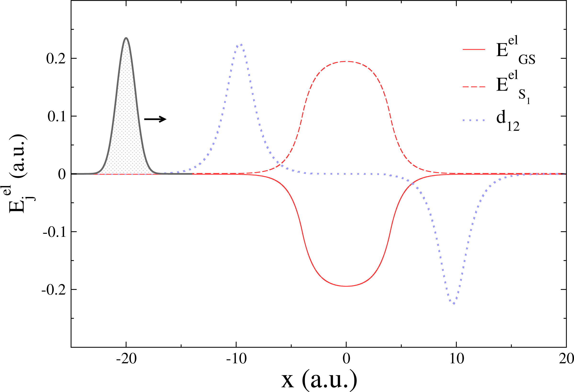
While TSH is an elegant compromise between accuracy and efficiency for the simulation of nonadiabatic phenomena, its accuracy (either in its fewest-switches version or with additional corrections) has been challenged several times in the literature (see [22,68–72] for an non-exhaustive list). Recently, a series of simple one-dimensional model systems were used to highlight potential failures of the standard TSH, even with high initial momenta [28,73–76]. The “double arch” model is composed of a couple of potential energy curves, whose shapes strongly differ in the region where they are not degenerate (−10 ≤ x ≤ 10 a.u. in Figure 1).
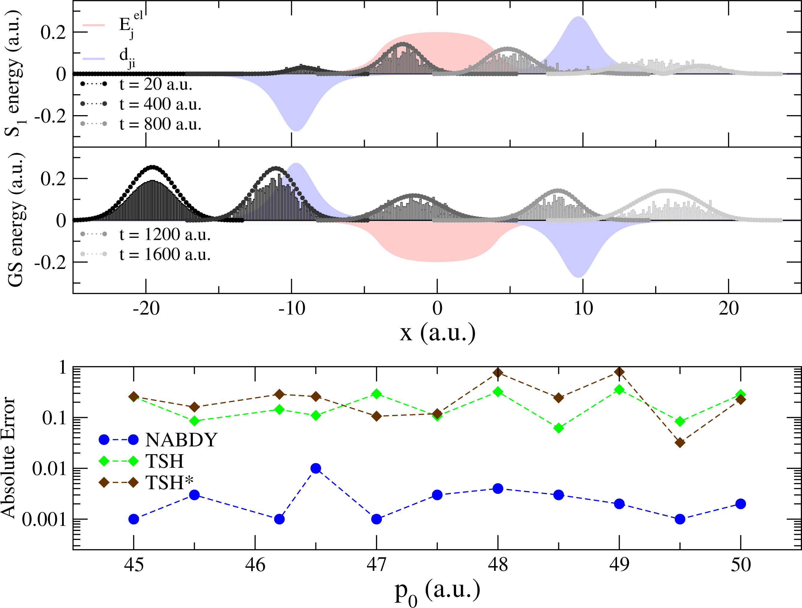
In this model, a Gaussian wave packet launched from x = −20 a.u. with a positive initial momentum will first reach a region of strong nonadiabaticity (Figure 2, upper panel), leading to a population of both the ground state (GS) and the first excited state (S1). Right after this nonadiabatic event occurs, the two potential energy curves will diverge, one exhibiting a strong positive slope (S1 state), the other a negative one (GS). The wave packet contribution in each electronic state will therefore be spatially split and eventually recombined in a second nonadiabatic region at x = 10 a.u. (Figure 2, upper panel). The final population on S1 after the second nonadiabatic region strongly depends on the spatial decoherence between the nuclear wave packets. However, such peculiar decoherence is hardly captured by TSH, due to the independent trajectory approximation (and other approximations discussed in Section 3). This is observed from its deviation with respect to an exact nuclear wave packet propagation in the lower panel of Figure 2. TSH in general fails qualitatively for all different initial momenta tested here, which correspond in all cases to a propagation with no back reflections. Changing the initial conditions of TSH strongly alters the final population of S1, but does not improve it substantially [75]. On the other hand, the correlated quantum trajectories (NABDY) provide an accurate description of the nuclear wave packet propagation with only minor deviations from the exact propagation (full numerical details can be found in [44]).
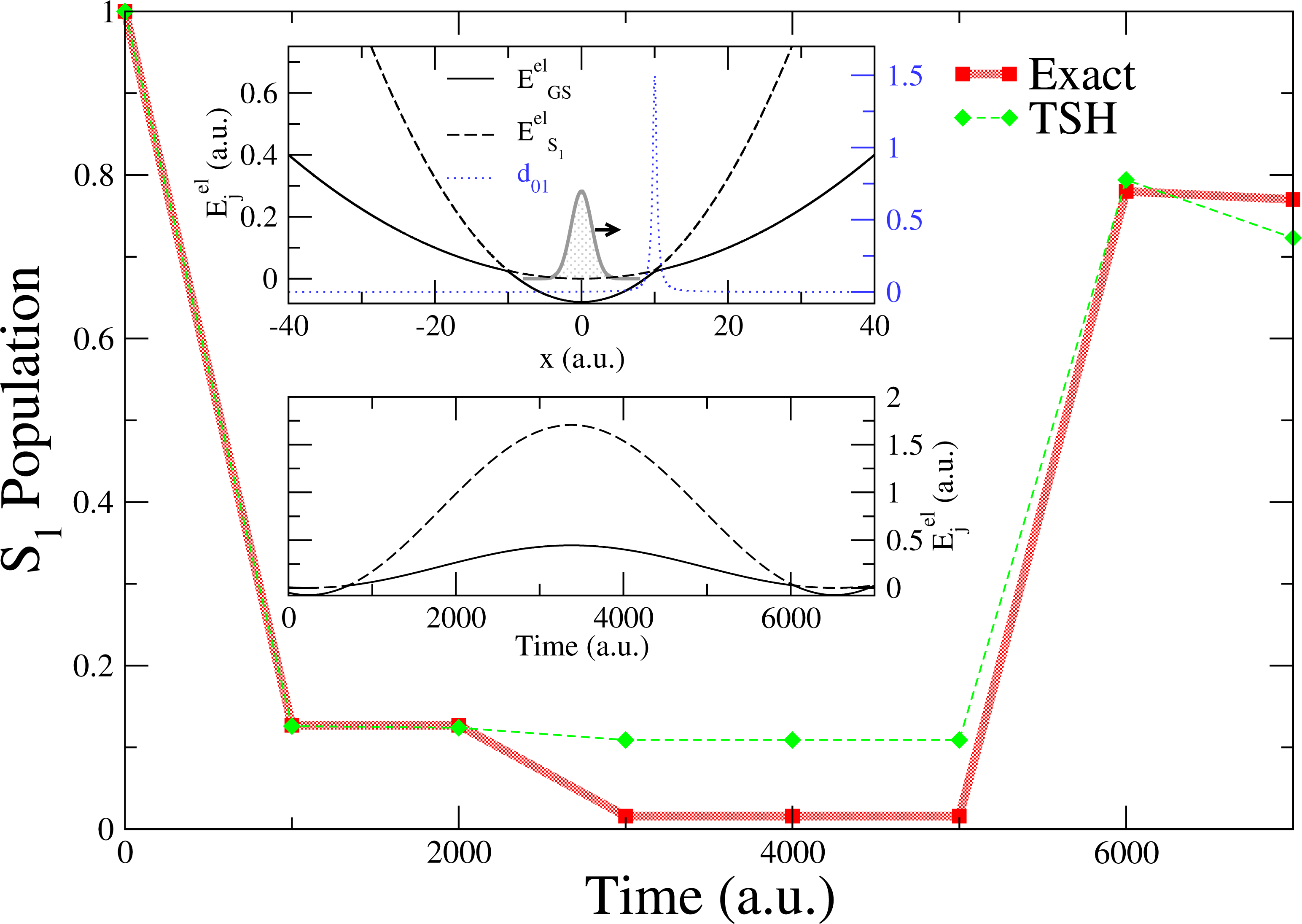
We further investigate the effects of overcoherence on the TSH dynamics by means of a second model system consisting of two coupled harmonic potentials, as depicted in the upper inset of Figure 3. A swarm of trajectories (and a corresponding Gaussian wave packet for the exact propagation) is initialized in the excited state (S1) at x = 0 a.u., with a positive initial momentum p0 = 40 a.u.. In this model system, a single nonadiabatic region is located at x = 10 a.u.; the initial conditions are chosen in such a way that the wave packets (and the classical trajectories) will reflect back shortly after the first transition through the nonadiabatic coupling region, recrossing, therefore, the same coupling region, a second time, with opposite velocity (for a total of two nonadiabatic events, see the lower inset of Figure 3).
The S1 wave packet enters the strong coupling region at x = 10 a.u. (for t < 1, 000 a.u.) and populates the GS (87%, Figure 3). This first nonadiabatic event is perfectly described by TSH (Figure 3, 1000 ≤ t ≤ 2000 a.u.). Due to the difference between the potential energy curves (slope of larger than the one of ), the wave packet component in the GS travels further towards positive x values, while the weak contribution in S1 inverts the direction of its propagation and rapidly returns towards the nonadiabatic region at x = 10 a.u.. In the exact propagation, there is no interference with the wave packet evolving in the GS, since the two wave packets (GS and S1) are spatially separated. As for the first transition through the nonadiabatic region at x ∼10 a.u., the S1 wave packet is transferred almost entirely to the other electronic state (now, the GS, Figure 3, t ≥ 3000 a.u.). On the other hand, in TSH, each independent trajectory carries a set of coherently coupled complex amplitudes (see point (c) of Section 3). When reaching the nonadiabatic coupling at x = 10 a.u. for the second time, the complex amplitudes, and , evolved along a given trajectory, α, in S1, couple coherently, because they share the same support (same position in space for any time t). This induces “overcoherence” in dynamics for the amplitudes, which leads to deviations from the exact propagation (Figure 3, 3000 ≤ t ≤ 5000 a.u.). The total population in S1 increases back to ∼78% of the t = 0 value when the wave packet in the GS recrosses the nonadiabatic region, at t = 6000 a.u.. Some additional deviations of TSH with respect to the exact propagation are observed, and they are linked to subsequent recrossings of the nuclear wave packets.
5. Conclusions
The description of the nonadiabatic dynamics of molecular systems is a challenging task for theory, due to the difficulty of providing both the electronic structure of a system beyond its electronic ground state and the corresponding nuclear dynamics beyond the Born-Oppenheimer approximation. Moreover, nonadiabatic phenomena require a description of the nuclear degrees of freedom that goes beyond the classical approximation, and finally, a good compromise between accuracy and efficiency is also required when realistic molecular systems are investigated. In this article, we have summarized some of the main techniques for describing the nonadiabatic dynamics of molecular systems, namely Ehrenfest dynamics, nonadiabatic Bohmian dynamics, Multiple Spawning, the recently proposed Exact Factorization and trajectory surface hopping. We have also shown how the latter method can be rationalized starting from the “exact” nonadiabatic Bohmian dynamics equations. Trajectory surface hopping is indeed one of the most commonly applied on-the-fly trajectory-based methods to describe the dynamics of molecular systems beyond the Born-Oppenheimer approximation in the (unconstrained) configuration space. This is possible at the cost of describing the nuclear wave packet dynamics with a swarm of uncorrelated classical trajectories with the consequent banishing of all quantum (de)coherence effects. Understanding the underlying limitations of trajectory surface hopping is of foremost importance for the future improvement of the theory, and in our opinion, quantum Bohmian dynamics can give valuable contributions in this direction.
Acknowledgments
We are grateful to Jiří Vaníček and Tomàš Zimmermann for providing us a version of their exact propagation code. COSTactions CM0702 and CM1204 and Swiss National Science Foundation grants 200021-137717 and 200021-146396 are acknowledged for funding and support.
Conflicts of Interest
The authors declare no conflicts of interest.
References and Notes
- Born, M.; Oppenheimer, R. Zur quantentheorie der molekeln. Annalen der Physik 1927, 389, 457–484. (in German). [Google Scholar]
- Ballhausen, C.; Hansen, A. Electronic spectra. Annu. Rev. Phys. Chem 1972, 23, 15–38. [Google Scholar]
- Marx, D.; Hutter, J. Ab Initio Molecular Dynamics: Basic Theory and Advanced Methods; Cambridge University Press: Cambridge, UK, 2009. [Google Scholar]
- Kapral, R.; Ciccotti, G. Mixed quantum-classical dynamics. J. Chem. Phys 1999, 110, 8919–8929. [Google Scholar]
- Tully, J.C. Mixed quantum classical dynamics. Faraday Discuss 1998, 110, 407–419. [Google Scholar]
- Kapral, R. Progress in the theory of mixed quantum-classical dynimics. Annu. Rev. Phys. Chem 2006, 57, 129–157. [Google Scholar]
- Hohenberg, P.; Kohn, W. Inhomogeneous electron gas. Phys. Rev. B 1964, 136, B864–B871. [Google Scholar]
- Kohn, W.; Sham, L.J. Self-consistent equations including exchange and correlation effects. Phys. Rev 1965, 140, A1133–A1138. [Google Scholar]
- Runge, E.; Gross, E.K.U. Density-functional theory for time-dependent systems. Phys. Rev. Lett 1984, 52, 997–1000. [Google Scholar]
- Casida, M.E. Time-dependent density-functional response theory for molecules. In Recent Advances in Density Functional Methods; Chong, D.P., Ed.; World Scientific: Singapore, Singapore, 1995; p. 155. [Google Scholar]
- Petersilka, M.; Gossmann, U.J.; Gross, E.K.U. Excitation energies from time-dependent density-functional theory. Phys. Rev. Lett 1996, 76, 1212–1215. [Google Scholar]
- Appel, H.; Gross, E.K.U.; Burke, K. Excitations in time-dependent density-functional theory. Phys. Rev. Lett 2003, 90, 043005. [Google Scholar]
- Barbatti, M.; Granucci, G.; Ruckenbauer, M.; Plasser, F.; Pittner, J.; Persico, M.; Lischka, H. NEWTON-X, a package for Newtonian dynamics close to the crossing seam, version 1.2, Available online: www.newtonx.org (accessed on 20 December 2013).
- Tully, J.C.; Preston, R.K. Trajectory surface hopping approach to nonadiabatic molecular collisions: The reaction of H+ with D2. J. Chem. Phys 1971, 55, 562–572. [Google Scholar]
- Tully, J.C. Molecular dynamics with electronic transitions. J. Chem. Phys 1990, 93, 1061–1071. [Google Scholar]
- Nielsen, S.; Kapral, R.; Ciccotti, G. Mixed quantum-classical surface hopping dynamics. J. Chem. Phys 2000, 112, 6543–6553. [Google Scholar]
- Herman, M.F. Nonadiabatic semiclassical scattering. I. Analysis of generalized surface hopping procedures. J. Chem. Phys 1984, 81, 754–763. [Google Scholar]
- Sun, X.; Miller, W.H. Semiclassical initial value representation for electronically nonadiabatic molecular dynamics. J. Chem. Phys 1997, 106, 6346–6353. [Google Scholar]
- Coker, D.; Xiao, L. Methods for molecular dynamics with nonadiabatic transitions. J. Chem. Phys 1995, 102, 496–510. [Google Scholar]
- Bittner, E.R.; Rossky, P.J. Quantum decoherence in mixed quantum-classical systems: Nonadiabatic processes. J. Chem. Phys 1995, 103, 8130–8143. [Google Scholar]
- Donoso, A.; Martens, C.C. Simulation of coherent nonadiabatic dynamics using classical trajectories. J. Phys. Chem. A 1998, 102, 4291–4300. [Google Scholar]
- Horenko, I.; Salzmann, C.; Schmidt, B.; Schutte, C. Quantum-classical Liouville approach to molecular dynamics: Surface hopping Gaussian phase-space packets. J. Chem. Phys 2002, 117, 11075–11088. [Google Scholar]
- Burghardt, I.; Cederbaum, L. Hydrodynamic equations for mixed quantum states. II. Coupled electronic states. J. Chem. Phys 2001, 115, 10312–10322. [Google Scholar]
- Bonella, S.; Coker, D.F. LAND-map, a linearized approach to nonadiabatic dynamics using the mapping formalism. J. Chem. Phys 2005, 122, 194102. [Google Scholar]
- McEniry, E.J.; Wang, Y.; Dundas, D.; Todorov, T.N.; Stella, L.; Miranda, R.P.; Fisher, A.J.; Horsfield, A.P.; Race, C.P.; Mason, D.R.; et al. Modelling non-adiabatic processes using correlated electron-ion dynamics. Eur. Phys. J. B 2010, 77, 305–329. [Google Scholar]
- Thachuk, M.; Ivanov, M.Y.; Wardlaw, D.M. A semiclassical approach to intense-field above-threshold dissociation in the long wavelength limit. II. Conservation principles and coherence in surface hopping. J. Chem. Phys 1998, 109, 5747–5760. [Google Scholar]
- Fang, J.Y.; Hammes-Schiffer, S. Improvement of the internal consistency in trajectory surface hopping. J. Phys. Chem. A 1999, 103, 9399–9407. [Google Scholar]
- Subotnik, J.; Shenvi, N. A new approach to decoherence and momentum rescaling in the surface hopping algorithm. J. Chem. Phys 2011, 134, 024105. [Google Scholar]
- Meyer, H.D.; Manthe, U.; Cederbaum, L.S. The multi-configurational time-dependent hartree approach. Chem. Phys. Lett 1990, 165, 73–78. [Google Scholar]
- Bohm, D. A suggested interpretation of the quantum theory in terms of “hidden” variables. I. Phys. Rev 1952, 85, 166–179. [Google Scholar]
- Bohm, D. A suggested interpretation of the quantum theory in terms of “hidden” variables. II. Phys. Rev 1952, 85, 180–193. [Google Scholar]
- Takabayasi, T. On the formulation of quantum mechanics associated with classical pictures. Prog. Theor. Phys 1952, 8, 143–182. [Google Scholar]
- Holland, P.R. The Quantum Theory of Motion—An Account of the de Broglie-Bohm Causal Interpretation of Quantum Mechanics; Cambridge University Press: Cambridge, UK, 1993. [Google Scholar]
- Lopreore, C.L.; Wyatt, R.E. Quantum wave packet dynamics with trajectories. Phys. Rev. Lett 1999, 82, 5190–5193. [Google Scholar]
- Wyatt, R.E. Quantum Dynamics with Trajectories: Introduction to Quantum Hydrodynamics; interdisciplinary applied mathematics; Springer: New York, NY, USA, 2005. [Google Scholar]
- Chattaraj, P.K., Ed.; Quantum Trajectories; Atoms, Molecules, and Clusters Series; CRC Press: Boca Raton, FL, USA, 2010.
- Oriols, X., Mompart, J., Eds.; Applied Bohmian Mechanics, From Nanoscale Systems to Cosmology; Pan Stanford Publishing Pte. Ltd.: Singapore, Singapore, 2012.
- Wyatt, R.E.; Lopreore, C.L.; Parlant, G. Electronic transitions with quantum trajectories. J. Chem. Phys 2001, 114, 5113–5116. [Google Scholar]
- Lopreore, C.L.; Wyatt, R.E. Electronic transitions with quantum trajectories. II. J. Chem. Phys 2002, 116, 1228–1238. [Google Scholar]
- Gindensperger, E.; Meier, C.; Beswick, J.; Parlant, G. Combining fixed-and moving-grid methods to study direct dissociation processes involving nonadiabatic transitions. J. Chem. Phys 2005, 123, 214107. [Google Scholar]
- Poirier, B.; Parlant, G. Reconciling semiclassical and Bohmian mechanics: IV. Multisurface dynamics. J. Phys. Chem. A 2007, 111, 10400–10408. [Google Scholar]
- Garashchuk, S.; Rassolov, V.A.; Schatz, G.C. Semiclassical nonadiabatic dynamics using a mixed wave-function representation. J. Chem. Phys 2005, 123, 174108. [Google Scholar]
- Curchod, B.F.E.; Tavernelli, I.; Rothlisberger, U. Trajectory-based solution of the nonadiabatic quantum dynamics equations: An on-the-fly approach for molecular dynamics simulations. Phys. Chem. Chem. Phys 2011, 13, 3231–3236. [Google Scholar]
- Curchod, B.F.E.; Tavernelli, I. On trajectory-based nonadiabatic dynamics: Bohmian dynamics versus trajectory surface hopping. J. Chem. Phys 2013, 138, 184112. [Google Scholar]
- Martínez, T.J.; Ben-Nun, M.; Levine, R.D. Multi-electronic-state molecular dynamics: A wave function approach with applications. J. Phys. Chem 1996, 100, 7884–7895. [Google Scholar]
- Martínez, T.J.; Ben-Nun, M.; Levine, R.D. Molecular collision dynamics on several electronic states. J. Phys. Chem. A 1997, 101, 6389–6402. [Google Scholar]
- Martínez, T.J.; Levine, R.D. Non-adiabatic molecular dynamics: Split-operator multiple spawning with applications to photodissociation. J. Chem. Soc. Faraday Trans 1997, 93, 941–947. [Google Scholar]
- Ben-Nun, M.; Martínez, T.J. Nonadiabatic molecular dynamics: Validation of the multiple spawning method for a multidimensional problem. J. Chem. Phys 1998, 108, 7244–7257. [Google Scholar]
- Born, M. Kopplung der Elektronen- und Kernbewegung in Molekeln und Kristallen; (in German). Vandenhoeck & Ruprecht: Göttingen, Germany, 1951. [Google Scholar]
- Born, M.; Huang, K. Dynamical Theory of Crystal Lattices; Clarendon: Oxford, UK, 1954. [Google Scholar]
- The term “Born-Oppenheimer approximation” is also used to name what should be referred to as the “adiabatic BO approximation”.
- Ben-Nun, M.; Martínez, T.J. Ab Initio Quantum Molecular Dynamics. In Advances in Chemical Physics; Volume 121, Wiley: New York, NY, USA, 2002; pp. 439–512. [Google Scholar]
- The spawning process is rather involved, and the interested reader should refer to [52] for a very detailed discussion of the algorithm.
- Ben-Nun, M.; Quenneville, J.; Martínez, T.J. Ab initio multiple spawning: Photochemistry from first principles quantum molecular dynamics. J. Phys. Chem. A 2000, 104, 5161–5175. [Google Scholar]
- For an in-depth discussion on Bohmian mechanics and its physical meaning, see [33].
- Tavernelli, I. Ab initio–driven trajectory-based nuclear quantum dynamics in phase space. Phys. Rev. A 2013, 87, 042501. [Google Scholar]
- Tully, J.C. Nonadiabatic Dynamics. In Modern Methods for Multidimensional Dynamics Computations in Chemistry; Thompson, D.L., Ed.; World Scientific: Singapore, Singapore, 1998. [Google Scholar]
- Tavernelli, I. Electronic density response of liquid water using time-dependent density functional theory. Phys. Rev. B 2006, 73, 094204. [Google Scholar]
- Abedi, A.; Maitra, N.; Gross, E. Exact factorization of the time-dependent electron-nuclear wave function. Phys. Rev. Lett 2010, 105, 123002. [Google Scholar]
- Abedi, A.; Maitra, N.T.; Gross, E. Correlated electron-nuclear dynamics: Exact factorization of the molecular wavefunction. J. Chem. Phys 2012, 137, 22A530. [Google Scholar]
- Hunter, G. Conditional probability amplitudes in wave mechanics. Int. J. Quantum Chem 1975, 9, 237–242. [Google Scholar]
- Alonso, J.L.; Clemente-Gallardo, J.; Echenique-Robba, P.; Jover-Galtier, J.A. Comment on “Correlated electron-nuclear dynamics: Exact factorization of the molecular wavefunction” (J. Chem. Phys.137, 22A530 (2012)). J. Chem. Phys. 2013, 139, 087101. [Google Scholar]
- Abedi, A.; Maitra, N.T.; Gross, E.K.U. Response to: Comment on “Correlated electron-nuclear dynamics: Exact factorization of the molecular wavefunction” (J. Chem. Phys. 139, 087101 (2013)). J. Chem. Phys. 2013, 139, 087102. [Google Scholar]
- Barbatti, M.; Shepard, R.; Lischka, H. Computational and methodological elements for nonadiabatic trajectory dynamics simulations of molecules. In Conical Intersections: Theory, Computation and Experiment; Domcke, W., Yarkony, D.R., Koeppel, H., Eds.; World Scientific: Singapore, Singapore, 2011; p. 415. [Google Scholar]
- Barbatti, M. Nonadiabatic dynamics with trajectory surface hopping method. WIREs Comput. Mol. Sci 2011, 1, 620–633. [Google Scholar]
- Curchod, B.F.E.; Rothlisberger, U.; Tavernelli, I. Trajectory-based nonadiabatic dynamics with time-dependent density functional theory. Chem. Phys. Chem 2013, 14, 1314–1340. [Google Scholar]
- Burant, J.C.; Tully, J.C. Nonadiabatic dynamics via the classical limit Schrödinger equation. J. Chem. Phys 2000, 112, 6097. [Google Scholar]
- Granucci, G.; Persico, M. Critical appraisal of the fewest switches algorithm for surface hopping. J. Chem. Phys 2007, 126, 134114–11. [Google Scholar]
- Worth, G.A.; Hunt, P.; Robb, M.A. Nonadiabatic dynamics: A comparison of surface hopping direct dynamics with quantum wave packet calculations. J. Phys. Chem. A 2003, 107, 621–631. [Google Scholar]
- Herman, M.F.; Moody, M.P. Numerical study of the accuracy and efficiency of various approaches for Monte Carlo surface hopping calculations. J. Chem. Phys 2005, 122, 094104. [Google Scholar]
- Granucci, G.; Persico, M.; Zoccante, A. Including quantum decoherence in surface hopping. J. Chem. Phys 2010, 133, 134111. [Google Scholar]
- Richter, M.; Marquetand, P.; González-Vázquez, J.; Sola, I.; González, L. SHARC: Ab Initio molecular dynamics with surface hopping in the adiabatic representation including arbitrary couplings. J. Chem. Theory Comput 2011, 7, 1253–1258. [Google Scholar]
- Shenvi, N.; Subotnik, J.; Yang, W. Phase-corrected surface hopping: Correcting the phase evolution of the electronic wavefunction. J. Chem. Phys 2011, 135, 024101. [Google Scholar]
- Subotnik, J.; Shenvi, N. Decoherence and surface hopping: When can averaging over initial conditions help capture the effects of wave packet separation? J. Chem. Phys 2011, 134, 244114. [Google Scholar]
- Shenvi, N.; Subotnik, J.; Yang, W. Simultaneous-trajectory surface hopping: A parameter-free algorithm for implementing decoherence in nonadiabatic dynamics. J. Chem. Phys 2011, 134, 144102. [Google Scholar]
- Shenvi, N.; Yang, W. Achieving partial decoherence in surface hopping through phase correction. J. Chem. Phys 2012, 137. [Google Scholar] [CrossRef]


© 2014 by the authors; licensee MDPI, Basel, Switzerland This article is an open access article distributed under the terms and conditions of the Creative Commons Attribution license (http://creativecommons.org/licenses/by/3.0/).
Share and Cite
De Carvalho, F.F.; Bouduban, M.E.F.; Curchod, B.F.E.; Tavernelli, I. Nonadiabatic Molecular Dynamics Based on Trajectories. Entropy 2014, 16, 62-85. https://doi.org/10.3390/e16010062
De Carvalho FF, Bouduban MEF, Curchod BFE, Tavernelli I. Nonadiabatic Molecular Dynamics Based on Trajectories. Entropy. 2014; 16(1):62-85. https://doi.org/10.3390/e16010062
Chicago/Turabian StyleDe Carvalho, Felipe Franco, Marine E. F. Bouduban, Basile F. E. Curchod, and Ivano Tavernelli. 2014. "Nonadiabatic Molecular Dynamics Based on Trajectories" Entropy 16, no. 1: 62-85. https://doi.org/10.3390/e16010062
APA StyleDe Carvalho, F. F., Bouduban, M. E. F., Curchod, B. F. E., & Tavernelli, I. (2014). Nonadiabatic Molecular Dynamics Based on Trajectories. Entropy, 16(1), 62-85. https://doi.org/10.3390/e16010062