Abstract
Existing algorithms for learning Boolean networks (BNs) have time complexities of at least O(N·n0.7(k+1)), where n is the number of variables, N is the number of samples and k is the number of inputs in Boolean functions. Some recent studies propose more efficient methods with O(N·n2) time complexities. However, these methods can only be used to learn monotonic BNs, and their performances are not satisfactory when the sample size is small. In this paper, we mathematically prove that OR/AND BNs, where the variables are related with logical OR/AND operations, can be found with the time complexity of O(k·(N + logn)·n2), if there are enough noiseless training samples randomly generated from a uniform distribution. We also demonstrate that our method can successfully learn most BNs, whose variables are not related with exclusive OR and Boolean equality operations, with the same order of time complexity for learning OR/AND BNs, indicating our method has good efficiency for learning general BNs other than monotonic BNs. When the datasets are noisy, our method can still successfully identify most BNs with the same efficiency. When compared with two existing methods with the same settings, our method achieves a better comprehensive performance than both of them, especially for small training sample sizes. More importantly, our method can be used to learn all BNs. However, of the two methods that are compared, one can only be used to learn monotonic BNs, and the other one has a much worse time complexity than our method. In conclusion, our results demonstrate that Boolean networks can be learned with improved time complexities.
1. Introduction
Gene Regulatory Networks (GRNs) are believed to be the underlying mechanisms that control different gene expression patterns. Every regulatory module in the genome receives multiple disparate inputs and processes them in ways that can be mathematically represented as combinations of logical functions (e.g., “AND” functions, “SWITCH” functions, and “OR” functions) [1]. Then, different regulatory modules are weaved together into complex GRNs, which give specific outputs, i.e., different gene expression patterns (like in developmental processes), depending on their inputs, i.e., the current status of the cell. Hence, the architecture of GRN is fundamental for both explaining and predicting developmental phenomenology [2,3].
Boolean networks (BNs) [4] as models have received much attention in reconstructing GRNs from gene expression data sets [5,6,7,8,9,10,11,12,13,14,15,16,17,18,19,20,21]. Many algorithms are computationally expensive, with their complexities on the order of , as summarized in Table 1. Liang et al. [13] proposed the REVEALalgorithm, with complexity, to reconstruct BNs from binary transition pairs. Akutsu et al. [5] introduced an algorithm for the same purpose, but the complexity of their method is , which is worse than that of REVEAL. Akutsu et al. [6] proposed another algorithm with a complexity of , where to find the BNs with high probability. Schmulevich et al. [19,20] introduced an algorithm with a complexity of . Lähdesmäki et al. [12] proposed an algorithm with complexity, where is k in most cases. Laubenbacher and Stigler [11] proposed a method based on algebra with a complexity of , where p is the size of the state set, S, and c is a constant. Nam et al. [18] proposed a method with an average time complexity of . Kim et al. [10] introduced an algorithm with , where is the number of first selected genes for the jth gene and is the number of second selected genes when the ith gene is selected in the first step.
In the field of machine learning, there are also many algorithms introduced for learning Boolean functions [22,23,24,25,26,27,28,29,30]. If these algorithms are modified to learning BNs of a bounded indegree of k, i.e., n Boolean functions with k inputs, their complexities are at least .
More efficient algorithms are indispensable to simulate GRNs with BNs on a large scale. Akutsu et al. [8] proposed an approximation algorithm called GREEDY1with the complexity of , but the success ratio of the GREEDY1 algorithm is not satisfactory, especially when k is small. For example, the success ratio of the GREEDY1 algorithm is only around 50%, no matter how many learning samples are used when k = 2 for the general Boolean functions. An efficient algorithm was also proposed by Mossel et al. [31] with a time complexity of , which is about , for learning arbitrary BNs, where . Arpe and Reischuk [32] showed that monotonic BNs could be learned with a complexity of under -bounded noise. A Boolean function is monotonic if for every input variable, the function is either monotonically increasing or monotonically decreasing in that variable [16]. Recently, Maucher et al. [16] proposed an efficient method with a time complexity of . However, this method, as well as its improvement in [17], is only applicable to BNs containing only monotonic Boolean functions, and its specificity is unsatisfactory when the sample size is small. In our work [21], we introduced the Discrete Function Learning (DFL) algorithm with the expected complexity of for reconstructing qualitative models of GRNs from gene expression datasets.

Table 1.
The summary of the complexities of different algorithms for learning BNs.
| Time Complexity | Reference |
|---|---|
| [13] | |
| [5] | |
| , where | [6] |
| [19,20] | |
| [12] | |
| [11] | |
| , where | [31] |
| [18] | |
| [32] | |
| [10] | |
| [16] |
* for BNs of monotonic Boolean functions.
Until now, there is still an open question about learning general BNs with a complexity better than [31,32]. In this work, as an endeavor to meet the challenge, we prove that the complexity of the DFL algorithm is strictly for learning the OR/AND BNs in the worst case, given enough noiseless random samples from the uniform distribution. This conclusion is also validated through comprehensive experiments. We also demonstrate that the complexity of the DFL algorithm is still for learning general BNs, whose input variables are not related with exclusive OR (XOR) and Boolean equality (the inversion of exclusive OR, also called XNOR) operations. Even for exclusive OR and Boolean equality functions, the DFL algorithm can still correctly identify the original networks, although it uses more time, with the worst case complexity of . Furthermore, even when the datasets are noisy, the DFL algorithm shows a more competitive performance than the existing methods in [12,16] without losing its efficiency, especially when the sample size is small.
2. Background and Theoretical Foundation
We first introduce the notation. We use capital letters to represent random variables, such as X and Y, lower case letters to represent an instance of the random variable, such as x and y, bold capital letters, like X, to represent a set of variables, and lower case bold letter, like x, to represent an instance of X. and mean the estimations of probability P and mutual information (MI) I using the training samples, respectively. In Boolean functions, we use “∨”, “∧”, “¬”, “⨁” and “≡” to represent logical OR, AND, INVERT (also named NOT or SWITCH), exclusive OR (XOR) and Boolean equality (the inversion of exclusive OR, also XNOR), respectively. For the purpose of simplicity, we represent with , with , and so on. We use log to stand for log2, where its meaning is clear. We use to mean the ith selected input variable of the function to be learned.
In this section, we first introduce BN as a model of GRN. Then, we cover some preliminary knowledge of information theory. Next, we introduce the theoretical foundation of our method. The formal definition of the problem of learning BNs and the quantity of data sets are discussed in the following.
2.1. BN as a Model of GRN
In qualitative models of GRNs, the genes are represented by a set of discrete variables, . In GRNs, the expression level of a gene, X, at time step, t + 1, is controlled by the expression levels of its regulatory genes, which encode the regulators of the gene, X, at time step t. Hence, in qualitative models of GRNs, the genes at the same time step are assumed to be independent of each other, which is a standard assumption in learning GRNs, as adopted by [5,6,8,12,13,21]. Formally, , and are independent. Additionally, the regulatory relationships between the genes are expressed by discrete functions related to variables. Formally, a GRN with indegree k (the number of inputs) consists of a set, , of nodes representing genes and a set, , of discrete functions, where a discrete function, , with inputs from specified nodes, , at time step t is assigned to the node, , to calculate its value at time step . As shown in the following equation:
where and to mean the jth selected input variable of the function related to . We call the inputs of the parent nodes of , and let .
The state of the GRN is expressed by the state vector of its nodes. We use to represent the state of the GRN at time t and to represent the state of the GRN at time . is calculated from with F. A state transition pair is . Hereafter, we use to represent , to represent , to represent , and so on.
When s in Equation (1) are Boolean functions, i.e., , the is a BN model [4,5,21]. When using BNs to model GRNs, genes are represented with binary variables with two values: ON (1) and OFF (0).
2.2. Preliminary Knowledge of Information Theory
The entropy of a discrete random variable, X, is defined in terms of the probability of observing a particular value, x, of X as [33]:
The entropy is used to describe the diversity of a variable or vector. The more diverse a variable or vector is, the larger entropy it has. Generally, vectors are more diverse than individual variables; hence, they have larger entropy. The MI between a vector, X, and Y is defined as [33]:
MI is always non-negative and can be used to measure the relation between two variables, a variable and a vector (Equation (3)) or two vectors. Basically, the stronger the relation between two variables is, the larger MI they have. Zero MI means that the two variables are independent or have no relation. Formally:
Theorem 1
([34](p. 27)) For any discrete random variables, Y and Z, . Moreover, , if and only if Y and Z are independent.
The conditional MI, [34](the MI between X and Y given Z), is defined by:
Immediately from Theorem 1, the following corollary is also correct.
Corollary 1
([34](p. 27)) with equality, if and only if Z and Y are conditionally independent given X.
Here, conditional independence is introduced in [35].
The conditional entropy and entropy are related to Theorem 2.
Theorem 2
([34](p. 27)) with equality, if and only if X and Y are independent.
The chain rule for MI is given by Theorem 3.
Theorem 3
([34](p. 22))
In a function, we have the following theorem.
Theorem 4
([36](p. 37)) If , then .
2.3. Theoretical Foundation of The DFL Algorithm
Next, we introduce Theorem 5, which is the theoretical foundation of our algorithm.
Theorem 5
([34](p. 43)) If the mutual information between X and Y is equal to the entropy of Y, i.e., , then Y is a function of X.
In the context of inferring BNs from state transition pairs, we let with (), and . The entropy, , represents the diversity of the variable, Y. The MI, , represents the relation between vector X and Y. From this point of view, Theorem 5 actually says that the relation between vector X and Y is very strong, such that there is no more diversity for Y if X has been known. In other words, the value of X can fully determine the value of Y.
In practice, the empirical probability (or frequency), the empirical entropy and MI estimated from a sample may be biased, since the number of experiments is limited. Thus, let us restate Borel’s law of large numbers about the empirical probability, .
Theorem 6
(Borel’s Law of Large Numbers)
where is the number of instances in which .
From Theorem 6, it is known that if enough samples, , as well as and , can be correctly estimated, which ensures the successful usage of Theorem 5 in practice.
We discuss the probabilistic relationship between X, Y and another vector, .
Theorem 7
(Zheng and Kwoh, [37]) If , , Y and Z are conditionally independent given X.
Immediately from Theorem 7 and Corollary 1, we have Corollary 2.
Corollary 2
If , , , then .
Theorem 7 says that if there is a subset of features, X, that satisfies , the remaining variables in V do not provide additional information about Y, once we know X. If Z and X are independent, we can further have Theorem 8, whose proof is given in the Appendix.
Theorem 8
If , and X and Z are independent, then .
In the context of BNs, remember that , and in V are independent. Thus, , Z and are independent.
2.4. Problem Definition
Technological development has made it possible to obtain time series gene expression profiles with microarray [38] and high-throughput sequencing (or RNA-seq) [39]. The time series gene expression profiles can thus be organized as input-output transition pairs whose inputs and outputs are the expression profile of time t and , respectively [6,13]. The problem of inferring the BN model of the GRN from input-output transition pairs is defined as follows.
Definition 1
(Inference of the BN) Let . Given a transition table, , where j goes from one to a constant, N, find a set of Boolean functions , so that is calculated from as follows:
Akutsu et al. [6] stated another set of problems for inferring BNs. The CONSISTENCY problem defined in [6] is to determine whether or not there exists a Boolean network consistent with the given examples and an output of one if it exists. Therefore, the CONSISTENCY problem is the same as the one in Definition 1.
2.5. Data Quantity
Akutsu et al. [5] proved that transition pairs are the theoretic lower bound to learn a BN. Formally:
Theorem 9
(Akutsu et al. [5]) transition pairs are necessary in the worst case to identify the Boolean network of maximum indegree ≤ k.
3. Methods
In this section, we briefly reintroduce the DFL algorithm, which can efficiently find the target subsets from subsets of V with less than or equal to k variables. The detailed steps, the analysis of complexities and the correctness of the DFL algorithm are stated in our early work [21,37,40].
3.1. A Brief Introduction of the DFL Algorithm
Based on Theorem 5, the motivation of the DFL algorithm is to find a subset of features that satisfies . To efficiently fulfill this purpose, the DFL algorithm employs a special searching strategy to find the expected subset. In the first round of its searching, the DFL algorithm uses a greedy strategy to incrementally identify real relevant feature subsets, U, by maximizing [37]. However, in some special cases, such as the exclusive OR functions, individual real input features have zero MI with the output feature, although for a vector, X, with all real input variables, is still correct in these special cases. Thus, in these cases, after the first k features, which are not necessarily the true inputs, are selected, a simple greedy search fails to identify the correct inputs with a high probability. Therefore, the DFL algorithm continues its searching until it checks all subsets with ≤ k variables after the first round of greedy searching. This strategy guarantees the correctness of the DFL algorithm even if the input variables have special relations, such as exclusive OR.
The main steps of the DFL algorithm are listed in Table 2 and Table 3. The DFL algorithm has two parameters, the expected cardinality, k, and the ϵ value. The k is the expected maximum number of inputs in the GRN models. The DFL algorithm uses the k to prevent the exhaustive searching of all subsets of attributes by checking those subsets less than or equal to k variables. The ϵ value will be discussed below and has been introduced in detail in our early work [21,37,40].
Table 2.
The Discrete Function Learning (DFL) algorithm.
| Algorithm: DFL(V, k, T) | |
| Input: V with n genes, indegree k, T = {(V(t), V(t + 1))}, t = 1, …, N. | |
| Output: F = {f1, f2, …, fn} | |
| Begin: | |
| 1 | L ← all single element subsets of V; |
| 2 | ΔTree.FirstNode ← L |
| 3 | for every gene Y ∈ V { |
| 4 | calculate H(Y′); //from T |
| 5 | D ← 1; //initial depth |
| 6 * | F. Add (Sub(Y, ΔTree, H(Y′), D, k)); |
| } | |
| 7 | return F; |
| End |
* The Sub() is a sub-routine listed in Table 3.
From Theorem 5, if an input subset, , satisfies , then Y is a deterministic function of U, which means that U is a complete and optimal input subset. U is called essential attributes (EAs), because U essentially determines the value of Y [41].
In real life, datasets are often noisy. The noise changes the distributions of X and Y; therefore , and are changed, due to the noise. Thus, the in Theorem 5 is disrupted. In these cases, we have to relax the requirement to obtain the best estimated result. Therefore, ϵ is defined as a significance factor to control the difference between and . Precisely, if a subset, U, satisfies , then the DFL algorithm stops the searching process and uses U as a best estimated subset. Accordingly, line 4 of Table 3 should be modified.
Table 3.
The sub-routine of the DFL algorithm.
| Algorithm: Sub(Y, ΔTree, H, D, k) | |
| Input: Y, ΔTree, entropy H(Y) | |
| current depth D, indegree k | |
| Output: function Y = f(X) | |
| Begin: | |
| 1 | L ← ΔTree.DthNode; |
| 2 | for every element X ∈ L { |
| 3 | calculate I(X; Y); |
| 4 | if(I(X; Y) == H) { |
| 5 * | extract Y = f(X) from T; |
| 6 | return Y = f(X); |
| } | |
| } | |
| 7 | sort L according to I; |
| 8 | for every element X ∈ L { |
| 9 | if(D < k){ |
| 10 | D ← D + 1; |
| 11 | ΔTree.DthNode ← Δ1(X); |
| 12 | return Sub(Y, ΔTree, H, D, k); |
| } | |
| } | |
| 13 | return “Fail(Y)”; |
| End |
* By deleting unrelated variables and duplicate rows in T.
When choosing candidate inputs, our approach maximizes the MI between the input subsets, X, and the output attribute, Y. Suppose that has already been selected at step , and the DFL algorithm tries to add a new input to . Specifically, our method uses Equation (4) as a criterion to add new features to U.
where , , , and .
To illustrate the searching strategy used by the DFL algorithm, let us consider a BN consisting of four genes, as shown in Table 4. The set of all genes is . The search procedure of the DFL algorithm to find the Boolean function of of the example in Table 4 is shown in Figure 1. The DFL algorithm uses a data structure called in its calculation [37]. For instance, the when the DFL algorithm is learning is shown in Figure 2. As shown in Figure 1, the DFL algorithm searches the first layer, , then it sorts all subsets according to their MI with on . From Theorem 8, A, C and D have larger MI with than B has. Consequently, the DFL algorithm finds that shares the largest MI with among subsets on , as shown in Figure 2a. Next, one additional variable is added to the selected A. Similarly to , the DFL algorithm finds that shares the largest MI with on , as shown in Figure 2b. Then, the DFL algorithm adds one more variable to the selected . Finally, the DFL algorithm finds that the subset, , satisfies the requirement of Theorem 5, as shown in Figure 2c, and constructs the function, f, for with these three attributes. First, B is deleted from the training dataset, since it is a non-essential attribute. Then, the duplicate rows of are removed from the training dataset to obtain the final function, f, as the truth table of along with the counts for each instance of . This is the reason for which we name our algorithm the Discrete Function Learning algorithm.
Table 4.
Boolean functions, , of the example.
| Gene | Rule |
|---|---|
| A | A′ = B |
| B | B′ = A ∨ C |
| C | C′ = A ∨ C ∨ D |
| D | D′ = (A ∧ B) ∨ (C ∧ D) |
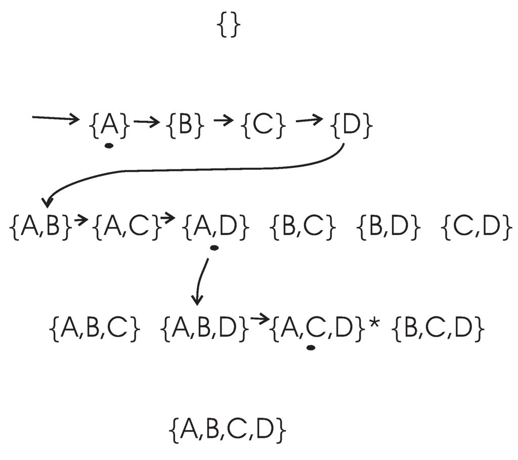
Figure 1.
Search procedures of the DFL algorithm when learning . is the target combination. The combinations with a black dot under them are the subsets that share the largest mutual information (MI) with on their layers. Firstly, the DFL algorithm searches the first layer, , then finds that , with a black dot under it, shares the largest MI with among subsets on the first layer. Then, it continues to search (subsets with A and another variable) on the second layer, . Similarly, these calculations continue, until the target combination, , is found on the third layer, .
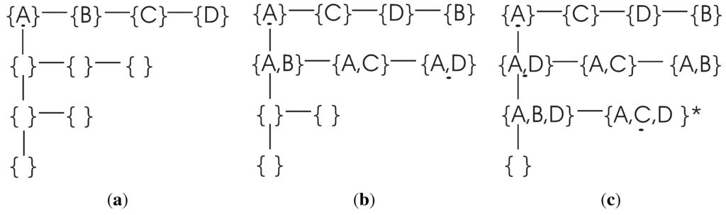
Figure 2.
The ΔTree when searching the Boolean functions for (a) after searching the first layer of V, but before the sort step; (b) when searching the second layer of V (the , and , which are included in the , are listed before after the sort step); (c) when searching the third layer; is the target combination. Similar to part (b), the and are listed before . When checking the combination, , the DFL algorithm finds that is the complete parent set for , since satisfies the criterion of Theorem 5.
3.2. Correctness Analysis
We have proven the following theorem [37].
Theorem 10
(Zheng and Kwoh, [37]) Let . The DFL algorithm can find a consistent function, , of maximum indegree k with time in the worst case from .
The word “consistent” means that the function is consistent with the learning samples, i.e., . Clearly, the original generating function of a synthetic dataset is a consistent function of the synthetic dataset.
From Theorem 5, to solve the problem in Definition 1 is actually to find a group of genes , so that the MI between and is equal to the entropy of . Because n functions should be learned in Definition 1, the total time complexity is in the worst case, based on Theorem 10.
4. The Time Complexity for Learning Some Special BNs
In this section, we first analyze the MI between variables in some special BNs where variables are related with the logical OR(AND) operations. Then, we propose the theorems about the complexities of the DFL algorithm for learning these BNs. The proofs of the theorems in this section are given in the Appendix.
It should be mentioned that because the real functional relations between variables are unknown in prior, it is infeasible to specifically design an algorithm just for one kind of special BN. Although some special BNs are discussed in this section, the DFL algorithm can be used to learn all BNs without knowing the real functional relations between variables a priori.
4.1. The MI in OR BNs
Formally, we define the OR BN as follows.
Definition 2
The OR BN of a set of binary variables is :
where the “∨” is the logical OR operation.
We have Theorem 11 to compute the in OR BNs.
Theorem 11
In an OR BN with an indegree of k over V, the mutual information between and is:
From Equation (6), we see that is strictly positive and tends to be zero when , as shown in Figure 3a. Intuitively, when k increases, there would be more “1” values in the column of the truth table, while only one “0” whatever value the k is. That is to say, tends to take the value of “1” with higher probability or there are less uncertainties in when k increases, which causes to decrease. From Theorem 4, ; thus, also decreases. Therefore, each shares less information with when k increases.
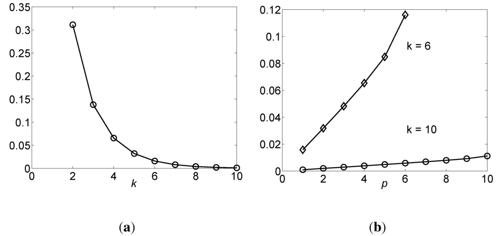
Figure 3.
MI in OR function , where the unit of MI (vertical axis) is a bit. (a) The as a function of k, ; (b) as a function of p, where , and p goes from 1 to k.
Similar to Theorem 11, we have Theorem 12 for computing , where . From Theorem 12, we further have Theorem 13.
Theorem 12
In an OR BN with an indegree of k over V, , , the mutual information between and is:
Theorem 13
In an OR BN with indegree of k over V, , .
From Theorem 13, it is known that when variables from are added to the candidate parent set, U, for , the MI, , increases, which is also shown in Figure 3b.
4.2. The Complexity Analysis for the Bounded OR BNs
Theorems 11 to 13 show theoretical values. When learning BNs from a training dataset with limited samples, the estimation of MI is affected by how the samples are obtained. Here, we assume that the samples are generated randomly from a uniform distribution. According to Theorem 9, transition pairs are necessary to successfully identify the BNs of ≤ k inputs. Then, based on Theorem 6, if enough samples are provided, the distributions of and tend to be those in the truth table of . We then obtain the following theorem.
Theorem 14
For sufficiently large , if the samples are noiseless and randomly generated from a uniform distribution, then the DFL algorithm can identify an OR BN with an indegree of k in time, strictly.
Enough learning samples are required in Theorem 14. If the sample size is small, it is possible that variables in do not share larger MI than variables in do. As will be discussed in the Discussion section and Figure 4, it is shown that when N = 20, . However, in this example, so it takes more steps before the DFL algorithm finally finds the target subset of . Therefore, the complexity of the DFL algorithm becomes worse than if N is too small, as will be shown in Figure 9.
If some variables take their inverted values in the OR BNs, these kinds of BNs are defined as generalized OR BNs.
Definition 3
The generalized OR BN of a set of binary variables is, :
where the “∨” is the logical OR operation; can also take their inverted values.
For generalized OR BNs, the DFL algorithm also maintains its time complexity of .
Corollary 3
For sufficiently large , if the samples are noiseless and randomly generated from a uniform distribution, then the DFL algorithm can identify a generalized OR BN with an indegree of k in time, strictly.
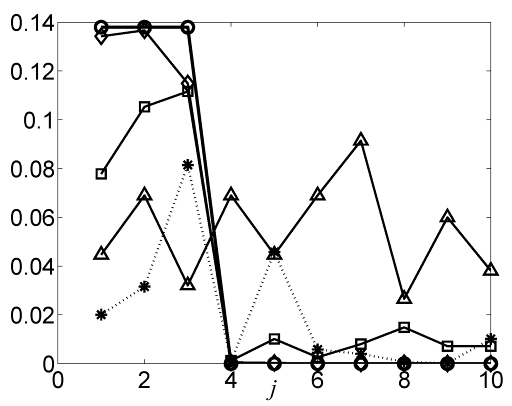
Figure 4.
The estimated for OR BNs with 10 variables, where on different datasets. The unit is a bit. The curve marked with circles is learned from the truth table of , so it is the ideal case, or the Golden Rule. The curves marked with diamonds, squares, triangles and stars represent the values obtained from truth table of , datasets of , , and with 10% noise, respectively.
In a binary system, there are only two values for variables. If we replace the zero in the OR BN truth table with one and vice versa, the resulting BN has opposite probabilities of one and zero to those of the original OR BN, respectively. It is easy to show that such a BN is an AND BN defined in the following.
Definition 4
The AND BN of a set of binary variables is, :
where the “∧” is the logical AND operation.
From Theorem 14, it is straightforward to obtain the following corollary.
Definition 4
For sufficiently large , if the samples are noiseless and randomly generated from a uniform distribution, then the DFL algorithm can identify an AND BN with an indegree of k in time, strictly.
Similarly to generalized OR BN, we define generalized AND BN in the following and obtain Corollary 5.
Definition 5
The generalized AND BN of a set of binary variables is, :
where the “∧” is the logical AND operation; can also take their inverted values.
Corollary 5
For sufficiently large , if the samples are noiseless and randomly generated from a uniform distribution, then the DFL algorithm can identify a generalized AND BN with an indegree of k in time, strictly.
4.3. The Complexity Analysis For Unbounded OR BNs
From Theorem 14, we see that the complexity of the DFL algorithm is if k becomes n.
However, according to Theorem 9, it needs samples to successfully find the BN of indegree n. In other words, an exponential number of samples makes the complexity of the DFL algorithm very high in this case, even if enough samples are provided. Therefore, it remains an open problem whether there are efficient algorithms for inferring AND/OR functions with unbounded indegrees, as proposed by Akutsu et al. [8].
However, if the indegree of the OR/AND BN is undetermined, but known to be much smaller than n, the DFL algorithm is still efficient. Biological knowledge supports this situation, because in real gene regulatory networks, each gene is regulated by a limited number of other genes [42]. In these cases, the expected cardinality, k, can be assigned as n, and the DFL algorithm can automatically find how many variables are sufficient for each . From Theorem 14, the DFL algorithm still has the complexity of for the OR/AND BN, given enough samples.
5. Results
We implement the DFL algorithm with the Java programming language (version 1.6). The implementation software, called DFLearner, is available for non-commercial purposes upon request.
In this section, we first introduce the synthetic datasets of BN models that we use. Then, we perform experiments on various data sets to validate the efficiency of the DFL algorithm. In the following, we carry out experiments on small datasets to examine the sensitivity of the DFL algorithm. The sensitivity is the correctly identified true input variables divided by the total number of true input variables [40]. Additionally, the specificity is the identified true non-input variables divided by the total number of non-input variables. We next compare the DFL algorithm with two existing methods in the literature under the same settings. The performance of the DFL algorithm on noisy datasets was also evaluated in our early work [40].
5.1. Synthetic Datasets of BNs
We present the synthetic datasets of BNs in this section. For a BN consisting of n genes, the total state space is . The v of a transition pair is randomly chosen from possible instances of V with the Discrete Uniform Distribution, i.e., , where i is a randomly chosen value from zero to , inclusively. Since the DFL algorithm examines different subsets in the kth layer with lexicographic order (see Figure 1), the run time of the DFL algorithm may be affected by the different positions of the target subsets in the kth layer. Therefore, we select the first and the last k variables in V as the inputs for all . The datasets generated from the first k and last k variables are named “head” and “tail” datasets. If the k inputs are randomly chosen from the n inputs, the datasets are named “random” datasets. There are different Boolean functions when the indegree is k. Then, we use the OR function (OR), the AND function (AND) or one of the Boolean functions randomly selected from possible functions (RANDOM) to generate the , i.e., . If two datasets are generated by the OR functions defined with the first and last k variables, then we name them OR-head and OR-tail datasets (briefly as OR-h and OR-t), respectively, and so on. Additionally, the Boolean function used to generate a dataset is called the generating Boolean function or, briefly, the generating function, of the dataset. The noisy samples are generated by reversing their output values. The program used to generate our synthetic datasets has been implemented in the Java programming language and been included in the DFLearner package.
5.2. Experiments for Time Complexities
As introduced in Theorem 14, the complexity of the DFL algorithm is for the OR/AND BNs given enough noiseless random samples from the uniform distribution. We first perform experiments for the OR/AND BNs to further validate our analysis. Then, we perform experiments for the general BNs to examine the complexity of the DFL algorithm for them.
5.2.1. Complexities for Bounded OR/AND BNs
In all experiments in this section, the training datasets are noiseless and the expected cardinality, k, and ϵ of the DFL algorithm are set to k of the generating functions and zero, respectively. In this study, we perform three types of experiments to investigate the effects of k, n and N in , respectively. In each type of experiment, we change only one of k, n or N and keep the other two unchanged. We generate 20 OR and 20 AND datasets for each k, N and n, respectively, i.e., 10 OR-h, 10 OR-t, 10 AND-h and 10 AND-t datasets. Then, we use the average value of these 20 datasets as the run time for this k, N and n value, respectively.
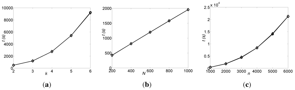
Figure 5.
The run times, t (vertical axes, shown in seconds), of the DFL algorithm for inferring the bounded Boolean networks (BNs). The values shown are the average of 20 noiseless datasets. The curves marked with circles and diamonds are for OR and AND datasets, respectively. (a) The run time vs. k, when n = 1000 and N = 600; (b) The run time vs. N, when n = 1000 and k = 3; (c) The run time vs. n, when k = 3 and N = 200.
First, we perform the experiments for various k, when n = 1000 and N = 600. The run times are shown in Figure 5a. Then, we perform the experiments for various N, when n = 1000 and k = 3. The run times of these experiments are shown in Figure 5b. Finally, we perform the experiments for various n, when k = 3 and N = 200. The run times are shown in Figure 5c. In all experiments for various k, N and n, the DFL algorithm successfully finds the original BNs.
As shown in Figure 5, the DFL algorithm uses almost the same times to learn the OR and AND BNs. As introduced in Theorem 14 and Corollary 4, the DFL algorithm has the same complexity of for learning the OR and AND BNs. The run time of the DFL algorithm grows slightly faster than linear with k, as shown in Figure 5a. This is due to the fact that the computation of entropy and MI takes more time when k increases. As shown in Figure 5b, the run time of the DFL algorithm grows linearly with N. Additionally, as in Figure 5c, the run time of the DFL algorithm grows quasi-squarely with n. A BN with 6,000 genes can correctly be found in a modest number of hours.
5.2.2. Complexities for Unbounded OR/AND BNs
To examine the complexity of the DFL algorithm for the unbounded OR/AND BN, we generate 20 OR datasets (10 OR-h and 10 OR-t) with N = 10, 000, n = 10, and the k is chosen from two to 10. Then, we apply the DFL algorithm to these datasets. In all experiments of this section, the expected cardinality, k, and ϵ of the DFL algorithm are set to 10 and zero, respectively, since it is assumed that the DFL algorithm does not know the indegrees of BNs a priori.
The DFL algorithm successfully finds the original BNs for all data sets. The average run times of the DFL algorithm for these data sets are shown in Figure 6a. The numbers of the subsets checked by the DFL algorithm for learning one OR Boolean function are shown in Figure 6b. As shown in Figure 6a, the run time of the DFL algorithm grows linearly with k for the unbounded OR datasets. In Figure 6b, the number of subsets checked by the DFL algorithm is exactly for the unbounded OR datasets. In other words, the complexity of the DFL algorithm is in the worst case for learning the unbounded OR BNs given enough samples. The DFL algorithm checks slightly more subsets for the OR-t data sets than for the OR-h datasets, when k < 10. This is due to the fact that the DFL algorithm examines different subsets in the kth layer with lexicographic order.
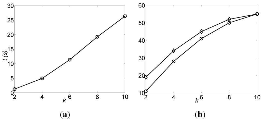
Figure 6.
The efficiency of the DFL algorithm for the unbounded OR datasets. The values shown are the average of 20 OR noiseless datasets. (a) The run time, t (vertical axis, shown in seconds), of the DFL algorithm to infer the unbounded BNs; (b) The number of the subsets checked by the DFL algorithm for learning one OR Boolean function. The curves marked with circles and diamonds are for OR-h and OR-t datasets, respectively.
5.2.3. Complexities for General BNs
In all experiments in this section, the expected cardinality, k, and ϵ of the DFL algorithm are set to k of the generating functions and zero, respectively. To examine the complexity of the DFL algorithm for general BNs, we examine the BNs of k = 2, k = 3 and n = 100. There are and possible Boolean functions whose output values correspond to binary 0 to binary 15 and 255, respectively. We use the decimal value of the output value of a Boolean function as its index. For instance, the index of the OR function of k = 2 is seven, since its output value is 0111, i.e., decimal 7. Thus, we generate 16 and 256 BNs, which are determined by the 16 and 256 Boolean functions when k = 2 and k = 3, respectively. For each BN, we generate the noiseless “head”, “random” and “tail” data sets, and the average run times of five independent experiments of these three datasets are shown in Figure 7.
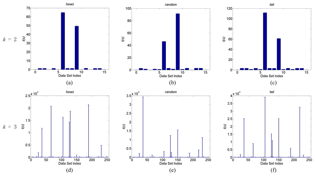
Figure 7.
The run times of the DFL algorithm for learning general BNs. (a) to (c) are run times on noiseless head, random and tail datasets of k = 2, respectively; (d) to (f) are run times on noiseless head, random and tail datasets of k = 3, respectively. The horizontal axes are the index of datasets and vertical axes are the run times, t, in seconds. The average sensitivities of the DFL algorithm are 100% for datasets of Part (a) to (c), and over 99.3% for datasets of Part (d) to (f). The shown times are the average values of five runs. The error bars are the standard deviations. These experiments were performed on a computer with an Intel Xeon 64-bit CPU of 2.66 GHz and 32 GB memory running the CENTOS Linux operating system.
In Figure 7a–c, it is clear that all BNs of k = 2 can be learned in a few seconds, except the two with index 6 and 9. We find that their corresponding generating Boolean functions are exclusive OR ⨁ and Boolean equality ≡, respectively, as shown in Table 5. In all experiments in Figure 7a–c, the DFL algorithm successfully identifies the original generating functions of data sets, i.e., achieving sensitivities of 100%. According to Figure 7d–f, we also check the ten BNs that the DFL algorithm uses more time to learn and list their generating functions in Table 5. In all of these BNs, the input variables of their generating Boolean functions are related with ⨁ or ≡ and their combinations. The average sensitivities of the DFL algorithm are over 99.3% for experiments in Figure 7d–f. We then examine the number of subsets that are searched when the DFL algorithm finds the target subsets. Except the ten BNs with generating functions listed in Table 5, the DFL algorithm only checks subsets before finding the true input variable subsets for each . As to be discussed in the following sections, only 218 out of 256 BNs of k = 3 actually have three inputs. Therefore, when the datasets are noiseless, the DFL algorithm can efficiently learn most, > 95% (208/218), general BNs of k = 3 with the time complexity of with a very high sensitivity of over 99.3%.
Table 5.
The generating Boolean functions of BNs that the DFL algorithm used more computational time to learn.
| Index | Generating Boolean Function |
|---|---|
| k = 2 | |
| 6 | |
| 9 | |
| k = 3 | |
| 24 | |
| 36 | |
| 66 | |
| 105 | |
| 126 | |
| 129 | |
| 150 | |
| 189 | |
| 219 | |
| 231 |
5.3. Experiments of Small Datasets
From Theorem 9, it is known that the sufficient sample size for inferring BNs is related to the indegree, k, and the number of variables, n, in the networks. Therefore, we apply the DFL algorithm to 200 noiseless OR (100 OR-h and 100 OR-t) and 200 noiseless RANDOM (100 RANDOM-h and 100 RANDOM-t) datasets with k = 3, n = 100 and various N. Then, we apply the DFL algorithm to 200 noiseless OR (100 OR-h and 100 OR-t) datasets, where k = 3, n = 100, 500, 1000 and various N. Finally, we apply the DFL algorithm to 200 noiseless OR (100 OR-h and 100 OR-t) datasets, where k = 2, 3, 4, n = 100 and various N. The relation between the sensitivity of the DFL algorithm and N is shown in Figure 8. In all experiments in this section, the expected cardinality, k, and ϵ of the DFL algorithm are set to k of the generating functions and zero, respectively.
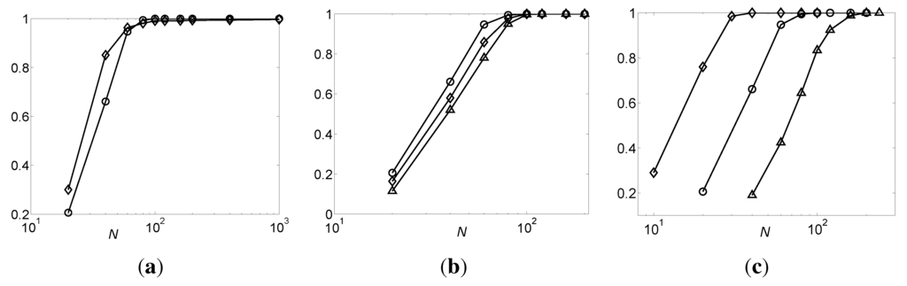
Figure 8.
The sensitivity of the DFL algorithm vs. sample size N. The values shown are the average of 200 noiseless datasets. (a) The sensitivity vs. N for OR and RANDOM datasets, when n = 100, k = 3. The curves marked with circles and diamonds are for OR and RANDOM datasets, respectively; (b) The sensitivity vs. N for OR datasets, when n = 100, 500, 1000, and k = 3. The curves marked with circles, diamonds and triangles are for data sets of n = 100, 500 and 1000, respectively; (c) The sensitivity vs. N for OR datasets, when k = 2, 3, 4, and n = 100. The curves marked with diamonds, circles and triangles are for data sets of k = 2, 3 and 4, respectively.
From Figure 8, it is shown that the sensitivity of the DFL algorithm grows approximately linearly with the logarithmic value of N, but becomes one after a certain N value, except the RANDOM datasets in part (a). For the RANDOM datasets, the sensitivity of the DFL algorithm has increased to 99.3% when N = 200 and, further, to 99.7% when N = 1000. This means that if the training dataset is large enough, the DFL algorithm can correctly identify the original OR BNs and correctly find the original RANDOM BNs with a very high probability.
As shown in Figure 8b, for the same N ∈ (0, 100), the sensitivity of the DFL algorithm shows a small decrease when n increases. Figure 8c shows that, for the same N, the sensitivity shows a large decrease when k increases. This is due to the different effect of k and n in determining the sufficient sample size. In Theorem 9, the sufficient sample size, N, grows exponentially with k, but linearly with log n. However, in both Figure 8b and c, the sensitivity of the DFL algorithm gradually converges to 100% when N increases.
We also find that when the sample size is small, the DFL algorithm may use more time than . For example, the average run times of the DFL algorithm for the 200 small OR datasets of n = 100 and k = 3 used in this section are shown in Figure 9. The complexity of the DFL algorithm is bad when the sample size N falls into the region from 20 to 100, but resumes linear growth after N is bigger than 100.

Figure 9.
The run time, t (vertical axis, shown in seconds), of the DFL algorithm for small OR datasets, where n = 100 and k = 3. The values shown are average of 200 datasets.
5.4. Comparisons with Existing Methods
Maucher et al. [16] presented a comparison of their correlation algorithm and the best fit algorithm [19,20] on 50 random BNs with monotonic generating functions [16]. We generate datasets using the same settings of [16], except the generating functions. In contrast to only monotonic generating functions used in [16], we generate the same number of samples, from 50 to 800, with 10% noise for all BNs of k = 3, with n = 10 and 80, respectively. In the 256 Boolean functions of k = 3, there are 38 functions whose numbers of input variables are actually less than 3. Among Boolean functions of k = 2, there are two constant functions and four functions with only one input. Thus, only 10 BNs really have two inputs among 16 BNs of k = 2. Hence, there are 30 functions with two inputs, six functions with one input and two constant functions among the 256 Boolean functions of k = 3. Only the remaining 218 BNs with three inputs are used, because the other BNs represent models of k < 3. For each of the 218 BNs, we generate three datasets, one “head”, one “random” and one “tail”, for each sample size. Then, the average sensitivities and specificities for each sample size are calculated for the 218 “head”, 218 “random” and 218 “tail” datasets, respectively. Then, the results of “head”, “random” and “tail” datasets are combined to calculate the average values and standard deviations shown in Figure 10.
We use the ϵ-value method introduced in Methods to handle the noise issue. We try different ϵ-values from zero to one with a step of 0.01. Because there are no subsets that satisfy in noisy datasets, the DFL algorithm falls into the exhaustive search of subsets with ≤ k input variables. Thus, we use a restricted searching method that only checks subsets at each ϵ-value for the datasets of n = 80. In the restricted searching method, all subsets with one variable are examined, and the subset, say , with the largest MI with Y is kept. Then, the DFL algorithm continues to check n − 1 two element subsets with , and the subset with the largest MI with Y among these n − 1 subsets, say , is kept. This searching procedure continues, until k input variables are chosen.

Figure 10.
The performance of the DFL algorithm when learning general BNs from datasets of 10% noise with different sample sizes. For each sample size, three (one “head”, one “random” and one “tail”) datasets were generated for each of the 218 BNs of k = 3. The sensitivities, specificities and the number of data sets, m, on which the DFL algorithm successfully achieved 100% sensitivities and specificities were calculated on the 218 “head”, 218 “random” and 218 “tail” datasets, respectively. Then, the average values in the curves and standard deviations (the error bars) were calculated from the averages of the “head”, “random” and “tail” datasets. The curves marked with circles (blue), DFLr, and dots (red), DFLx, represent the average values on the datasets of n = 80 with restricted searching of only subsets and n = 10 with exhaustive searching of subsets, respectively. The curves marked with triangles (green), best-fit, and diamonds (magenta), Corr., are the average values of the Best-fit and Correlation algorithm on noisy datasets of 50 monotonic Boolean networks with n = 80 and Gaussian noise with SD σ = 0.4 (reported in [16]), respectively. (a) The sensitivities vs. N; (b) The specificities vs. N; (c) The number of datasets, m, on which the DFL algorithm achieved 100% sensitivities and specificities.
The exhaustive search is used for the datasets of n = 10. The BNs learned with the smallest ϵ-values are compared with the generating functions to calculate the sensitivities and specificities that are shown in Figure 10a and b. We calculate the numbers of BNs that are learned by the DFL algorithm with 100% sensitivities and specificities, as shown in Figure 10c. We also compare the results of the DFL algorithm in Figure 10 to those of two existing algorithms reported in [16] (in Figure 1 of [16]).
The DFL algorithm using exhaustive search achieves good sensitivities and specificities when N > 100 on datasets of n = 10, Figure 10a and b. In comparison with the Correlation algorithm [16], the DFL algorithm shows much better specificities and sensitivities, especially when N < 200. When compared with the Best-fit algorithm [12], the DFL algorithm demonstrates much better sensitivities when N < 200 and comparable specificities.
As shown in Figure 10, the performance of the DFL algorithm using restricted searching decreases a little bit. When compared with the Best-fit algorithm, DFL using restricted searching has better sensitivities when N < 250, but has slightly worse specificities. DFL using restricted searching shows better specificities than the Correlation algorithm when N < 600, but has slightly worse sensitivities for N < 100. Remember that our datasets that are applied to the DFL algorithm also consist of non-monotonic functions, such as those listed in Table 5. When the restricted searching is used, it is possible that the DFL algorithm cannot correctly learn the original generating functions for these datasets whose . This explains why the DFL algorithm demonstrates a slightly declined performance when the restricted searching strategy is used. Recall that the results of the Best-fit and Correlation algorithm reported in [16] are obtained on datasets of 50 monotonic functions. Therefore, the performance of the DFL algorithm is still comparable to these two methods, even using the restricted searching method. It is also interesting to point out in Figure 10c that the DFL algorithm can successfully identify about 98% BNs using the exhaustive searching and can soundly learn about 185 (85%) BNs, even using the restricted searching when N < 200. In other words, when maintaining 100% sensitivity and specificity, the DFL algorithm keeps its complexity of for learning these 85% BNs of k = 3 from noisy datasets.
In summary, these results demonstrate that the DFL algorithm has a better comprehensive performance than the methods compared in this study.
6. Discussion
6.1. Advantages of the DFL Algorithm
An advantage of the DFL algorithm is that it requires less samples to achieve good sensitivities and specificities than existing methods. As shown in Figure 10, when the sample size is larger than 100, the DFL algorithm achieves over 98% sensitivities and specificities using exhaustive searching. Taking the log n in Theorem 9 into consideration, the DFL algorithm needs around 200 samples to achieve over 98% sensitivities for learning BNs of n = 80. As demonstrated in Figure 10, the DFL algorithm achieves sensitivities of about 90% and specificities of about 95% when N ≥ 200 when the restricted searching is used, i.e., only using time. When compared with the DFL algorithm using the restricted searching, the results in [16] show that the Best-fit algorithm [12] needs more samples to achieve comparable sensitivity of 90%, and its time complexity is , which is much worse than of the DFL algorithm. The Correlation algorithm demonstrates similar sensitivity to the DFL algorithm when N ≥ 200, but its specificities are much worse than those of the DFL algorithm, with a value of about 78% when N = 200. Another advantage of the DFL algorithm is that it can learn more general BNs than the Correlation algorithm [16], as shown in Figure 7 and Figure 10. Actually, the DFL algorithm can successfully learn 208 and 185 BNs of the 218 (about 95% and 85%, respectively) BNs of k = 3 from noiseless and noisy datasets, respectively, only using the time; Figure 7d–f and Figure 10c. Furthermore, if the computation time is less important than sensitivities and specificities, the DFL algorithm can achieve better performance for noisy datasets by using the exhaustive searching strategy, as shown in Figure 10, for other BNs.
6.2. The Noise and Size of Training Datasets
Let us consider the factors that affect the sensitivity of the DFL algorithm. As shown in Figure 4, the of BNs is affected by two factors, the sample size, N, and the noise levels of datasets.
One factor that affects the complexity of the DFL algorithm is the amount of noise in the training datasets. This is because noise changes the distributions of X and Y, thus destroying the equality between and if . Therefore, we use the ϵ-value method to learn BNs from noisy datasets [21,37,40]. As shown in Figure 10, the DFL algorithm achieves > 99% sensitivities and specificities when N > 100, if the exhaustive searching strategy is used. The DFL algorithm can successfully identify most general BNs from noisy datasets, around 98%(213/218), given enough samples, as shown in Figure 10c. The results in Figure 10a and Figure 8a show that the performance of the DFL algorithm is stable for noisy data sets, even when the percentage of the noise samples is increased to 20% [40]. To keep its efficiency, a restricted searching method is also examined in Figure 10 for the datasets of n = 80. Our results demonstrate that most BNs, about 85%, can be learned very efficiently with the restricted searching method in a time complexity of . Thus, it is advantageous to use the restricted searching to find a model and to refine it with exhaustive searching when using the DFL algorithm in practice.
In addition to the level of noise, sample size is another factor that affects the time complexity of the DFL algorithm. As demonstrated in Figure 8, the DFL algorithm shows increasing sensitivities when the sample sizes increases, and the sensitivity of the DFL algorithm converges to 100% when enough samples are provided. In the meantime, in Figure 9, the running time shows an interesting convex pattern when the sample size is small, but increases linearly when the number of samples reaches a threshold. That is because the DFL algorithm is disturbed by other irrelevant variables when the sample size is small. Let us use the example in Figure 4 to explain the issue. In the ideal case, or the Golden Rule, , , should be values generated from the truth table of the generating function, and , , based on Theorem 8. In this example, tends to be zero given enough samples. Actually, when N = 1000, the for is almost zero, as shown in Figure 4. However, when N is small, the is very different. Many irrelevant variables have non-zero . Thus, it takes many additional computations to find the correct , which explains the increased computational time in Figure 9 when N is small. Even worse, there probably exist other subsets of V, which satisfy the criterion of Theorem 5. For instance, the DFL algorithm finds that , which is incorrect, since when N = 20 in the example of Figure 4. Consequently, it is possible that the DFL algorithm cannot find the original BNs. Theorem 10 is correct no matter how many learning samples are provided. In cases of small sample sizes, such as N = 20 in the example, the obtained BNs are still consistent with the learning datasets. However, the sensitivity of the DFL algorithm becomes 1/3 for this example, since only 1/3 of the edges of the original network are correctly identified. In this case, the consistency used by [5] is not suitable for evaluating the performance of a learning algorithm. This explains why we use the sensitivity to evaluate the performance of the DFL algorithm.
Recently, Perkins and Hallett [43] provided an improved sample complexity for learning BNs. They also demonstrated that uncorrelated samples reduce the number of samples needed, but increase the learning time, and strongly correlated samples have the opposite effect. Their findings suggest that the correlation between samples should also be considered when using DFL to learn BNs, depending on the preference of either less samples or less computational time.
Sample distribution is another point to be mentioned. Because Theorem 6 is correct regardless of sample distribution, the MI and entropy can be correctly estimated from enough samples randomly drawn from distributions other than the uniform distribution. Therefore, we hypothesize that Theorem 14 and Corollaries 3, 4 and 5 are also correct on the training samples drawn from other distributions, although this theorem and these corollaries require that the learning samples are randomly drawn from the Discrete Uniform Distribution.
6.3. The BNs With More Computation Time
In some Boolean functions, such as the ⨁ functions, for . This makes it very unlikely to rank the in the front part of the list after the sort step in line 7 of Table 3. Fortunately, in the empirical studies in Figure 7, the worst case happens with very low probability, < 5%, for inferring general BNs with an indegree of three. The experimental results show that although the DFL algorithm uses more steps for finding the target subsets for those functions whose than for other functions, its complexity is still polynomial for each .
In the context of GRNs, the exclusive OR and Boolean equality function are also unlikely to happen between different regulators of a gene. In some cases, a gene can be activated by several activators, and any of these activators is strong enough to activate the gene. This can be modeled as an “OR” logic between these activators. In other cases, several activators must simultaneously bind to their binding sites in the cis-regulatory region to turn on the gene, which can be modeled as an “AND” logic. A repressor often turns off the gene, so it can be modeled as the “INVERT” logic. Suppose that the regulators act with ⨁ relation; then, it needs an odd number of regulators with a high expression level (in the logic 1 state). For example, a gene, X, has one activator, A, and one repressor, R; then, . The second term on the right side says that if the activator is on its low level and the repressor is on its high level, then X will be turned on, which is clearly unreasonable. Similarly, suppose . The first term on the right side means that X will be turned on if both A and R are on their low levels. This situation is also unreasonable. From the above analysis, the exclusive OR and Boolean equality relations are unlikely to happen in a real biological system, which is also argued in [16].
6.4. The Constant Functions
The DFL algorithm outputs that “ is a constant” for two extreme cases, i.e., = 1 or 0, . Since, in these two cases, the is a constant, the entropy of is zero. In other words, the information content of is zero. Therefore, it is unnecessary to know which subset of features are the genuine inputs of in these two cases.
In case of GRNs, some genes show constant expression levels in a specific biological process. For example, a large amount of genes do not show significant changes in their expression levels during the yeast, Saccharomyces cerevisiae, cell-cycle in the study of [38]. These genes are considered as house-keeping genes and removed before further analysis of the expression datasets [38].
However, it is also possible that only one output value appears in the training samples, especially when the datasets are limited. In this case, the DFL algorithm still reports the model as a constant, which is not true. Thus, it is advisable to check the sample size based on Theorem 9 to make sure that the sample size is large enough if there is a possibility that the underlying generating function should not be a constant based on prior knowledge.
7. Conclusions
We prove that the DFL algorithm can learn the OR/AND BNs with the time complexity in the worst case given enough noiseless random samples drawn from the uniform distribution. The experimental results validate this conclusion. Our experiments demonstrate that the DFL algorithm can successfully learn > 95% BNs of k = 3 with the same complexity of from noiseless samples. For noisy datasets, the DFL algorithm successfully learns about 85% of BNs of k = 3 using the time. Furthermore, when the datasets are noisy, the DFL algorithm can successfully learn more BNs of k = 3, about 98%, using the exhaustive searching; Figure 10c.
Although the learning of Boolean functions is discussed in this paper, the DFL algorithm has also been demonstrated to learn multi-value discrete functions or GRN models. For example, we use the DFL algorithm to learn GLFmodels [44], in which genes are related with multi-value functions, in our early work [21,40].
Since Boolean function learning algorithms have been used to solve many problems [22,23,24,25,26,27,28,29,30], the DFL algorithm can potentially find its application in other fields, such as classification [41,45,46,47], feature selection [37], pattern recognition, functional dependencies retrieving and association rules retrieving.
Author’s Contributions
Yun Zheng and Chee Keong Kwoh conceived of and designed the research. Yun Zheng conducted the theoretical analysis, implemented the method and performed the experiments. Yun Zheng and Chee Keong Kwoh analyzed the results and wrote the manuscript. Both authors read and approved the final manuscript.
Acknowledgements
The research is supported in part by a grant of Jardine OneSolution (2001) Pte Ltd to Chee Keong Kwoh and a start-up grant of Kunming University of Science and Technology to Yun Zheng.
Conflicts of Interest
The authors declare no conflict of interest.
Appendix
Proofs of the Theorems
Theorem 15
([34](p. 33)) If , .
Theorem 8
If , and X and Z are independent, then: .
Proof 1
Since X and Z are independent, based on Theorem 1, we have:
Since , based on Theorem 5, we have . Then, based on Theorem 15, we have
From Equations (11) and (12), we have . Based on Theorem 1, we have .□
Theorem 11
In an OR BN with an indegree of k over V, the mutual information between and is:
Proof.
Without loss of generality, we consider . In the truth table of , there are equal numbers of “0” and “1” for . Thus, .
In the truth table of , there are lines totally. Additionally, in the column of , there is only one “0”, and “1”. Thus,
There are only three possible instances for the tuple, , i.e., (0, 0), (0, 1) and (1, 1). By counting the numbers of these instances, and divided by the total number of lines, we have
Therefore, we obtain
□
Theorem 12
In an OR BN with an indegree of k over V, , , the mutual information between and is
Proof.
Similar to the proof of Theorem 11, we have
Consider and p = 2 first. Without loss of generality, we derive . For , as shown in Table A1, there are possible instances for , i.e., (0,0), (0,1), (1,0) and (1,1). By counting the number of these instances and dividing by the total number of lines, we get (bits).
Table A1.
The truth table of .
| X1 | X2 | X3 | |
|---|---|---|---|
| 0 | 0 | 0 | 0 |
| 0 | 0 | 1 | 1 |
| 0 | 1 | 0 | 1 |
| 0 | 1 | 1 | 1 |
| 1 | 0 | 0 | 1 |
| 1 | 0 | 1 | 1 |
| 1 | 1 | 0 | 1 |
| 1 | 1 | 1 | 1 |
Next, we derive . There are possible instances for , i.e., (0,0,0), (0,0,1), (0,1,1), (1,0,1) and (1,1,1). Their probabilities are
Hence, we get
Finally, we have
By generalizing three to p, we have
From Equation (19), there is one instance of for . There are instances of for . There are possible instances of with the same probabilities of . Hence,
Finally, by combing Equations (18), (22) and (23), we have the result, ,
□
When , from Theorem 12, we have , as shown in Equation (18). This result is exactly consistent with Theorem 4, which validates Theorem 12 from another aspect. For instance, as shown in Figure 3b, when p = 6, the in the curve for k = 6 is 0.116 bits, which should be equal to from Theorem 4. Then, from Equation (18), when k = 6, bits, too.
Theorem 13
In an OR BN with an indegree of k over V, , .
Proof.
From Theorem 12, we have
Thus:
Since monotonically increases , so ; thus, , . Therefore, monotonically increases with p, . So, we have the result.□
The correctness of Theorem 13 is also demonstrated in Figure 3b.
Theorem 14
For sufficiently large , if the samples are noiseless and randomly generated from a uniform distribution, then the DFL algorithm can identify an OR BN with an indegree of k in time, strictly.
Proof.
The datasets are generated with the original Boolean functions of the BNs. From Theorem 6, the empirical probabilities of and in the Boolean functions, , tend to be the probabilities in the truth table of when the sample size is large enough.
First, consider the searching process in the first layer of the search graph, like Figure 1. From Theorem 8, we obtain if . Meanwhile, from Theorem 11, . Thus, s are listed in front of the other variables, Zs, after the sort step in line 7 of Table 3.
In the following, the (subsets with and another variable) are dynamically added to the second layer of the ΔTree. Now, consider the MI, , where Z is one of the variables in . First, if , from Theorem 8, . Since , and are independent variables, from Theorem 2, we get . From Theorem 3, we have:
Second, if , from Theorem 13, we have
After combining the results in Equations (28) and (29), we have that , is larger than the same measure when .
Therefore, in the second layer of the ΔTree, the combinations with two elements from are listed in front of other combinations, and so on so forth, until the DFL algorithm finds in the kth layer of the ΔTree, finally.
In the searching process, only subsets are visited by the DFL algorithm. Therefore, the complexity of the DFL algorithm becomes , where log n is for sort step in line 7 of Table 3 and N is for the length of input table T.□
Corollary 3
For sufficiently large , if the samples are noiseless and randomly generated from a uniform distribution, then the DFL algorithm can identify a generalized OR BN with an indegree of k in time, strictly.
Proof.
We replace those s that are taking their inverted values with another variable, , i.e., let ; then, the resulting BN is an OR BN. does not change in the new OR BN.
To satisfy the criterion of Theorem 5, compare the MI, , with . We have
remains the same value as the corresponding item in . In binary systems, there are only two states, i.e., “0” and “1”. It is straightforward to obtain . Therefore, the only item changed in the is the joint entropy, . Next, we prove that .
Consider the tuple, . If we replace “0’ of with “1” and vice versa, it becomes , as shown in Table A2. The three instances, (0, 0), (0, 1) and (1, 1), of change to (1, 0), (1, 1) and (0, 1) of , respectively. However, the probabilities (frequencies) of them are coincidentally equal, respectively. Thus, .
Table A2.
The tuple and , where k is two.
| 0 | 0 | 1 | 0 |
| 0 | 1 | 1 | 1 |
| 1 | 1 | 0 | 1 |
| 1 | 1 | 0 | 1 |
From Theorem 14, the results are obtained.□
Corollary 4
For sufficiently large , if the samples are noiseless and randomly generated from a uniform distribution, then the DFL algorithm can identify an AND BN with an indegree of k in time, strictly.
Proof.
In an AND BN, and are equal to and in a corresponding OR BN with the same for all , respectively. Therefore, is the same as that of the corresponding OR BN. From Theorem 14, the result can be directly obtained.□
Corollary 5
For sufficiently large , if the samples are noiseless and randomly generated from a uniform distribution, then the DFL algorithm can identify a generalized AND BN with an indegree of k in time, strictly.
Proof.
Similar to that of Corollary 3.□
References
- Davidson, E.; Levin, M. Gene regulatory networks special feature: Gene regulatory networks. Proc. Natl. Acad. Sci. USA 2005, 102. [Google Scholar] [CrossRef] [PubMed]
- Davidson, E.; McClay, D.; Hood, L. Regulatory gene networks and the properties of the developmental process. Proc. Natl. Acad. Sci. USA 2003, 100, 1475–1480. [Google Scholar] [CrossRef] [PubMed]
- Levine, M.; Davidson, E. From the cover. Gene regulatory networks special feature: Gene regulatory networks for development. Proc. Natl. Acad. Sci. USA 2005, 102, 4936–4942. [Google Scholar] [CrossRef] [PubMed]
- Kauffman, S. Metabolic stability and epigenesis in randomly constructed genetic nets. J. Theor. Biol. 1969, 22, 437–467. [Google Scholar] [CrossRef]
- Akutsu, T.; Miyano, S.; Kuhara, S. Identification of Genetic Networks from a Small Number of Gene Expression Patterns under the Boolean Network Model. In Proceedings of Pacific Symposium on Biocomputing ’99, Big Island, HI, USA, 4–9 January 1999; Volume 4, pp. 17–28.
- Akutsu, T.; Miyano, S.; Kuhara, S. Algorithm for identifying boolean networks and related biological networks based on matrix multiplication and fingerprint function. J. Comput. Biol. 2000, 7, 331–343. [Google Scholar] [CrossRef] [PubMed]
- Akutsu, T.; Miyano, S.; Kuhara, S. Inferring qualitative relations in genetic networks and metabolic pathways. Bioinformatics 2000, 16, 727–734. [Google Scholar] [CrossRef] [PubMed]
- Akutsu, T.; Miyano, S.; Kuhara, S. A simple greedy algorithm for finding functional relations: Efficient implementation and average case analysis. Theor. Comput. Sci. 2003, 292, 481–495. [Google Scholar] [CrossRef]
- Ideker, T.; Thorsson, V.; Karp, R. Discovery of Regulatory Interactions Through Perturbation: Inference and Experimental Design. In Proceedings of Pacific Symposium on Biocomputing, Island of Oahu, HI, USA, 4–9 January 2000; Volume 5, pp. 302–313.
- Kim, H.; Lee, J.K.; Park, T. Boolean networks using the chi-square test for inferring large-scale gene regulatory networks. BMC Bioinforma. 2007, 8. [Google Scholar] [CrossRef]
- Laubenbacher, R.; Stigler, B. A computational algebra approach to the reverse engineering of gene regulatory networks. J. Theor. Biol. 2004, 229, 523–537. [Google Scholar] [CrossRef] [PubMed]
- Lähdesmäki, H.; Shmulevich, I.; Yli-Harja, O. On learning gene regulatory networks under the boolean network model. Mach. Learn. 2003, 52, 147–167. [Google Scholar]
- Liang, S.; Fuhrman, S.; Somogyi, R. REVEAL, a General Reverse Engineering Algorithms for Genetic Network Architectures. In Proceedings of Pacific Symposium on Biocomputing ’98, Maui, HI, USA, 4–9 January 1998; Volume 3, pp. 18–29.
- Maki, Y.; Tominaga, D.; Okamoto, M.; Watanabe, S.; Eguchi, Y. Development of a System for the Inference of Large Scale Genetic Networks. In Proceedings of Pacific Symposium on Biocomputing, Big Island, HI, USA, 3–7 January 2001; Volume 6, pp. 446–458.
- Müssel, C.; Hopfensitz, M.; Kestler, H.A. BoolNet-an R package for generation, reconstruction and analysis of Boolean networks. Bioinformatics 2010, 26, 1378–1380. [Google Scholar] [CrossRef] [PubMed]
- Maucher, M.; Kracher, B.; Kühl, M.; Kestler, H.A. Inferring Boolean network structure via correlation. Bioinformatics 2011, 27, 1529–1536. [Google Scholar] [CrossRef] [PubMed]
- Maucher, M.; Kracht, D.V.; Schober, S.; Bossert, M.; Kestler, H.A. Inferring Boolean functions via higher-order correlations. Comput. Stat. 2012. [Google Scholar] [CrossRef]
- Nam, D.; Seo, S.; Kim, S. An efficient top-down search algorithm for learning boolean networks of gene expression. Mach. Learn. 2006, 65, 229–245. [Google Scholar] [CrossRef]
- Shmulevich, I.; Saarinen, A.; Yli-Harja, O.; Astola, J. Inference of genetic regulatory networks via best-fit extensions. In Computational and Statistical Approaches to Genomics; Zhang, W., Shmulevich, I., Eds.; Springer: New York, NY, USA, 2003; Chapter 11; pp. 197–210. [Google Scholar]
- Shmulevich, I.; Yli-Harja, O.; Astola, J.; Core, C.G. Inference of Genetic Regulatory Networks Under the Best-Fit Extension Paradigm. In Proceedings of the IEEE—EURASIP Workshop on Nonlinear Signal and Image Processing (NSIP-01), Baltimore, MD, USA, 3–6 June 2001; Kluwer Academic Publishers: Norwell, MA, USA, 2002; pp. 3–6. [Google Scholar]
- Zheng, Y.; Kwoh, C.K. Dynamic Algorithm for Inferring Qualitative Models of Gene Regulatory Networks. In Proceedings of the 3rd Computational Systems Bioinformatics Conference, CSB 2004, Stanford, CA, USA, 16–19 August 2004; IEEE Computer Society Press: Stanford, CA, USA, 2004; pp. 353–362. [Google Scholar]
- Birkendorf, A.; Dichterman, E.; Jackson, J.; Klasner, N.; Simon, H.U. On restricted-focus-of-attention learnability of boolean functions. Mach. Learn. 1998, 30, 89–123. [Google Scholar] [CrossRef]
- Bshouty, N.H. Exact learning Boolean functions via the monotone theory. Inf. Comput. 1995, 123, 146–153. [Google Scholar] [CrossRef]
- Eiter, T.; Ibaraki, T.; Makino, K. Decision lists and related Boolean functions. Theor. Comput. Sci. 2002, 270, 493–524. [Google Scholar] [CrossRef]
- Huhtala, Y.; Kärkkäinen, J.; Porkka, P.; Toivonen, H. TANE: An efficient algorithm for discovering functional and approximate dependencies. Comput. J. 1999, 42, 100–111. [Google Scholar] [CrossRef]
- Littlestone, N. Learning quickly when irrelevant attributes abound: A new linear-threshold algorithm. Mach. Learn. 1988, 2, 285–318. [Google Scholar] [CrossRef]
- Mannila, H.; Raiha, K. On the complexity of inferring functional dependencies. Discret. Appl. Math. 1992, 40, 237–243. [Google Scholar] [CrossRef]
- Mannila, H.; Räihä, K.J. Algorithms for inferring functional dependencies from relations. Data Knowl. Eng. 1994, 12, 83–99. [Google Scholar] [CrossRef]
- Mehta, D.; Raghavan, V. Decision tree approximations of Boolean functions. Theor. Comput. Sci. 2002, 270, 609–623. [Google Scholar] [CrossRef]
- Rivest, R.L. Learning decision lists. Mach. Learn. 1987, 2, 229–246. [Google Scholar] [CrossRef]
- Mossel, E.; O’Donnell, R.; Servedio, R.A. Learning functions of k relevant variables. J. Comput. Syst. Sci. 2004, 69, 421–434. [Google Scholar] [CrossRef]
- Arpe, J.; Reischuk, R. Learning juntas in the presence of noise. Theor. Comput. Sci. 2007, 384, 2–21. [Google Scholar] [CrossRef]
- Shannon, C.; Weaver, W. The Mathematical Theory of Communication; University of Illinois Press: Urbana, IL, USA, 1963. [Google Scholar]
- Cover, T.M.; Thomas, J.A. Elements of Information Theory; Wiley: New York, NY, USA, 1991. [Google Scholar]
- Pearl, J. Probabilistic Reasoning in Intelligent Systems: Networks of Plausible Inference; Morgan Kaufmann: San Mateo, CA, USA, 1988. [Google Scholar]
- Gray, R.M. Entropy and Information Theory; Springer: New York, NY, USA, 1991. [Google Scholar]
- Zheng, Y.; Kwoh, C.K. A feature subset selection method based on high-dimensional mutual information. Entropy 2011, 13, 860–901. [Google Scholar] [CrossRef]
- Spellman, P.; Sherlock, G.; Zhang, M.; Iyer, V.; Anders, K.; Eisen, M.; Brown, P.; Botstein, D.; Futcher, B. Comprehensive identification of cell cycle-regulated genes of the yeast Saccharomyces cerevisiae by microarray hybridization. Mol. Biol. Cell 1998, 9, 3273–3297. [Google Scholar] [CrossRef] [PubMed]
- Trapnell, C.; Williams, B.; Pertea, G.; Mortazavi, A.; Kwan, G.; van Baren, M.; Salzberg, S.; Wold, B.; Pachter, L. Transcript assembly and quantification by RNA-Seq reveals unannotated transcripts and isoform switching during cell differentiation. Nat. Biotechnol. 2010, 28, 511–515. [Google Scholar] [CrossRef] [PubMed]
- Zheng, Y.; Kwoh, C.K. Dynamic algorithm for inferring qualitative models of gene regulatory networks. Int. J. Data Min. Bioinforma. 2006, 1, 111–137. [Google Scholar] [CrossRef]
- Zheng, Y.; Kwoh, C.K. Identifying Simple Discriminatory Gene Vectors with An Information Theory Approach. In Proceedings of the 4th Computational Systems Bioinformatics Conference, CSB 2005, Stanford, CA, USA, 8–11 August 2005; pp. 12–23.
- Arnone, M.; Davidson, E. The hardwiring of development: Organization and function of genomic regulatory systems. Development 1997, 124, 1851–1864. [Google Scholar] [PubMed]
- Perkins, T.J.; Hallett, M.T. A trade-off between sample complexity and computational complexity in learning boolean networks from time-series data. IEEE/ACM Trans. Comput. Biol. Bioinforma. 2010, 7, 118–125. [Google Scholar] [CrossRef] [PubMed]
- Thomas, R.; d’Ari, R. Biological Feedback; CRC Press: Boca Raton, FL, USA, 1990. [Google Scholar]
- Zheng, Y.; Hsu, W.; Lee, M.L.; Wong, L. Exploring Essential Attributes for Detecting MicroRNA Precursors from Background Sequences. In Data Mining and Bioinformatics; Revised Selected Papers of First International Workshop, VDMB 2006, Seoul, Korea, 11 September 2006; Dalkilic, M.M., Kim, S., Yang, J., Eds.; Volume 4316, Lecture Notes in Computer Science; Springer: Berlin/Heidelberg, Germany, 2006; pp. 131–145. [Google Scholar]
- Zheng, Y.; Kwoh, C.K. Cancer classification with MicroRNA expression patterns found by an information theory approach. J. Comput. 2006, 1, 30–39. [Google Scholar] [CrossRef]
- Zheng, Y.; Kwoh, C.K. Informative MicroRNA Expression Patterns for Cancer Classification. In Data Mining for Biomedical Applications, Proceedings of PAKDD 2006 Workshop, BioDM 2006, Singapore, Singapore, 9 April 2006; Li, J., Yang, Q., Tan, A.-H., Eds.; Volume 3916, Lecture Notes in Computer Science. Springer: New York, NY, USA, 2006; pp. 143–154. [Google Scholar]
© 2013 by the authors; licensee MDPI, Basel, Switzerland. This article is an open access article distributed under the terms and conditions of the Creative Commons Attribution license (http://creativecommons.org/licenses/by/3.0/).