1. Introduction
The possible existence of a time operator in Quantum Mechanics has long been a subject of interest. This subject has been studied from different points of view and has led to several developments in quantum theory. At the end of this paper there is a short, incomplete, list of papers on this subject.
However, we can also study the time variable in classical systems to begin to understand how to address time in quantum systems. In fact, we find that many of the difficulties encountered when addressing the time variable in quantum systems are also found in classical systems.
However, we usually only know a dynamical quantity with certainty whereas the conjugate quantity is not well known. This is the case for the pair of conjugate variables energy and time. In this paper, we introduce a method of generating an unknown coordinate related to a conjugate pair of dynamical variables F and G, which may be classical or quantum. This is particularly important in quantum systems because this is related to the understanding of time in quantum mechanics. There are no clear methods to define time states, but in this paper, we provide a way to generate these states.
In
Section 2, we discuss conjugate variables, introducing the related four vector fields that can generate the motion of points and of functions in phase space along different directions.
In
Section 3, we introduce a method for generating a coordinate system for a conjugate pair of dynamical variables, including the best choice for the zero time curve. We illustrate the procedure with three examples: the free particle, the harmonic oscillator, and a nonlinear oscillator.
In
Section 4, we generate a time coordinate for quantum systems with discrete spectra. There are some concluding remarks at the end of this paper.
Our point of view is that the conjugate variables F and G can be used to define an alternative coordinate system in phase space for classical systems or alternative representations for quantum systems.
2. Conjugate Variables
Let us consider a classical system and two conjugate functions
and
, where
,
, is a point in phase space. The conjugacy condition,
(the Poisson bracket between the variables), can be expressed in several ways:
where
and
The two vector fields
and
can be used to generate the motion of points and functions in phase space in two conjugate directions: along the
F or the
G direction. The vectors
and
form a basis of a symplectic vector space of dimension two, under the skew-symmetric map
, with rank two [
1].
Under the standard symplectic form
, the vector fields
and
comply with the fundamental relation, with different signs:
Hereafter, we will use dimensionless units with appropriate scaling parameters. Note that the Poisson bracket between the same dynamical variable vanishes. When applied to the
G variable, this fact may be expressed as follows:
This equality defines a vector field
that is normal to the constant
G shell. The vector field normal to the constant
F shell is
. Thus, the pair of vectors
and
or
and
are orthogonal. We will take advantage of these properties to choose the initial time eigenstate.
We have found four vector fields indicating four directions along which we can move functions or phase-space points. The dynamical system defined by the vector field
(when
is the Hamiltonian of a physical system),
has been of interest because this system describes the time evolution of phase-space points when
G is the Hamiltonian of a physical system. However, the other vector fields
,
, and
generate other types of symplectic and non-symplectic motions of points in phase-space:
which are also useful, as we will see below, in the examples. Here,
f and
g are used for parametrization of the trajectories of the points. They have the same units as
F and
G respectively. When
G is a Hamiltonian of a physical system,
f correspond to the time variable.
As we observed in Equation (
1),
and
G, as well as
and
F, are conjugate pairs. Therefore,
and
can be used to translate functions in phase space along the
G or
F directions as follows: [
2,
3,
4]
The derivatives of these functions are
We recognise the last equation, when
G is the Hamiltonian of a physical system, as the Liouville equation of motion. Note that, at the sites in which
vanishes, the dynamical system generated by
G moves points only along the position axis.
For the motion of functions along the directions that are normal to the constant
G or
F shells, we let
with the derivatives
With the definitions of this section, we can generate an alternative coordinate system in phase space that is related to the conjugate variables F and G, which is the subject of the next section.
3. Eigenstates and a Method to Generate a Conjugate Coordinate System
Let us assume, as is the case for energy and time variables, that G is well defined, whereas F is not. We can take any point on an integral line of the dynamical system generated with G as the zero F value.
Let us consider a location where (an extremal point of the potential function, if G is the Hamiltonian of a mechanical system). When a phase space point is translated with the vector field , the conjugate momentum remains unchanged at and the normal surface to the energy shells coincides with the coordinate eigenstate at that point, the surface . Thus, we can take as the initial time eigensurface the coordinate eigenstate at , i.e., the hyper surface defined by the condition . Next, we propagate this hypersurface with the vector field generating an F coordinate system in phase space. With this choice, we ensure that the initial F eigensurface intersects all of the constant G shells, and this eigensurface is a simple surface that can be generated easily.
This method is particularly convenient in quantum mechanics because we now have an easy way to define a zero-time eigenstate and justifies the use of coordinate eigenstates as the initial time eigenstates for other potential functions besides the free particle case [
2,
3,
5,
6,
7]. The additional condition to be considered is the use of a coordinate eigenstate at one of the extremal points of the
G function so that the time eigenstates have components with all of the energy eigenvalues.
Most of the functions of interest in classical physics are those that are normalisable,
i.e., functions
such that
. However, the functions that are used to obtain a representation for abstract operators or dynamical variables may be completely unnormalisable. Let us consider a pair of conjugate variables
F and
G and the eigenfunctions of these variables; let us use the eigenfunctions of
G,
where
and
If we evaluate
at the points on the support of this function, we will obtain the value
g. Although the value of
G for this eigenfunction is well defined, equal to
g, and may be defined in a finite region of phase space, these statements will not be true for the value of
F because this value will involve all possible values of
f with equal weight, and the eigenfunctions of
F might extend to infinite regions of phase space. This fact is illustrated with the examples, below.
3.1. Case , ; the Phase Space
In this section, we show that the usual phase space coordinates comply with the results of the previous sections.
Let us consider the phase-space with coordinates
, and the dynamical variables
and
on this space. The necessary Poisson bracket and commutators are
and the related vector fields are
The evolution equations for motion of phase space points along the coordinate and momentum directions are
The motion of functions can be achieved with the Liouville type operators
The normal direction to the constant
p surfaces coincide with the momentum axis, and as a result, translations along the momentum direction are parallel to the momentum axis; a similar result can be found for motion on the conjugate direction. The translated functions are
with evolution equations
In this case,
, and
, therefore, we can chose any location on the
q axis as the origin of coordinates, and the translation of these curves will cover the phase space generating a coordinate system. The eigenfunction of
at
in phase space representation,
, is a delta function with the curve
as support
where
is the range of
p values with which we are working. Other coordinate eigenfunctions are generated by means of a shift along the coordinate direction. The coordinate eigenfunction with an eigenvalue
x is
The shifting of these eigenfunctions, in the
q direction, results in the eigenfunction with the new, shifted, eigenvalue
Similar properties can be found for classical momentum eigenfunctions in phase space .
3.2. Free Particle
Once we have defined the phase-space coordinate system, we can define additional coordinate systems that are appropriate for studying the dynamics of particular physical systems. We start with a simple system: the free particle.
For the free particle, we take
and
. The four vector fields are
and the corresponding dynamical systems are
We will generate a time-energy coordinate system for the free particle on the plane with the coordinates
. The dynamical system obtained from
indicates that we can define
F values by taking a point on the plane (with a definite value of
p) generating horizontal lines by changing the values of
f, covering the plane. We might chose the
value at any place on the generated curves. However, we can use the normal direction to the constant
G curves to connect the
points on each of the integral lines.
The normal direction to the constant
G curves is given by
. In this case, the normal direction to the constant
G curves is the
p direction. The proper coordinate system for the free particle is obtained by propagating the origin-of-time curve, which is the
curve, in time. We can also take any other coordinate eigencurve
here. As a result, we will obtain the following set of curves
where
stands for the phase-space. The points on one of these curves will correspond to a value of time
t. Together with the constant energy shells,
the time and energy curves constitute an alternative coordinate system in phase space. Note that, motion of a phase space point requires the parameter
t when using the pair of variables
. When using the pair
, time evolution for conservative systems is just a shift along the time axis, without a change of energy values.
Thus, the proper coordinates for the free particle are obtained by setting and (time and energy).
The Poisson bracket between
F and
G is
with the domain composed of the whole of phase space.
Usually, we select an initial point in phase space
and integrate the equations of motion to obtain the time evolution of this initial condition. The initial point is chosen arbitrarily but the second dynamical system in Equation (
34) imposes some continuity on points along the time direction.
This method of generating a coordinate system for motion in phase space involves two properties: (i) an initial surface is chosen and propagated in phase space; and (ii) the initial surface contains all the values of the conjugate variable. These two properties are also used when generating coordinates for quantum systems (the Heisenberg uncertainty principle applied to classical and quantum eigenstates).
3.3. Time-Energy Coordinates for the Harmonic Oscillator
The harmonic oscillator potential has a minimum at
. Because this system is periodic, we take the upper half of the momentum axes as the initial time eigencurve. As a result (in dimensionless units)
By keeping either
t or
ϵ fixed and changing the other value, we generate the energy or time coordinate system in phase space. Therefore, the constant time curves are
and the constant energy shell is
Let
and
. The Jacobian of this transformation evaluates to one as is also the case of the Poisson bracket between
F and
G,
This Poisson bracket also evaluates to one when calculated in the
space. The domain of this Poisson bracket is the phase space,
i.e.
and
.
The vector fields for motion along the conjugate
F and
G directions in phase space coordinates are
The divergence of these vector fields is zero. Motion along the conjugate directions
F and
G preserves the phase-space volume.
The Lie derivatives along these directions are
With these derivatives, we can move functions along the
G or
F directions. Note that any function of
G is a steady state for evolution along the
F direction, and vice versa.
The vector fields in the
representation take a simple form
and the normal direction in phase space to the energy shells is
i.e., the radial direction.
The equations of motion for points in phase space become equalities in
space:
For time evolution, the Liouville operator becomes
, and the shift in the energy is
; the translation of functions along the
F direction given by the following well-known relation:
In this system, the time eigencurves resemble the polar coordinate system, which is the best coordinate system to describe the dynamics of the harmonic oscillator.
3.4. The Nonlinear Oscillator
In this section, we will be focused on the task of generating a conjugate coordinate system for time when only one of the conjugate dynamical variables, the energy, is known.
The Hamiltonian of a nonlinear oscillator is
where
k,
a and
ℓ are the parameters of the model [
3,
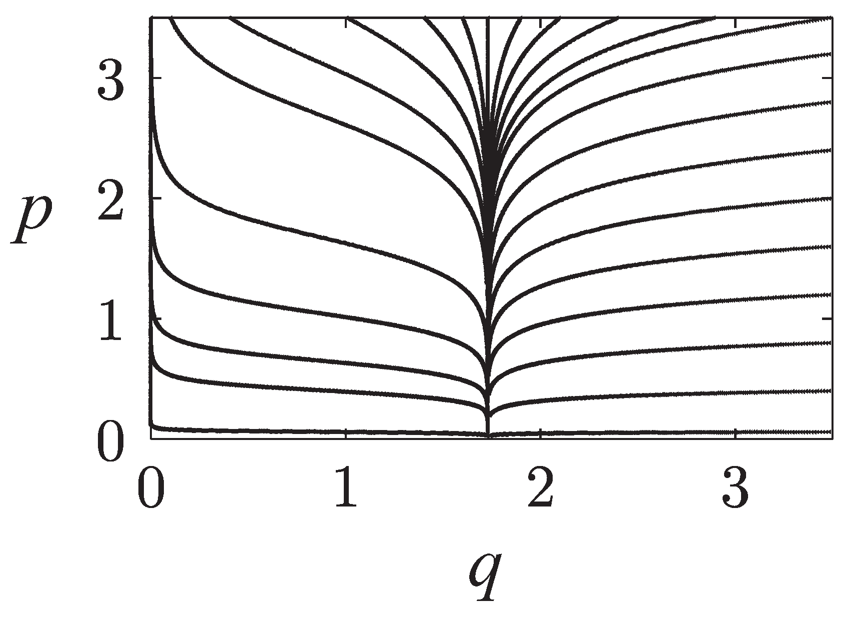
8]. The curves generated with the gradient of the Hamiltonian,
are shown in
Figure 1. The simplest curves are the ones located at the extremal points of the potential function, at
, where the force vanishes. At those points, the lines are parallel to the momentum axis, which is the coordinate eigencurve at the extremal sites.
Figure 1.
Normal curves to the energy surfaces for the nonlinear oscillator, with , and . We only show the positive q axis. Any of these curves can be used as an initial time curve, but the curves that correspond to the extremal points of the potential function () are the simplest ones: straight lines parallel to the coordinate axes.
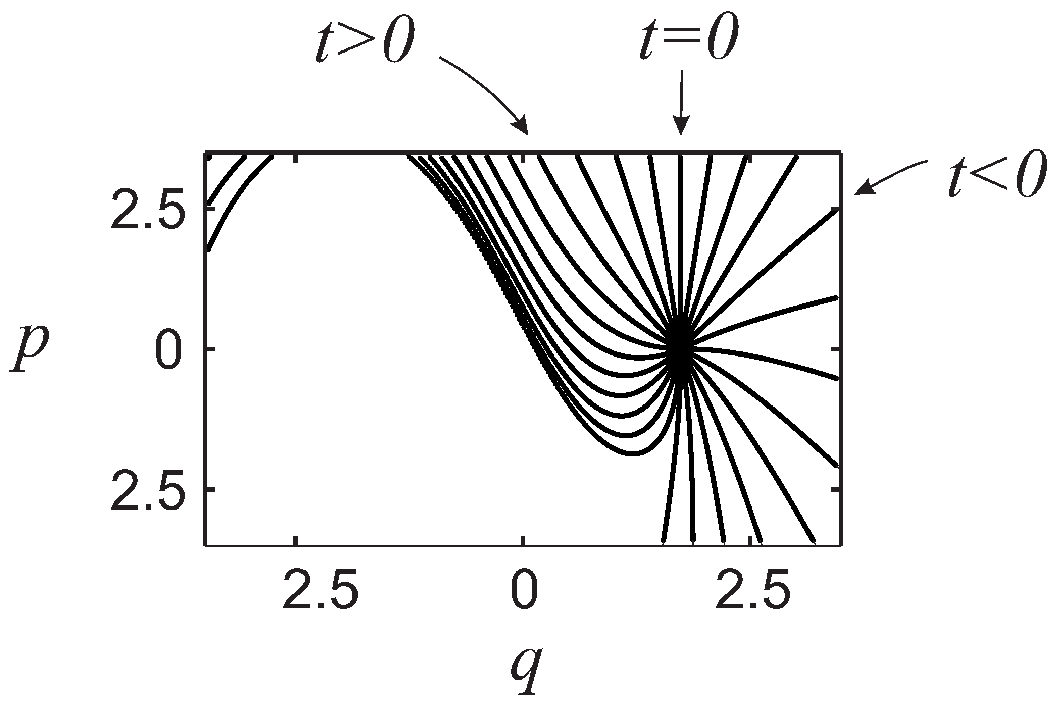
Therefore, we can take any of the curves passing through the extremal points as an initial time eigencurve and generate a time coordinate system with these curves. These curves will cross all the values of energy, a necessary condition for classical and quantum time eigenstates. By taking the line
as the initial time eigenstate, we generate the time coordinate system in phase space shown in
Figure 2. The idea of using a coordinate eigencurve at an extremal point of the potential function as the origin of time can also be used for quantum systems.
Figure 2.
A time coordinate system for the nonlinear oscillator, generated with the initial curve , with , and . These curves will cover the phase space several times because the system is periodic.
Figure 2.
A time coordinate system for the nonlinear oscillator, generated with the initial curve , with , and . These curves will cover the phase space several times because the system is periodic.
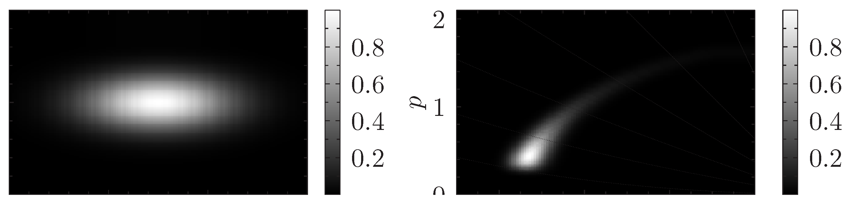
Because time and energy are simply another set of coordinates in phase space, a probability density will have widths along these directions. For instance, a Gaussian probability density in energy-time space, centred at
and given by
where
σ and
α are the density’s widths in time and energy, respectively, will correspond to a phase-space probability density that also has non-vanishing widths. This result is shown in
Figure 3.
Figure 3.
Density plots of the time-energy and phase-space representations of a time-energy Gaussian probability density for the nonlinear oscillator, with , and . The widths are non-zero in both representations.
Figure 3.
Density plots of the time-energy and phase-space representations of a time-energy Gaussian probability density for the nonlinear oscillator, with , and . The widths are non-zero in both representations.
Time evolution in energy-time space is simply a shift along the time axis without a change of the shape of the probability density. However, this action corresponds to symplectomorphisms that will change the shape of the probability density in phase space.
4. Quantum Systems
In quantum systems, we can also use coordinate eigenfunctions as the zero-time presence eigenstate. Let us rewrite the coordinate representation of a wave function as follows:
Thus, the wave function can be viewed as the projection of the ket
on the ket
. In the coordinate representation of the wave packet,
t is a parameter and the wave function has
q as the independent variable. However, we can fix the coordinate: let us say that
and that
t is the independent variable. We then define the time eigenstate as
Based on the results of the previous section, we propose to use the free-particle eigenstates at the location of the extremal points of the potential function as the zero-time eigenstates. At the extremal points, the Hamiltonian looks like the free-particle Hamiltonian.
If the zero-time value is assigned to the coordinate eigenstate
, where
X is one of the extremal points of the potential function, the kets generated with the propagator are the time eigenkets for other values of time. Assuming that the relationship
holds, we can show that the time eigenkets generated with the propagator are eigenfunctions of the time operator:
where we have made use of the property that
.
Denoting the time-reversal operator (complex conjugation and replacement
) by Θ, the time eigenstate is invariant under the following operation:
The time eigenvectors can be used to write the identity operator as
where we have set
,
i.e., a phase factor. This choice for
as a phase factor is fixing the state that should be used. Below, we will identify what these phase factors are (see Equation (
67)). We are using this particular state for the generation of a time coordinate for any potential function, just as for the classical case. Phase factors were also used by Bokes in the stroboscopic wave packet basis [
9,
10,
11,
12], and by Hegerfeldt and coworkers [
13].
A time operator is defined as
Because the time eigenstates are time reversal invariant, the time operator complies with the desired property:
The energy representation of the time operator can be readily found:
Thus, we have expressed the time operator in the time representation and in the energy representation.
The time operator found by Galapon is similar to our operator in the energy representation but without the oscillating factors [
14,
15,
16]. That operator complies with the commutator with the energy relationship but in a limited domain, and it is not clear what the eigenvectors of this operator are. Our operator emerges in a natural way and also complies with the requirements for a time operator. It is easy to see that the time operator is self-adjoint, and a finite Fourier transform of the time eigenvector is
the corresponding energy eigenvector. The discrete inverse transform of the energy eigenvectors, with the appropriate phases, is
Time eigenstates at the same time but generated with different zero time kets are orthogonal,
However, there are parts of the time eigenstate with zero momentum. These components with zero momentum will overlap for all time; as a result, the time eigenstates generated with the same initial eigenstates will not be orthogonal:
To determine the commutator between
and
, let us do the following
Thus,
The last term will vanish for large
T when applied to a wave function, assuming that the wave function is localised in a finite region of
t. This localisation is expected for
integrable functions. The boundary term will also vanish for
t-periodic wave functions. A state for which the boundary term might not vanish is an eigenstate of the Hamiltonian when the potential function is not periodic. However, eigenstates of some operators can become complicated as is the case of the momentum eigenstates, which are not normalisable. In those cases, we might consider the use of a limited set of eigenvalues to eliminate the boundary terms. In numerical studies we have to work in finite regions of phase space and then the boundary terms can be safely neglected.
Now, the free-particle energy eigenstate, in coordinate representation, is
These states are precisely what we need: a state such that
, where
and
. Thus, we can use a coordinate eigenstate placed at any point but it would be better, however, to place the eigenstate at the locations of the extremal points of the potential function, in accordance with the discussion of the previous section. With this choice, we ensure that the time eigenstate will be formed with all of the energy eigenstates. A coordinate eigenstate with origin at other points will most likely not contain all of the energy values.
Finally, we note that we can derive similar results for the cases of degeneracy of the energy eigenfunctions and for continuous energy spectra [
13].
5. Conclusions
We have introduced a change of variables to simplify the description of the time evolution of a classical system; this method differs from a canonical transformation. Canonical transformations are intended to preserve the form of Hamilton’s equations of motion, whereas the variables are changed; the time variable remains a parameter. However, our transformation changes to a set of variables in which the motion in time does not require an extra parameter. This transformation reduces the number of variables required to follow time evolution, one of which is the time variable.
We note that in the phase-space coordinate system, the constant momentum curves encompass all the coordinate values, and vice versa. Similarly, the constant time surfaces should cross all values of energy, unless we are interested in a subset of the energy values. A way to ensure this property is to follow the normal direction to the constant energy shells. These curves can become very complicated; therefore, we have found the simplest curves, the lines parallel to the momentum axis placed at the extremal points of the potential function. At the location in which there is no force, the particle behaves as a free particle; the free-particle presence eigenfunctions can also be used in the non-free case. The free-particle coordinate eigenstates have been used previously, but in this paper we have found the best location for these surfaces.
Thus, we propose the use of conjugate “proper coordinates": the time-energy hypersurfaces. These coordinates led to a simpler analysis of the motion of points and functions in phase space.
Our treatment also sheds light on the way in which we can address time in quantum systems: to generate the time eigenfunctions by starting with the free-particle eigenfunction placed at the zero-force location. We can also use the free-particle eigenfunctions if these functions are placed at other sites, however, these eigenfunctions might not contain all of the energy values.
These results can be extended to more dimensions than one. In the case of more dimensions, we fix one of the coordinates obtaining a hypersurface in phase-space, and we will end up with one less variables to deal with.
We also mention that we can use a finite range of energy values for the time eigenstates. In that case, the curves will be contained in a finite region of phase space, which is suitable for numerical calculations.
These results are also applicable to the so-called Maxwell Hamiltonians, which are Hamiltonians of the form
where the conjugate moment
p is defined by
Our approach to the correspondence between classical and quantum mechanics is different from earlier approaches [
17,
18] because we are simply using objects that are already part of these theories but that have not yet been explored.
The phase factors attached to the energy eigenfunctions allow the placement of the initial time eigenstate at any chosen location, and we have shown the best locations in which to place the initial time eigenstate.

