Article

Entropy of Shortest Distance (ESD) as Pore Detector and Pore-Shape Classifier

1
Earth Sciences Department and Reservoir Characterization Research Group, King Fahd University of Petroleum and Minerals, Dhahran 31261, Saudi Arabia
2
Russian-French Metallogenic Laboratory, 11-11 Mokhovaya Street, Moscow, 125009 Russia
3
Centro de Geociencias, Universidad Nacional Autónoma de, México (UNAM), Km. 15.5, Carretera Querétaro-San Luis Potosí, C.P. Juriquilla 76230, Querétaro, Mexico
4
Vernadsky State Geological Museum of Russian Academy of Sciences, 11-11 Mokhovaya Str., Moscow, 125009 Russia
*
Author to whom correspondence should be addressed.
Entropy 2013, 15(6), 2384-2397; https://doi.org/10.3390/e15062384
Submission received: 25 March 2013 / Revised: 7 May 2013 / Accepted: 15 May 2013 / Published: 10 June 2013
(This article belongs to the Special Issue Applications of Information Theory in the Geosciences)

Abstract

:
The entropy of shortest distance (ESD) between geographic elements (“elliptical intrusions”, “lineaments”, “points”) on a map, or between "vugs", "fractures" and "pores" in the macro- or microscopic images of triple porosity naturally fractured vuggy carbonates provides a powerful new tool for the digital processing, analysis, classification and space/time distribution prognostic of mineral resources as well as the void space in carbonates, and in other rocks. The procedure is applicable at all scales, from outcrop photos, FMI, UBI, USI (geophysical imaging techniques) to micrographs, as we shall illustrate through some examples. Out of the possible applications of the ESD concept, we discuss in details the sliding window entropy filtering for nonlinear pore boundary enhancement, and propose this procedure as unbiased thresholding technique.

1. Introduction

In the early years of Information Theory, Good ([1,2], see also [3,4]) introduced the influential “how to keep the forecaster honest” paradigm, that is how to design a payoff system which would force the forecaster to give an unbiased prediction. Much later (in 1972 [5]) it was proved mathematically that the only way to do this is intimately connected with the concept of Shannon entropy.

1.1. Motivation

In the parlance of Petroleum Exploration, permeability—one of the most important petrophysical property of reservoir rocks, and the principal target of our recent research—is never “estimated” or “computed” from well logs, well pressure transients, or small cuttings of rock: it is always “predicted”. There is, of course, a hidden caveat in the term: any prediction can go wrong. Soothsaying is a dangerous business. In Dante's Inferno the souls of soothsayers who misled their clients have their heads twisted to the rear, so they walk backward. But it is so easy to understand why the diviners had cheated. Who would dare to upset a Caesar who ordered “Go bid the priests to do present sacrifice; And bring me their opinions of success” (Shakespeare: Julius Caesar II, 2,5—italics ours; the last three sentences are paraphrased from the study [6]).

2. Methodology

2.1. Mathematical Model

Let the probability of the ith possible event be p i , i = 1 , , N and suppose the forecaster gets a payoff f ( p i ) , i = 1 , , N if he predicts this event, that is his expected payoff is p i f ( p i ) . If we want to keep the forecaster honest, we must select a function f ( p i ) such that for any other probability distribution q i , i = 1 , , N one has:
p i f ( p i ) p i f ( q i )
that is, the expected payoff is maximal if the forecaster predicts the events according to their correct probability. In a brilliant paper, Pál Fischer [5] proved that the only function satisfying Inequality (1) is f ( p ) = c o n s t ln ( p ) that is—apart from a constant factor—the expected payoff is the Shannon entropy H = p i f ( p i ) . Putting aside the “forecaster” analogy, we can say that the only reasonable and unbiased quantitative "value" what we can associate with the information about a probability distribution p i , i = 1 , , N is its entropy, H = p i f ( p i ) .
This consideration had been one of the motivations for our group to introduce, some 10 years ago, the TRISA relative-entropy triangle to analyze and conveniently plot the joint development and mutual dependency of three variables, measured in incommensurable units [7,8]. In the present paper we use Shannon entropy in a very different context, as a measure of the structural (configurational) disorder of random geometrical patterns [
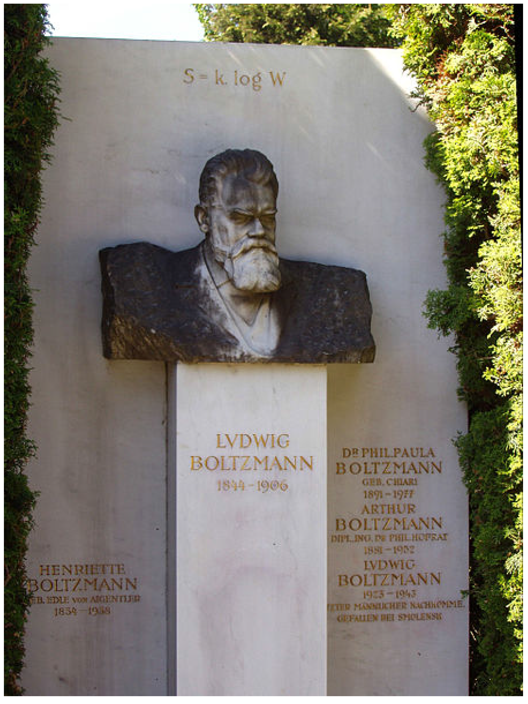
9]. In the statistical physics of point patterns configurational entropy is defined as S = k B ln W where W is the number of different configurations, assuming that all configurations are equally probable (Boltzmann's equation, k B is the Boltzmann constant, Figure 1). If the configurations have different probabilities p i , i = 1 , , W then combinatorial reasoning and application of the Stirling’s approximation yield S = k B i = 1 W p i ln p i ([10,11]).
Figure 1. Ludwig Boltzmann’s grave in the Central Vienna Cemetery, with his famous equation, S=k log W.
Entropy 15 02384 g001
In the geometrical probability theory of irregularly placed points the distances to nearest neighbor, and their probability distribution, have become a standard tool to characterize spatial relationships in populations [12]. It was first proved by Hertz ([13], simplified in [12]), that if a large number of points are Poisson-distributed on the plane with density ρ, and for every point P i , i = 1 , , N its distance to the nearest neighbor is r i then the average value of r i , that is r A v = 1 N 1 N r i , tends to an expected value r E for N :
lim N r A v = lim N 1 N r i N = 1 2 ρ = r E
Thus, the randomness of a point arrangement can be characterized by the ratio [12]:
R = { 1 N r i N } : 1 2 ρ = r A v r E
For a completely random point distribution R = 1 , if all points are at the same position then R = 0 , for periodical arrangements one can have R > 1 (such as R = 2 for a square lattice, R = 2.1491 for the hexagonal lattice, [12]).
Another convenient measure of irregularity is the Shannon-entropy of the distribution of nearest neighbor distances { r i } . For a regular square lattice, all distances { r i } are equal, and the Shannon entropy of the distance-to-nearest-neighbor distribution is 0. The more irregular is the lattice, the larger will be the variation among the values { r i } , and consequently, the larger will be the Shannon entropy of their distribution. If, for a randomly selected point P i , and any x 0 we have, independently of the index i, that Pr { x min j [ d i s t ( P i , P j ) | j i ] x + d x } = r ( x ) d x where 0 r ( x ) 1 ; 0 r ( x ) d x = 1 and Pr means probability of a random event, dist is the Euclidean distance, then:
H = 0 r ( x ) ln r ( x ) d x
is a meaningful (and, as we discussed above in connection with the forecaster problem, the only objective) measure of the irregularity of a point distribution.
The intimate connection between distance-to-nearest-neighbors and entropy is expressed by a Theorem of Kozachenko and Leonenko ([14,15,16]) which states that, under some mild conditions, for N points distributed in the d-dimensional Euclidean space:
H N , d = d N i = 1 N ln r i + ln [ π d / 2 Γ ( 1 + d 2 ) ] + γ + ln ( N 1 )
where H N , d is the entropy of the d-dimensional point distribution, the factor in square brackets is the volume of the d-dimensional unit sphere, γ = 0.5772 …. is Euler's constant, Γ the gamma function. For the 2-dimensional case:
H N , 2 = 2 N i = 1 N ln r i + ln π + γ + ln ( N 1 )
By the inequality between the geometric and arithmetic means of positive numbers ([17])
1 N i = 1 N ln r i = ln r 1 r N N ln r 1 + + r N N = ln r A v , which gives an upper bound for the entropy of an arrangement of N points:
H N , 2 2 ln r A v + ln π + γ + ln ( N 1 )

2.2. Entropy of the Shortest Distance

In Economic Geology, Geochemistry, and Mineral Exploration there are legions of empirical rules, which claim cause-effect relations between observable planar objects (such as faults, lineaments on aerial photographs; halos with increased radon activity, etc.) and the presence of proved mineral occurrences [18,19,20,
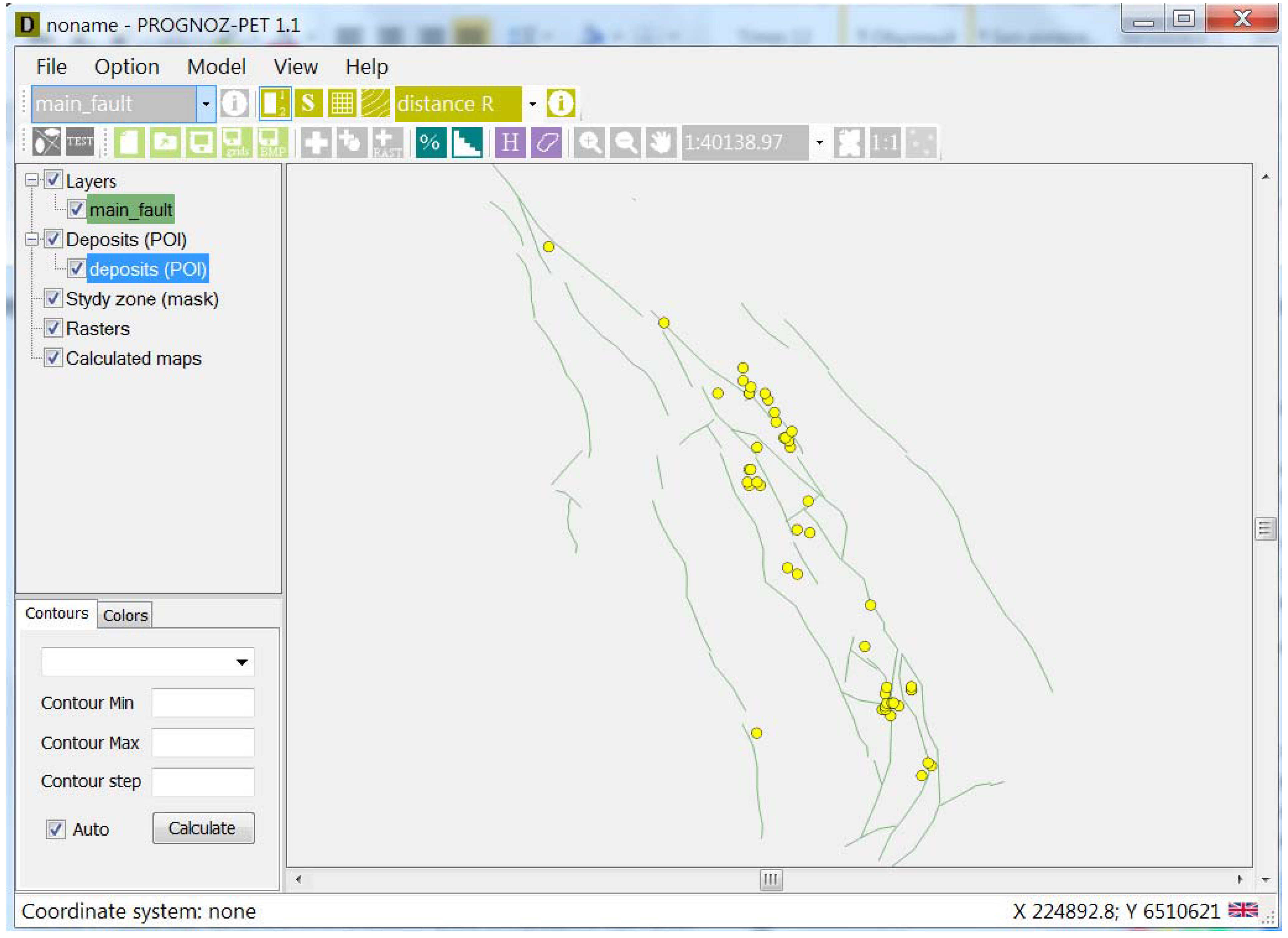
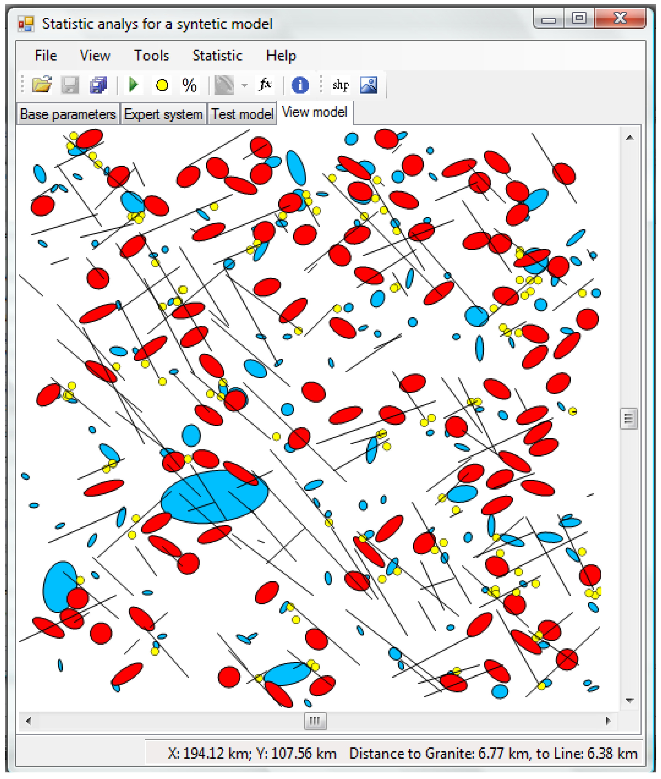
21]. A hypothetical case is shown in Figure 2 where the lineaments (green lines) are apparently related to mineral occurrences (yellow dots). In the spirit of the "entropy of shortest distance" we expect that if the distances of the dots from the nearest lines are very randomly distributed, with large entropy, then there is no valid relation between the two sets of objects. On the other hand, if all distances are small, within the measurement accuracy only a few different values will be observed, and the distribution will have a small entropy. Thus, a low entropy of shortest dot-to-line distances would prove the causal relation between the two sets. The idea can be easily extended to three kinds of randomly distributed objects (“ellipses”, “lineaments”, “points”), see Figure 3.
Figure 2. A model representing the case of strong correlation between the placement of the mineral occurrences (yellow dots), and lineaments.
Entropy 15 02384 g002
Of course other, metric approaches are also possible [12,18], based on the actual values of the shortest dot-to-line distances, their distribution, mean, their normality, etc. Still, as discussed previously, by Fischer’s [5] Theorem only the entropy can be considered as an objective measure.
The ESD (entropy of shortest distance to neighboring element) idea was studied in depth in the PhD thesis of B. Sterligov [22] then it has been further developed, in collaboration with Professors S. Cherkasov and K. Oleschko to the user friendly PROGNOZ software [
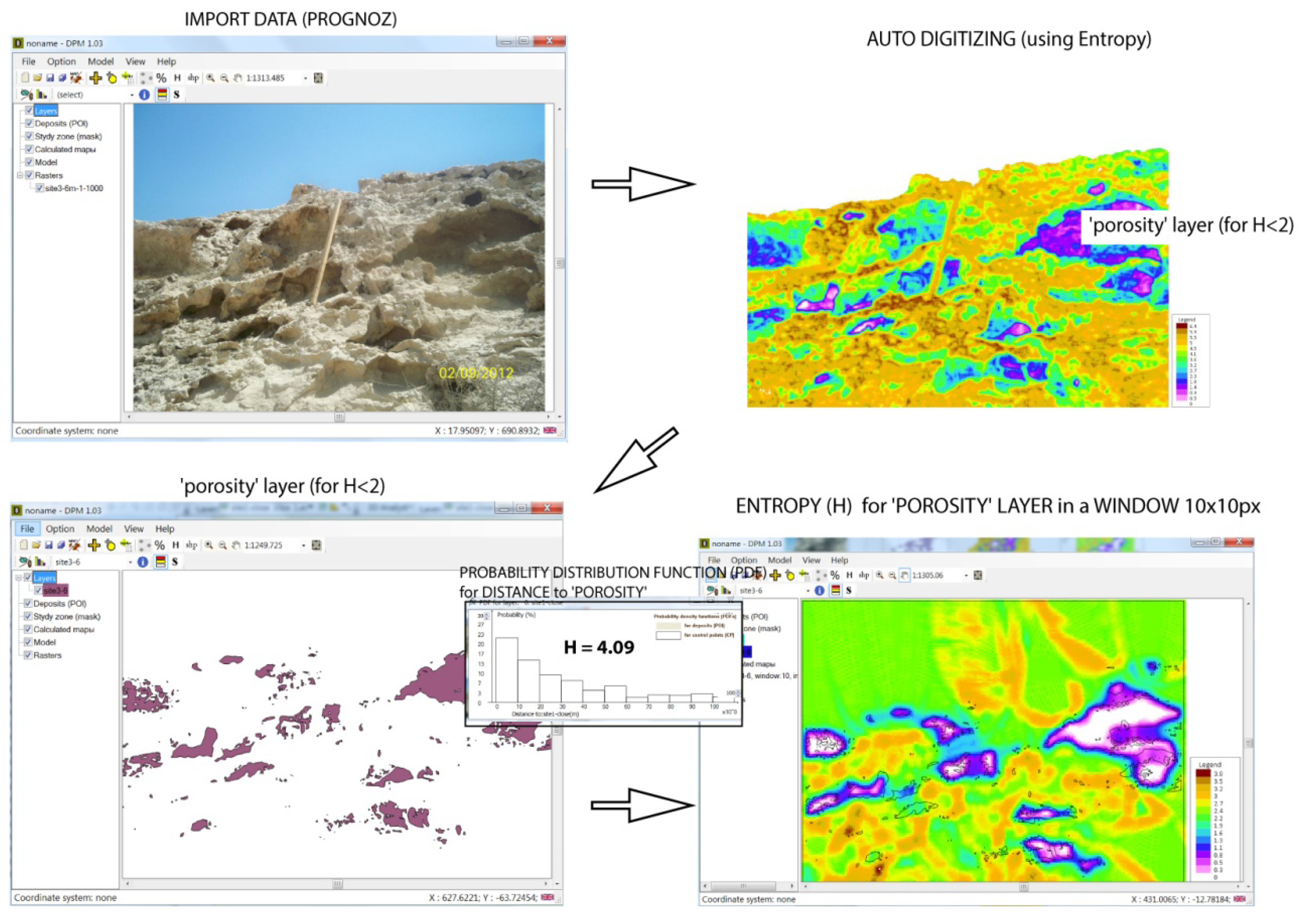
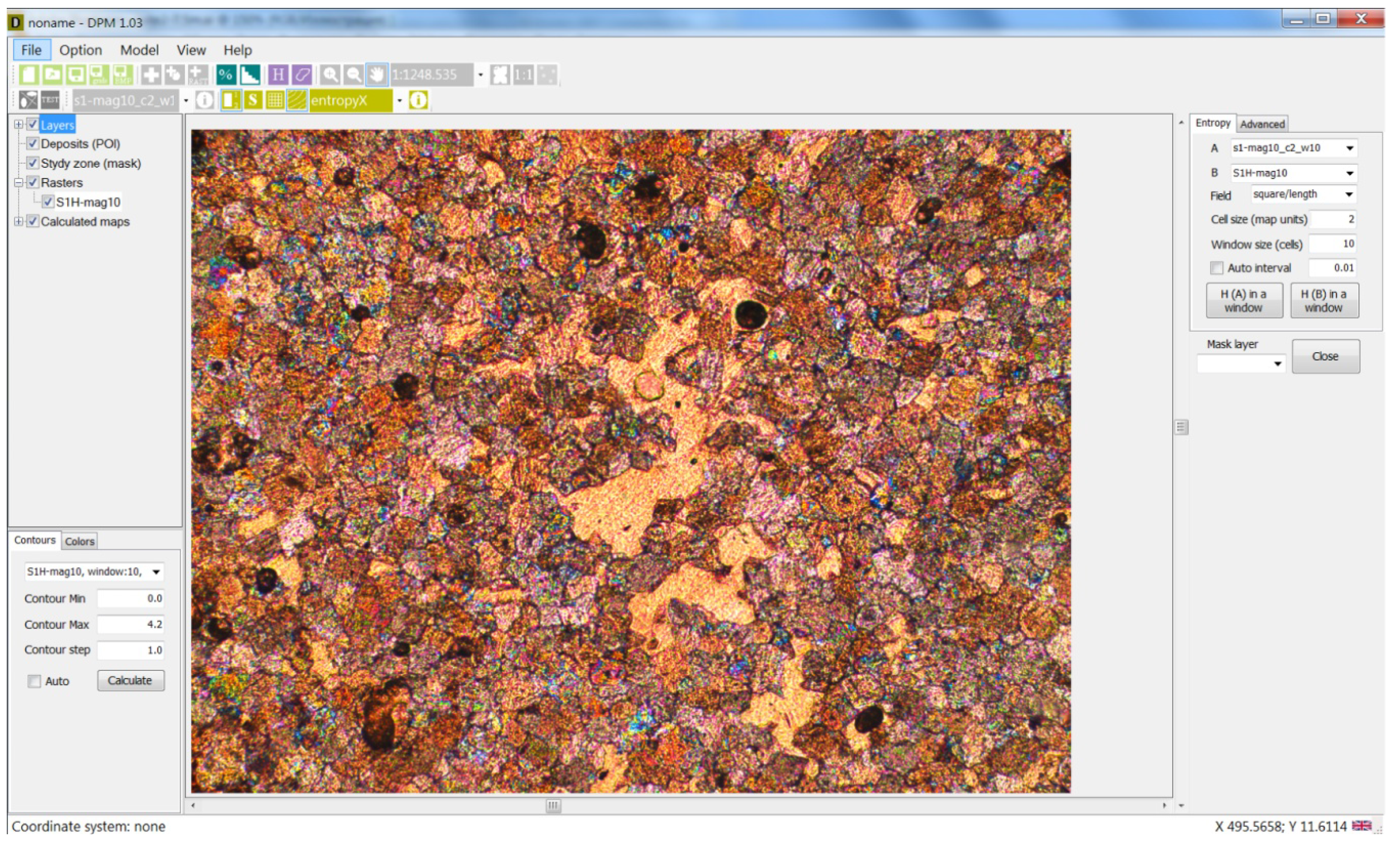
23]. Quite recently, we realized that making an analogy between the three geographic elements “ellipses”, “lineaments”, "points" and the macro- and microscopically observable “vugs”, “fractures” and “pores” of triple porosity naturally fractured vuggy carbonates, we get a powerful new tool for the digital processing, analysis, and classification of the void space in carbonates, and other reservoir rocks. The procedure is applicable at all scales, from micrographs to outcrop photos, as we shall illustrate by examples.
Out of the many possible ways to apply the ESD concept, we only discuss the sliding window entropy filtering for pore boundary enhancement, in the next Section. A similar technique, based on the ESD of Poisson distributed random points from nearest pores, will be briefly mentioned in the concluding part.
Figure 3. Spatial relation between three shapes ("granite outcrops" blue, "mineral occurrences" (red), and "lineaments", black). Scaled down by a factor 10 5 , the model might represent an outcrop of a vuggy, fractured limestone (see Figure 7), reducing it by 10 8 it will resemble an optical micrograph of a triple porosity carbonate (Figure 8, Figure 9). Our entropy technique remains applicable through this enormous range of scales.
Entropy 15 02384 g003

2.3. Sliding Window Entropy Filtering for Bore Boundary Enhancement

Using the standard notation of geometry [24,25,26] if A and B are sets in the n-dimensional Euclidean space R n of finite measure μ ( A ) < , μ ( B ) < , then the Minkowski sum of A and B is defined as:
A B = x A ; y B ( x + y )
In the special case when B is the n-dimensional hypersphere, we call S ( r ; A ) = A B the extended hypersphere of radius r around A. In the 2-dimensional (planar) case, assuming that the set A is convex, and denoting the length of its circumference by c(A), by a Theorem of Tomiczková [26] the area of the extended circle S ( r ; A ) is given by:
μ { S ( r ; A ) } = μ ( A ) + μ ( B ) + r c ( A ) = μ ( A ) + r 2 π + r c ( A )
where in the 2-dimensional case μ 
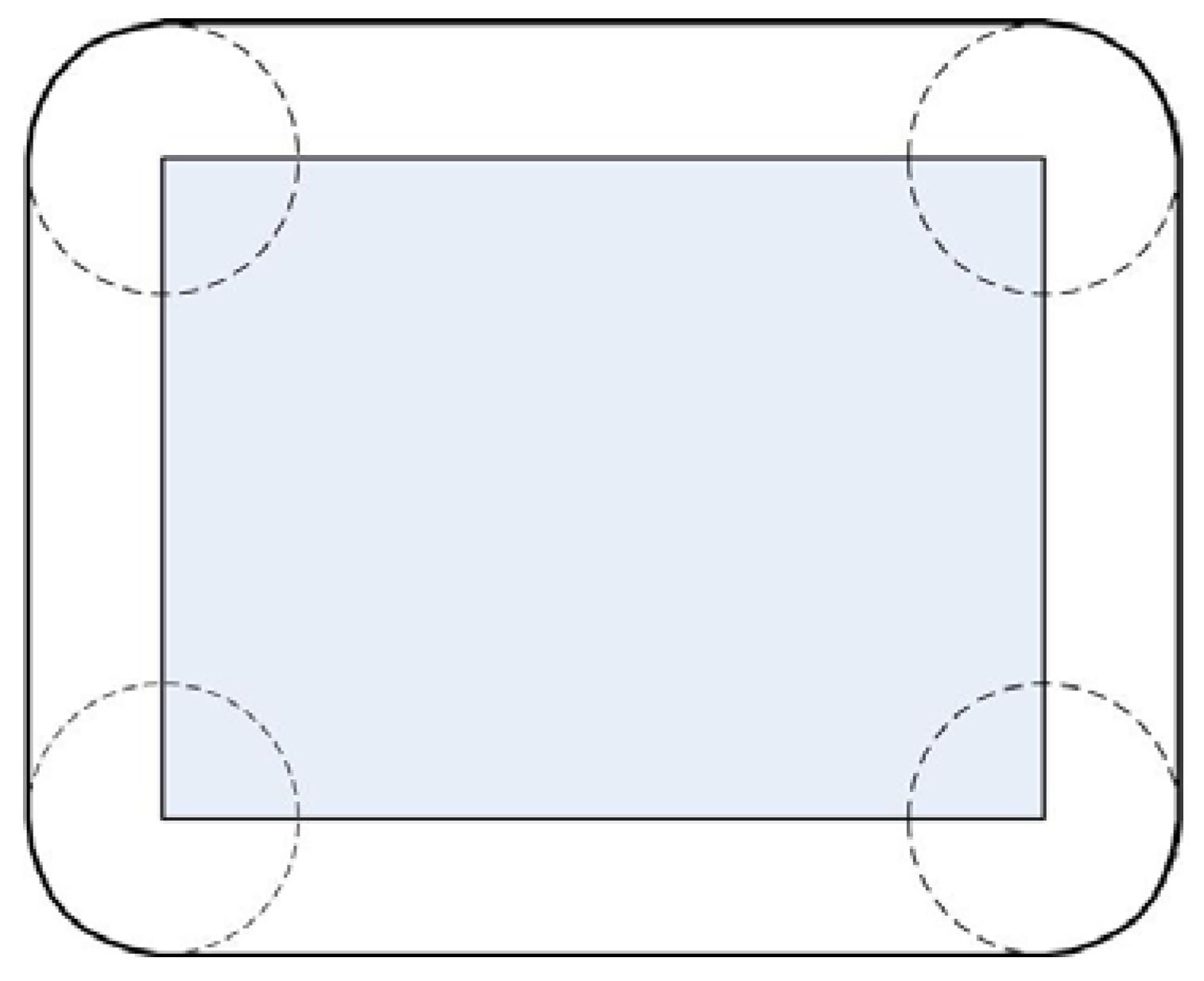
is area. An example of “extended circle” around a rectangle is shown in Figure 4. If the radius of the circle B is r, the sides of the rectangle A are a and b, it is easy to check Equation (7) because μ ( A ) = a b , μ ( B ) = r 2 π , c ( A ) = 2 ( a + b ) and, directly from the figure, μ ( A B ) = a b + 2 r a + 2 r b + r 2 π .
Figure 4. Minkowski sum of a rectangle of sides a, b with a circle of radius r ( r < a , r < b ).
Entropy 15 02384 g004
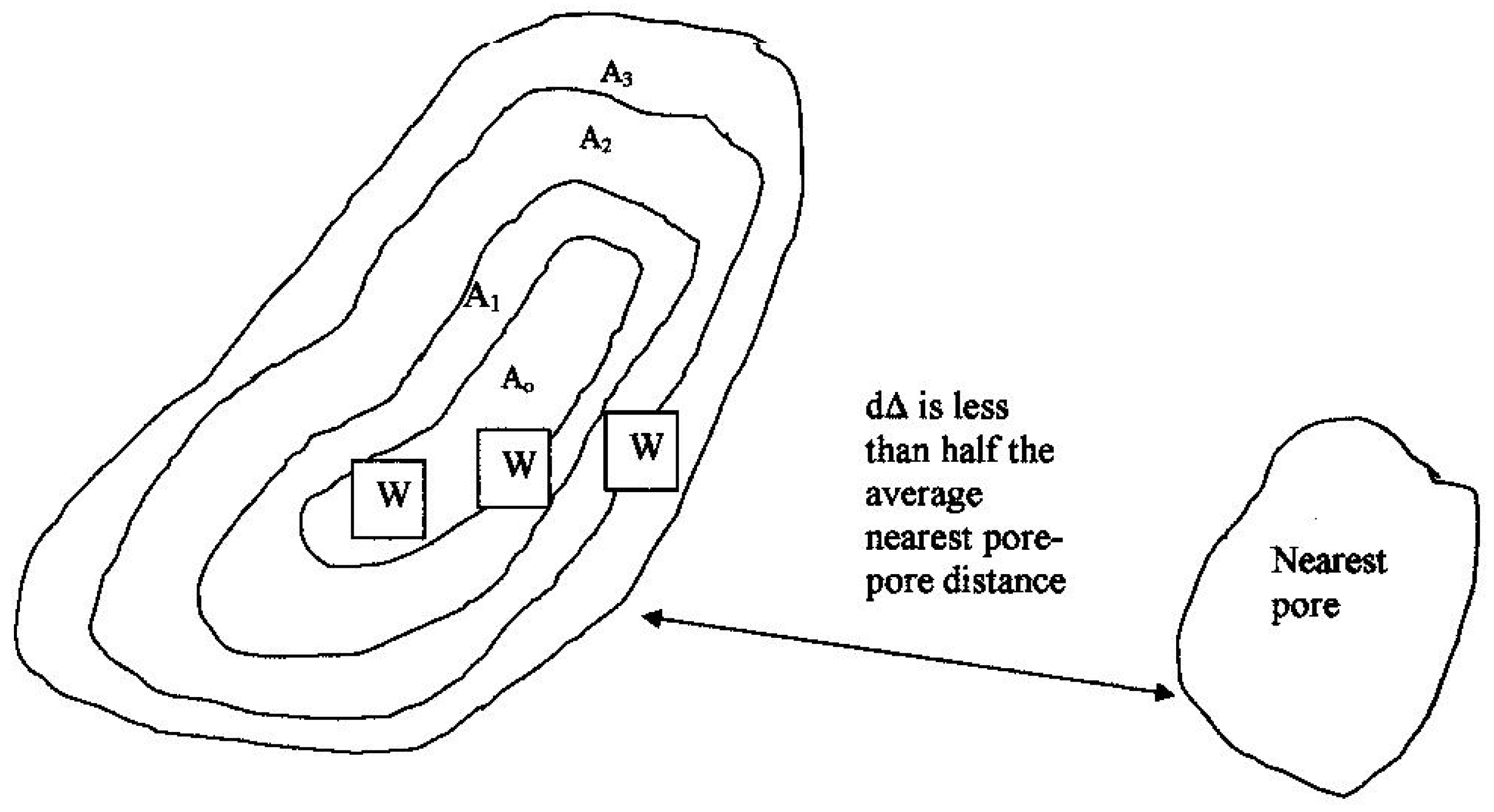
Consider now a "pore" A in the digital image, suppose the distance of A from the nearest pore is D. Let Δ denote pixel size, select a reasonably large ( w Δ × w Δ ) -size (say 10 × 10 pixels) window W, where w Δ is less than half the distance of A from the closest pore, i.e. w Δ D 2 = K Δ , but at the same time it is much less than the size of the pore A. The "pore" in the image is distinguished with a separate color, or a distinct range of values of gray scale. The boundary of the pore is generally diffuse, not clearly defined because of non zero thickness of the thin sections (which commonly measured less than 30 μm). Let us consider the sequence of extended circles with increasing radii around A (see Figure 5):
The sequence of these sets satisfies (where in the 2-D case the measure μ is area):
A = A 0 A 1 A K   and   μ ( A ) < μ ( A 1 ) < < μ ( A K )
Taking set-theoretical differences between successive extended spheres around A of respective radii k Δ and ( k 1 ) Δ we get a sequence of rings ρ 1 , , ρ K ( k = 1 ; 2 , , K ) around the pore A defined as: ρ k = A k \ A k 1 ( k = 1 , , K ) . By the construction, each ring is one pixel wide. If the moving window W is closer to the pore A than D/2 then:
W = ( W A ) ( W ρ 1 ) ( W ρ K )
and, consequently, (because the rings are distinct):
μ ( W ) = μ ( W A ) + i = 1 K μ ( W ρ i )
Figure 5. Illustration of the sliding window entropy technique for a better definition of the boundary of the pore A 0 . The sliding window W, which moves out of A 0 , has a size less than half the distance to the nearest pore. The sequence A 0 A 1 A N is strictly increasing, the difference sets ρ k = A k \ A k 1 ( k = 1 , , N ) form one pixel wide “rings” or “halos” around A 0 .
Entropy 15 02384 g005
A 0 = A = S ( 0 ; A ) A 1 = S ( Δ ; A ) A 2 = S ( 2 Δ ; A ) A K = S ( K Δ ; A ) = S ( D / 2 ; A )
Suppose the square-shaped window W moves, without rotation, staying parallel to its original position, along a linear path as shown in Figure 5. In the figure, W starts to move from a position where it is fully inside A, W A , then it passes through intermediate positions when only a part of W is inside the pore: W A ∅, up to a final position when W is fully outside the pore and it is covered by M successive rings: W A = ∅ and A i = k k + M 1 ρ i ; k 1 .
In any position of the moving window, the altogether w 2 pixels in W define the set of w 2 distances { δ 11 , δ 1 w , , δ w 1 , , δ w w } where δ i j is the shortest distance (with the precision of pixel-size Δ) between the pixel p i j W , i , j = 1 , 2 , , w and the pore A. Considering these distances as random variables, any δ i j can take a value from among the possible distances { 0 , Δ , , K Δ } and we can compute their empirical probability distribution { p 0 , p 1 , , p k , , p K } as:
p k = # { δ i j | δ i j = k Δ } / w 2
where # { S } denotes the number of elements of the set S. The Shannon entropy of this distribution is H = k = 1 K p k ln p k , with the usual convention that for p = 0 the product p ln p is defined as lim p 0 p ln p = 0 . Consider the three possible positions of the window W relative to the pore A.
If W is fully inside A then all distances δ i j are 0, so that { p 0 = 1 , p 1 = = p K = 0 } and H = 0 .
If W is fully outside A but still inside the extended sphere of radius K Δ around A, then in a typical case it will have non-empty intersections with w consecutive rings:
W ρ i ≠∅  for  i = k , k + 1 , , k + w 1
for some value of k in such a way that each intersection with a ring ρ i contains about w pixels, and in the set W ρ i all distances are equal to the same value δ i = i Δ . In this case, the typical probability distribution will be:
{ p i = w / w 2 = 1 / w f o r k i k + w 1 a n d p i = 0 o t h e r w i s e }
The corresponding Shannon entropy is:
H i = k k + w 1 1 w ln 1 w = ln w
Consider now the most interesting case, when part of the window W lies inside pore A, the rest of it is outside in such a way that it has non-empty intersections with the first l rings only: W A ∅, W ρ i ∅ for i = 1 , 2 , , l where l < w . In a typical case each intersection with a given ring ρ i contains about w pixels, and in the set W ρ i all distances are equal to the same value δ i . In this case the probability distribution is:
{ p 0 = w 2 w l w 2 ; p 1 = = p l = 1 w a n d p i = 0 o t h e r w i s e }
which yields the entropy:
H ( 1 l w ) ln ( 1 l w ) + l w ln w
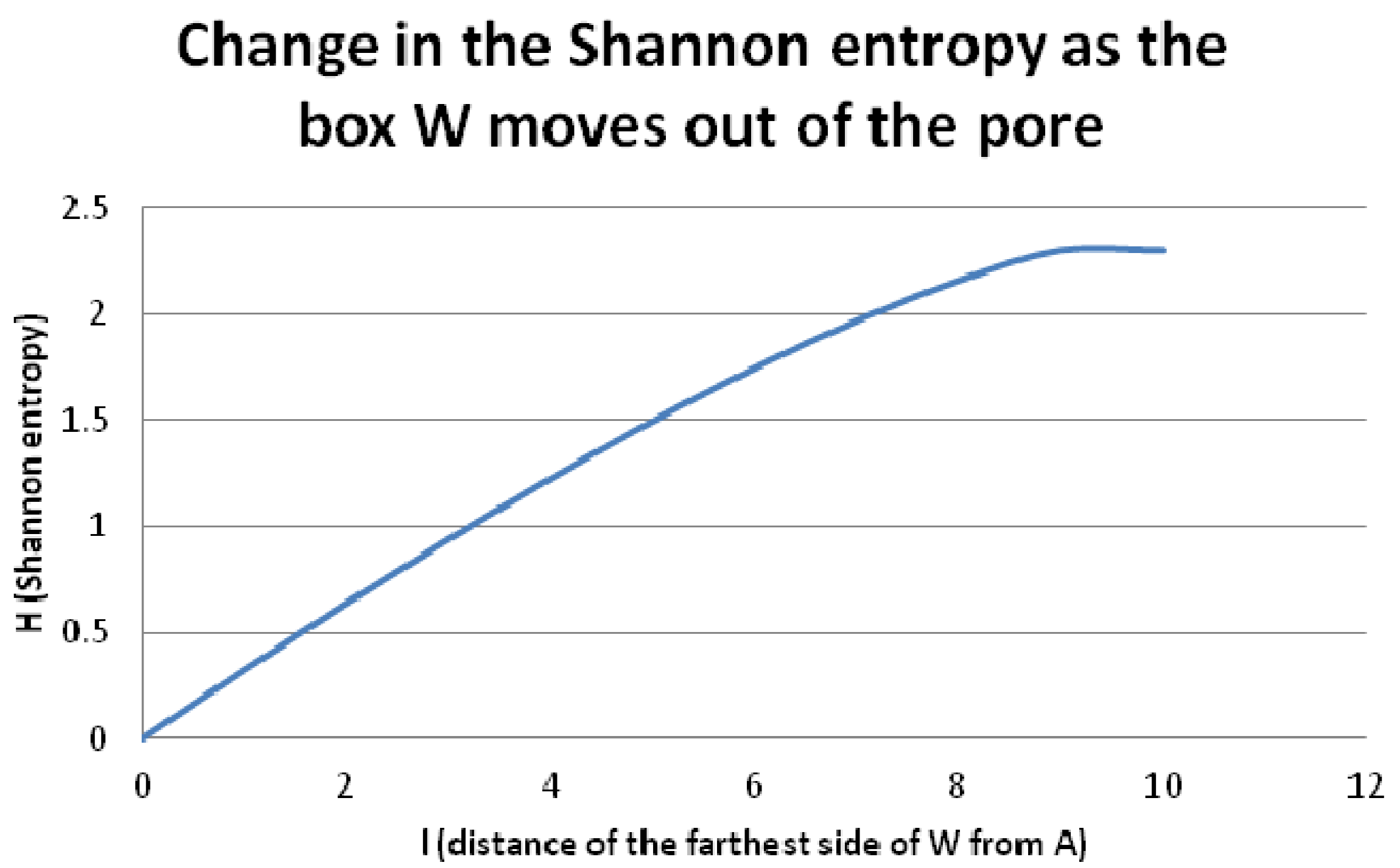
Figure 6 shows how the Shannon entropy (Equation (17)) increases as the box W gradually moves out from the pore, for the case when W consists of 10 × 10 pixels. We emphasize that in order to compute the entropy, we do not have to actually construct the rings around the pore, but we do need an algorithm to find the distance of any pixel from the nearest pore.
As seen from the graph (Figure 6), we can use the following algorithm to define the boundary A of the pore A: Select the size of W less than the half distance between nearest pores. In any position of the moving window W compute the distances { δ 11 , δ 1 w , , δ w 1 , , δ w w } of its w 2 pixels from the nearest pore with the precision of pixel-size Δ. Define the probability distribution of the different distances, { p 0 , p 1 , , p k , , p K } , where p k = # { δ i j | δ i j = k Δ } / w 2 , (see Eq. 12), and calculate the corresponding Shannon entropy H = k = 1 K p k ln p k . When W is fully inside a pore, then H = 0 , when W is moving out of the pore, step by step, the entropy of distances from the pixels of W to the pore will increase to ln w (according to Equation (17)). The maximal possible entropy of the distribution of distances { δ 11 , δ 1 w , , δ w 1 , , δ w w } would occur when all δ i j are different and equally probable, and this would be twice as large as H in Equation (15):
H max = i = 1 w j = 1 w 1 w 2 ln 1 w 2 = 2 ln w
If we select W as consisting of 10 × 10 pixels, then in Eq. (15) we have ln d = ln 10 = 2.303 , and it is a reasonable criterion to define the interior of the pore with the inequality H = k = 1 K p k ln p k 2 . More generally, using a w × w - sized window, the boundary of the pore is defined by H = k = 1 K p k ln p k ln w .
Figure 6. Change of the Shannon entropy (Equation (17)) as W gradually moves out from the pore.
Entropy 15 02384 g006

3. Examples, Discussion, and Outlook

3.1. PROGNOZ Application to Pore Boundary Detection

The entropy technique has been incorporated in our PROGNOZ software package [23]. It has proven successful in different applications. It can be used for images at any scale as seen in Figure 7 and Figure 9, where Figure 7 is the photo of a carbonate outcrop from Saudi Arabia (lower Eocene Rus Formation, described in [27]), Figure 9 is the ESD map of the optical micrograph (shown in Fig. 8) of a sample taken from the same outcrop. As seen in the 3rd image of Figure 7, the entropy cutoff H 2 reliably defines the “pores” (more exactly, vugs and caves in this case, as the picture represents the outcrop scale). The inset in Figure 7 shows the histogram of distances from randomly selected points to the nearest pore. To compute a histogram such as this, it is not necessary to move a sliding window W all over the image, we only need to randomly generate a large number of Poisson distributed points and compute the entropy of the probability distribution of their distances from the nearest pore. The mathematical treatment of the Poisson-distributed points approach is very challenging, and we have not attempted it in this paper. Mark Berman [25] derived the distribution of the distances of a fixed point from Poisson-distributed objects of random sizes and directions, as well as the distribution of distances between a fixed object and random Poisson-distributed points. We think that his results, combined with Tomiczková’s [26] Equation (7) for the area μ { S ( r ; A ) } will form the foundations upon which the theory of ESD of random Poisson-distributed points from the nearest pore will be developed.
Figure 7. Entropy of shortest distance (ESD) processing of a carbonate outcrop photo. The second image in the sequence shows the entropy map over the whole image, as discussed in the text, the cutoff H 2 defines the pores (3rd image). The inset shows the histogram of distances from randomly selected points to the nearest pore.
Entropy 15 02384 g007
Figure 8. 10 × magnification of a rock sample, taken from the outcrop in Figure 6. The position of the section is perpendicular to the face of the rock wall.
Entropy 15 02384 g008
Figure 9. Entropy of shortest distance (ESD) isolines of the micrograph on Figure 7. The ranges of entropy values are different for the various objects: Large vugs (H = 0.2–0.7), small vugs and pores (H = 1–1.7), solid matrix (H = 1.9–2.4).
Entropy 15 02384 g009

3.2. Concluding Remarks and Outlook

For triple-porosity carbonate rocks, apart from detecting void spaces on images, we also have to differentiate between pores, fractures and vugs. We expect that these three types of void space will be characterized by different entropy cutoffs. Some preliminary results are shown in Figure 9 representing the entropy map of the micrograph Figure 8, where we found for large vugs H = 0.2–0.7, for small vugs and pores H = 1–1.7, while in the solid matrix, far away from pores H = 1.9–2.4. For fractures, we expect a small entropy cut-off H 0 . Of course, these ranges depend on the size of the sliding window, what in our case was 10 Δ × 10 Δ . Both algorithms (the sliding window, and the Poisson points) are based on entropies of the probability distribution of the shortest distances of points from pores, rather than on entropies of these distances themselves considered as random variables. As compared to the entropy of the geometric distribution of N points on the plane (Equation 5b), which logarithmically scales with magnification λ:
H N , 2 ( λ ) = 2 N i = 1 N ln λ r i + ln π + γ + ln ( N 1 ) = 2 λ + 2 N i = 1 N ln λ r i + ln π + γ + ln ( N 1 ) = H N , 2 ( 1 ) + 2 ln λ
(the upper bound of entropy in Equation (5c) has a similar scaling) both our ESD measures are scale free, as for example the entropy map in Figure 9 only depends on the image in Figure 8 and not on its scale. Still, we would hesitate to call these algorithms scale invariant, because the cut-off entropy values characterizing pore- (or vug-, or fracture-) boundaries certainly depend on metric factors, which are the window size in the sliding window algorithm, and the density when we use Poisson-distributed points.

Acknowledgments

Financial support from the Project #168638 SENER-CONACYT-Hidrocarburos Yacimiento Petrolero como un Reactor Fractal (Project Leader Dr. Klaudia Oleshko) is gratefully acknowledged. The partial support was obtained from the PAPIIT program UNAM, México (the Grant IN 112812, Fractal Metrology). GK is thankful to his home Institution, KFUPM, and to the UNAM Campus, in Juriquilla, Qto., Mexico, for the peaceful and creative atmosphere for research at both places. The two anonymous Reviewers have done a wonderful job, what we gratefully appreciate.

Conflict of Interest

The author declares no conflict of interest.

References

  1. Good, I.J. Rational decisions. J. Roy. Stat. Soc. Ser. B 1952, 14, 107–114. [Google Scholar]
  2. Good, I.J. Uncertainty. and Business Decisions; Liverpool University Press: Liverpool, UK, 1954. [Google Scholar]
  3. Aczél, J.; Daróczy, Z. On Measures of Information and Their Characterization; Academic Press: New York, NY, USA, 1957. [Google Scholar]
  4. McCarthy, J. Measures of the value of information. Proc. Natl. Acad. Sci. USA 1956, 42, 654–655. [Google Scholar] [CrossRef] [PubMed]
  5. Fischer, P. On the inequality p i f ( p i ) p i f ( q i ) . Metrika 1972, 18, 199–208. [Google Scholar]
  6. Korvin, G. The value of information in the interactive, integrative and evolutionary world model: A case history. Humanomics 2000, 16, 15–24. [Google Scholar] [CrossRef]
  7. Oleschko, K.; Korvin, G.; Figueroa, B. Entropy based triangle for designing sustainable soil management. In Proceedings of 17th World Congress on Soil Science, Bangkok, Thailand, 14–20 August 2002.
  8. Oleschko, K.; Figueroa, B.; Korvin, G.; Martínez-Menes, M. Agroecometry: A toolbox for the design of virtual agricultura. Agricultura, Sociedad y Desarrollo (Agriculture, Society & Development). 2004, 1, 53–71. [Google Scholar]
  9. Ziman, J.M. Models of Disorder. In The Theoretical Physics of Homogeneously Disordered Systems; Cambridge University Press: Cambridge/London, UK-New York, NY, USA/Melbourne, Australia, 1979. [Google Scholar]
  10. Landau, L.D.; Lifshitz, E.M. Statistical Physics, Pt. 1., 3rd Edition ed; Revised and Enlarged; Pergamon Press: Oxford, UK, 1980. [Google Scholar]
  11. Korvin, G. Shale compaction and statistical physics. Geophys. J. Royal Astron. Soc. 1984, 78, 35–50. [Google Scholar] [CrossRef]
  12. Clark, P.J.; Evans, F.C. Distance to nearest neighbor as a measure of spatial relationships in populations. Ecology 1954, 35, 445–453. [Google Scholar] [CrossRef]
  13. Hertz, P. Über den gegenseitigen durchschnittlichen Abstand von Punkten, die mit bekannter mittlerer Dichte im Raume angeordnet sind. Math. Annalen. 1909, 64, 387–398. [Google Scholar] [CrossRef]
  14. Kozachenko, L.F.; Leonenko, N.N. Sample estímate of the Entropy of a random vector. Probl.Peredachi. Inf. 1987, 23, 9–16. [Google Scholar]
  15. Beirlant, J.; Dudewicz, E.J.; Györfi, L.; van der Meulen, E.C. Non parametric entropy estimation. An overview. Intl. J. Math. Stat. Sci. 1997, 6, 17–39. [Google Scholar]
  16. Singh, V.P.; Asce, F. Hydrological synthesis using entropy theory: Review. J. Hydrol. Engin. 2011, 16, 421–433. [Google Scholar] [CrossRef]
  17. Beckenbach, E.; Bellman, R. Inequalities; Springer Verlag: Berlin, Germany, 1983. [Google Scholar]
  18. Bonham-Carter, G.F. Statistical associations of gold occurrences with Landsat-derived lineaments, Timmins-Kirkland area, Ontario. Can. J. Rem. Sensing 1985, 11, 195–210. [Google Scholar]
  19. Bonham-Carter, G.F. Geographical Information Systems for Geoscientists. In Modeling with GIS; Elsevier: New York, NY, USA, 1994; p. 398. [Google Scholar]
  20. Rencz, A.N. (Ed.) Remote Sensing for the Earth Sciences. Manual of Remote Sensing, 3rd Ed.; Volume 3, John Wiley & Sons: New York, NY, USA, 1999.
  21. Hubbard, B.E.; Mack, T.J.; Thompson, A.L. Lineament analysis of mineral areas of interest in Afghanistan: U.S. Geological Survey Open-File Report 2012–1048; 2012. Available online: http://pubs.usgs.gov/of/2012/1048/ (accessed on 5 March 2013).
  22. Sterligov, B. Analyse. probabiliste des relations spatiales entre les gisements aurifères et les structures crustales: developpement méthodologique et applications à l'Yennisei Ridge (Russie.). Ph.D. Thesis, Lomonosov State University, Moscow, Russia & Institut des Sciences de la Terre d'Orleáns, Orleáns, France, 2010. [Google Scholar]
  23. Sterligov, B.; Cherkasov, S. Manual del paquete de cómputo “prognoz-PET” (PROGNOZ-PET Program Manual). Unpublished document, in Spanish. Moscow, Russia and Juriquilla, Qto., México, 2013. [Google Scholar]
  24. De Berg, M.; van Kreveld, M.; Overmars, M.; Schwarzkopf, O. Computational Geometry. In Algorithms and Applications; Springer Verlag: Berlin, Germany, 1997. [Google Scholar]
  25. Berman, M. Distance distributions associated with Poisson processes of geometric figures. J. Appl. Prob. 1977, 14, 195–199. [Google Scholar] [CrossRef]
  26. Tomiczková, S. Area of the Minkowski sum of two convex sets. In Proceedings of 25th Conference. on Geometry & Computer Graphics, Prague, Czech Republic, 12–16 September 2005; pp. 255–260. Available online: http://geometrie.kma.zcu.cz/index.php/www/content/view/full/600?PHPSESSID=822215e0472f8c71b1bb86967c9b597b/ (accessed on 15 April 2013).
  27. Abdullatif, O. Geomechanical properties and rock mass quality of the carbonate Rus formation, Dammam Dome, Saudi Arabia. Arabian J. Sci. Eng. 2000, 35, 173–194. [Google Scholar]

