Phase-Space Position-Momentum Correlation and Potentials

Abstract

Solutions to the radial Schrödinger equation of a particle in a quantum corral are used to probe how the statistical correlation between the position, and the momentum of the particle depends on the effective potential. The analysis is done via the Wigner function and its Shannon entropy. We show by comparison to the particle-in-a-box model that the attractive potential increases the magnitude of the correlation, while a repulsive potential decreases the magnitude of this correlation. Varying the magnitude of the repulsive potential yields that the correlation decreases with a stronger repulsive potential.

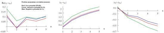
1. Introduction

The position and momentum of a quantum particle are intimately related and correlated, since knowledge of one precludes knowledge of the other. It is this correlation which gives rise to the Heisenberg uncertainty principle. In quantum mechanical formulism, the position operator does not commute with the momentum operator.

The momentum space wavefunction is the Dirac-Fourier transform (FT) of the position space one:

$$\varphi \left(p\right)=\frac{1}{{\left(2\pi \right)}^{1/2}}\int dx\psi \left(x\right)e^{-ipx}$$

(1)

This FT illustrates that each point in p-space is intertwined with every point in x-space, and vice versa.

One avenue of examining the correlations between x and p is to study it through statistical means [1,2,3,4,5,6,7]. To do this, one introduces a phase-space distribution that is dependent on both x and p. One example of such a distribution function is the Wigner function [8,9,10], defined as:

$$W(x,p)=\frac{1}{\pi }\int dy\psi (x+y){\psi }^{*}(x-y)e^{2ipy}$$

(2)

It has the attractive properties that its marginals are the x- and p-space densities, respectively, and it normalizes to unity:

$$\begin{array}{c}\hfill \int dpW(x,p)=\rho \left(x\right)={\left|\psi \left(x\right)\right|}^2\end{array}$$

$$\begin{array}{c}\hfill \int dxW(x,p)=\pi \left(p\right)={\left|\varphi \left(p\right)\right|}^2\end{array}$$

$$\begin{array}{c}\hfill \int dxdpW(x,p)=1\end{array}$$

(3)

On the other hand, it is a quasi-probability distribution, since it can attain negative values, which limits its interpretation as a true probability distribution in the conventional way.

The problem of determining the correlation between the position and momentum from Wigner functions has been addressed [11,12,13]. One can think of quantifying the correlation between the position and momentum variables by the use of tools taken from statistical theory. The usual manner of studying the correlation between two variables is through the use of the correlation coefficient [1,2,3,4,5,13] or through the use of mutual information from information theory [14]. Mutual information provides a more general measure of correlation, while the correlation coefficient captures linear dependencies.

Mutual information can be considered as a relative entropy or the distance of a distribution from the product of its marginals. It is defined in terms of the Wigner function as:

$$I_{xp}=\int dxdpW(x,p)ln\left[\frac{W(x,p)}{\rho \left(x\right)\pi \left(p\right)}\right]=s_{\rho }+s_{\pi }-s_w$$

(4)

where $s_{\rho }$, $s_{\pi }$ and $s_w$ are the Shannon entropies [15] of the position, momentum and Wigner distributions, respectively. These are defined as:

$$\begin{array}{c}\hfill s_{\rho }=-\int dx\rho \left(x\right)ln\rho \left(x\right)\end{array}$$

$$\begin{array}{c}\hfill s_{\pi }=-\int dp\pi \left(p\right)ln\pi \left(p\right)\end{array}$$

(5)

$$\begin{array}{c}\hfill s_w=-\int dxdpW(x,p)lnW(x,p)\end{array}$$

(6)

and are measures of the localization(delocalization) of the underlying distributions. Shannon entropies of other phase-space distributions have been discussed [16].

The interpretation of $I_{xp}$ as the difference between $s_{\rho }+s_{\pi }=s_t$ and $s_w$ is noteworthy, since $s_t$ forms the basis of the entropic uncertainty-like relationship [17]:

$$s_t=s_{\rho }+s_{\pi }\ge 1+ln\pi$$

(7)

whose lower bound corresponds to the ground-state harmonic oscillator. This entropy sum can be considered as the entropy of the separable phase-space distribution $\rho \left(x\right)\pi \left(p\right)$:

$$s_t=-\int dxdp\rho \left(x\right)\pi \left(p\right)ln\left[\rho \left(x\right)\pi \left(p\right)\right]$$

(8)

Another interpretation of $I_{xp}$ is that it is the entropic distance between the Wigner function of the system and a reference state, which is ground-state harmonic oscillator-like, since the Wigner function for the ground-state of the harmonic oscillator is separable and equal to the product of the position and momentum space densities.

The Wigner function can assume negative values. Thus, $s_w$ is a complex-valued quantity. It can be split into regions, where the Wigner function is positive (W${}^{+}$) and negative (W${}^{-}$):

$$\begin{array}{cc}{s}_w=& -\int dxdp{W}^{+}(x,p)\ln W^{+}(x,p)\hfill \\ & -\int dxdp{W}^{-}(x,p)\ln \left|W^{-}\right(x,p\left)\right|\hfill \\ & -i\pi \int dxdp{W}^{-}(x,p)\hfill \end{array}$$

(9)

It should be noted that the imaginary part of the entropy is proportional to the volume of the negative regions of the Wigner function, which have been related to entanglement [18] and with nonclassicality [19]. The presence of the negative regions in quasiprobability distributions has also been studied in connection with nonclassical effects [20,21]. Localization in phase-space and its relation with the uncertainty principle has been discussed [22,23,24,25,26].

The definition of the mutual information given above is also a complex-valued quantity, since it depends on $s_w$. Note also that it is not a mutual information in the strict sense, since the bound, $s_t-s_w\ge 0$, is not necessarily obeyed. We emphasize that the statistical correlation in this sense, as measured by $I_{xp}$, provides a measure of the difference between the Wigner function and a separable phase-space distribution [$\rho \left(x\right)\pi \left(p\right)$].

$I_{xp}$ has been applied to study position-momentum correlation in the particle-in-a-box model (PIAB) [6], where the mutual information was examined as a function of the quantum number. The PIAB model has an infinite potential at the edges of the box, so that the particle is confined inside the box. There is no potential inside the box. However, it would be interesting to examine the position-momentum correlation and localization (delocalization) of the Wigner function when the particle is under the influence of a potential. Does the statistical correlation between the position and momentum variables increase with the strength of the potential? Is this correlation, and the localization of the Wigner function, different for attractive potentials as compared to repulsive potentials?

2. The Quantum Corral Model

This model is a two-dimensional system of a particle confined to a circular hard-wall enclosure of radius unity and has been used to interpret experimentally realizable systems [27,28]. The natural co-ordinate system is polar co-ordinates with wavefunctions:

$${\psi }_{nk}(r,\varphi )=R_{nk}\left(r\right){\Phi }_k\left(\varphi \right)$$

(10)

where

$$R_{nk}\left(r\right)=\frac{2^{1/2}}{J_{\left|k\right|+1}\left(x_{nk}\right)}{J}_k\left(x_{nk}r\right)$$

(11)

$${\Phi }_k\left(\varphi \right)=\frac{1}{\sqrt{2\pi }}{e}^{ik\varphi }$$

(12)

and $n=1,2,3,\cdots ,\left|k\right|=0,1,2,3,\cdots$ . $J_k$ is a k-order Bessel function of the first kind, and $x_{nk}$ is the $n^{th}$ zero of this function. Information entropies in position and momentum space have been studied in this model [29,30].

One may obtain a radial Schrödinger equation by substituting the wave function in Equation (10) into the Schrödinger equation:

$$-\frac{1}{r}\frac{d}{dr}\left(r\frac{d{R}_{nk}}{dr}\right)+\frac{k^2}{r^2}{R}_{nk}=ϵR_{nk}$$

(13)

where $ϵ=\frac{2mE}{{\hslash }^2}$. Defining the new variable:

$$u_{nk}\left(r\right)=\sqrt{r}{R}_{nk}\left(r\right)$$

(14)

and substituting into Equation (13) gives:

$$-\frac{d^2{u}_{nk}}{d{r}^2}+\frac{k^2-1/4}{r^2}{u}_{nk}=ϵu_{nk}$$

(15)

This equation can be interpreted as a one-dimensional radial Schrödinger equation with effective potential given by:

$$\frac{k^2-1/4}{r^2}$$

(16)

Since the u’s are zero at $r=0$ and $r=1$, this model is equivalent to the particle-in-a-box model with unit length where the particle is now under the influence of an effective potential that is attractive towards the center of the confining region for $k=0$, while it is repulsive for all other integer values of k. This model provides the possibility of studying position-momentum correlation and the effect of the attractive and repulsive potentials. Results can also be compared and contrasted to those of the PIAB model [6].

The purpose of this work is the study of the position-momentum correlation in this radial model with effective potential to examine how the presence of an attractive or repulsive potential, and its intensity influences this correlation. The localization features of the Wigner function for the different potentials are also studied through the Shannon entropy and compared to the PIAB model with zero potential.

3. Results and Discussion

Wigner functions and their Shannon entropies were calculated by numerical Fourier transform of:

$$W_{nk}(r,p)=\frac{1}{\pi }\int dy{u}_{nk}(r+y)u_{nk}(r-y)e^{2ipy}$$

(17)

and numerical integration of Equation (6). $u_{nk}(r\pm y)$ are zero-valued outside of the interval $[0,1]$. This implies that $0\le r+y\le 1$ and $0\le r-y\le 1$. This leads to a restriction on the integration limits:

$$\begin{array}{cc}-r\le y\le +r,\hfill & \mathrm{if }0\le r\le \frac{1}{2}\hfill \\ -(1-r)\le y\le +(1-r),\hfill & \mathrm{if }\frac{1}{2}<r\le 1\hfill \end{array}$$

(18)

Entropies and mutual information are reported in units of $nats$. The numerical procedure was checked by numerically calculating Wigner functions of the PIAB model and comparing them to their known analytical expressions [31]. The normalization of the Wigner function was also verified.

3.1. Wigner Functions

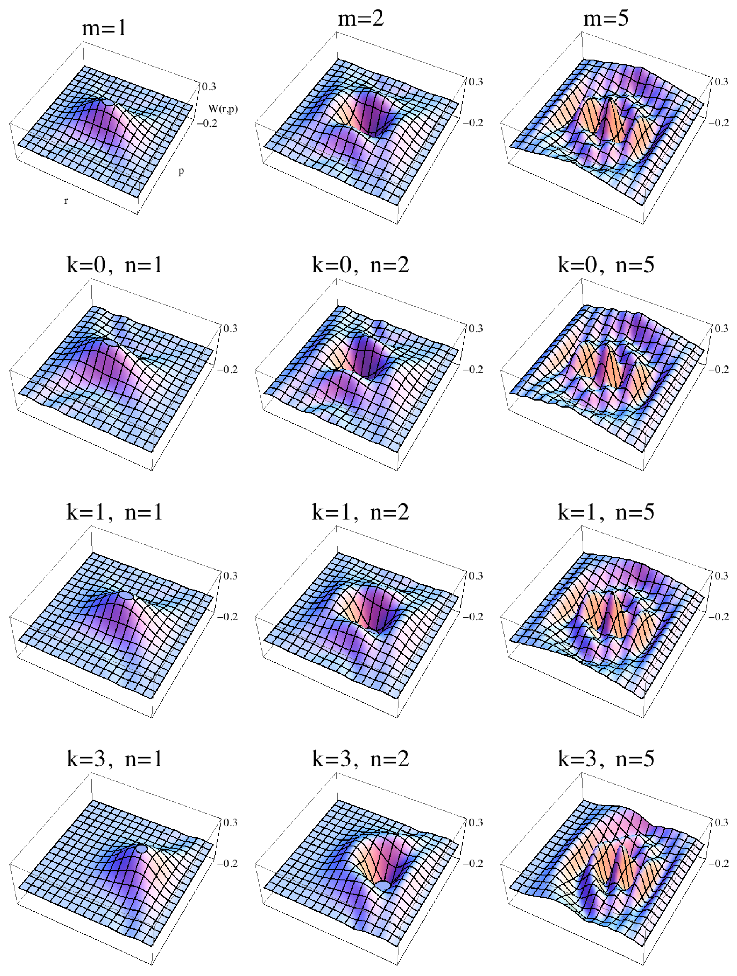
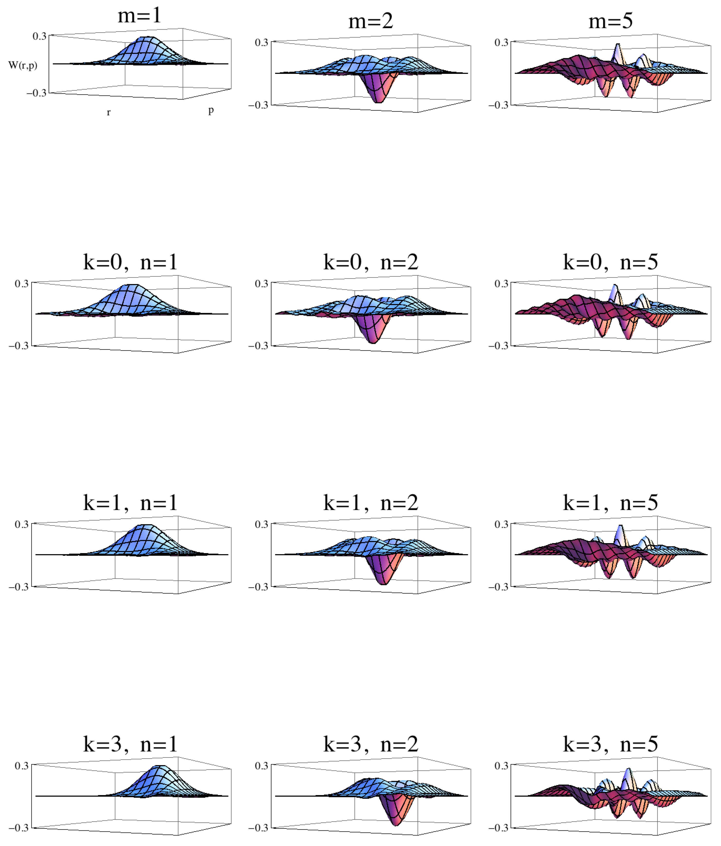
Figure 1 presents plots of the Wigner function of the PIAB model along with the radial model for attractive and repulsive potentials. The first row is the Wigner function of the PIAB model for quantum numbers $m=1,2,5$, while the other rows correspond to the effective potential model with $k=0,1,3$. Each row is plotted for quantum numbers, $n=1,2,5$. Thus, comparing the behavior of each row allows one insight into how the Wigner function is changing with excitation of the system (larger m or n). Comparing each column with its first entry (no potential) allows insight into how the Wigner function is affected by the presence of an attractive (second entry, $k=0$) or repulsive (third and fourth entries, $k=1,3$) potential.

Figure 1. Top-down perspective of plots of the Wigner function for the PIAB model (first row) and the radial model. Plots correspond to r-values between (0,1) and p-values between (−15,15).

Figure 1. Top-down perspective of plots of the Wigner function for the PIAB model (first row) and the radial model. Plots correspond to r-values between (0,1) and p-values between (−15,15).

One observes that all rows have similar characteristics. That is, the radial model is very similar to the PIAB one (first row) with slight differences. Going along each row, one sees the introduction of more nodal structure as the system is excited.

On comparing the first and second entries of each column, one appreciates that the second entries are slightly shifted towards the origin of $r=0$ due to the presence of the attractive potential. On the other hand, the third entry as compared to the first is displaced towards the right or the boundary at $r=1$ due to the presence of the repulsive potential. Comparing the last two entries of each column ($k=1,3$), one observes that a stronger repulsive potential shifts the Wigner function even more towards the boundary.

Figure 2 presents a sideways perspective where one can appreciate how the number of negative regions in the Wigner function increases with the excitation. The middle column ($n=2$) clearly shows that the negative region moves towards the origin with the introduction of the attractive potential while it is pushed towards the boundary with the repulsive one.

Figure 2. Sideways perspective of plots of the Wigner function for the position-momentum correlation in the particle-in-a-box model (PIAB) model (first row) and the radial model. Plots correspond to r-values between (0,1) and p-values between (−15,15).

Figure 2. Sideways perspective of plots of the Wigner function for the position-momentum correlation in the particle-in-a-box model (PIAB) model (first row) and the radial model. Plots correspond to r-values between (0,1) and p-values between (−15,15).

3.2. Shannon Entropy of the Wigner Function

Figure 3 shows $s_w$ as a function of quantum number n for $k=0,1$ and also for the PIAB model. Note that since $s_w$ is a complex-valued quantity, three different quantitative measures are used and plotted. Re[$s_w$], Im[$s_w$] and $|s_w|$ are all increasing functions of n and m and consistent in their behavior for all values of n and m. Of the three measures, Re[$s_w$] is the one that makes a lesser distinction between the different potentials, since the differences are very small.

Figure 3. Plots of the three measures of the Shannon entropy of the Wigner function and $s_t$ as a function of $n\left(m\right)$: $k=0$ (green), PIAB (red), $k=1$ (blue).

Figure 3. Plots of the three measures of the Shannon entropy of the Wigner function and $s_t$ as a function of $n\left(m\right)$: $k=0$ (green), PIAB (red), $k=1$ (blue).

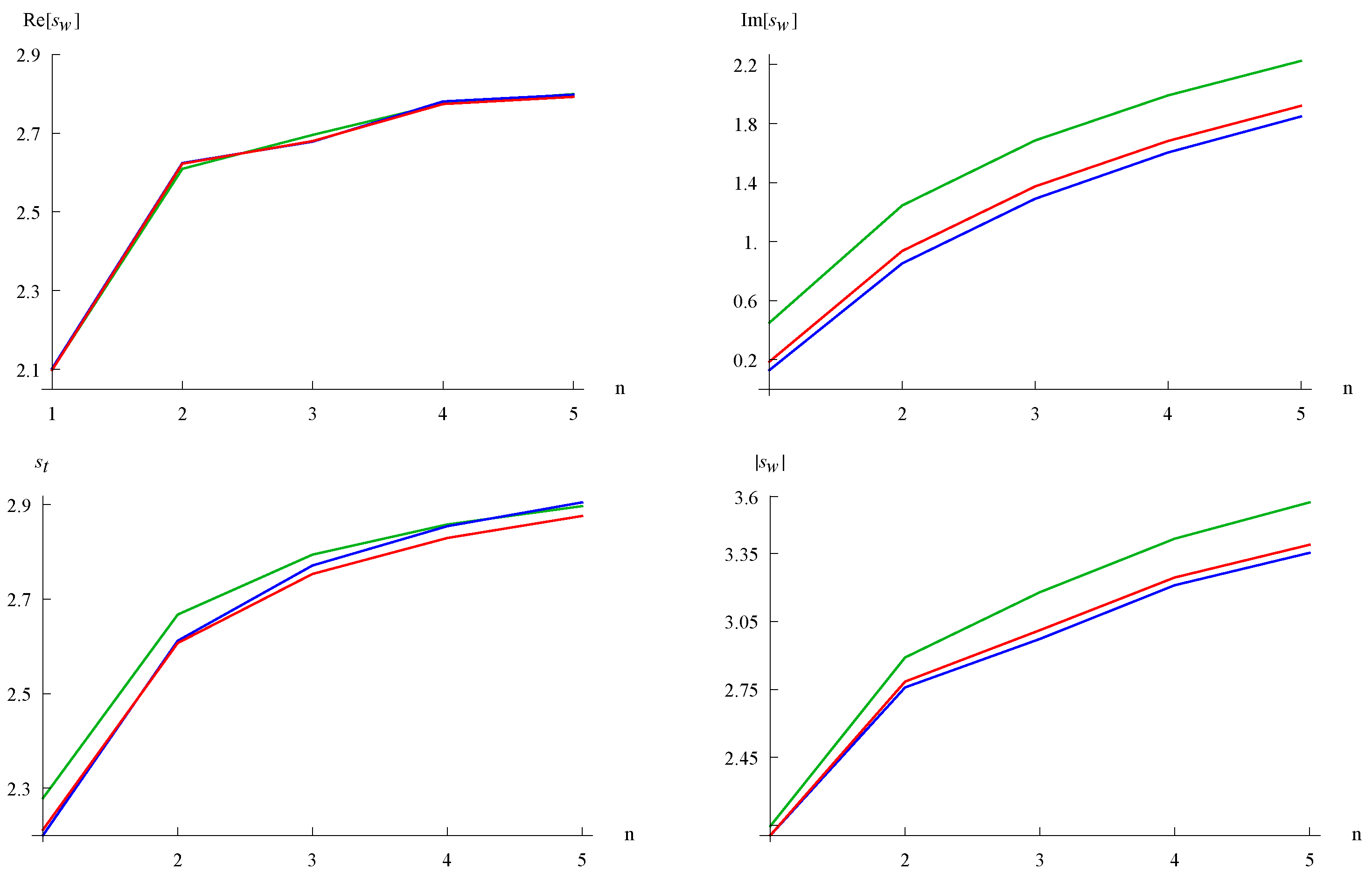
In the Im[$s_w$] and $|s_w|$ plots, the PIAB curve (zero potential) interpolates nicely between the $k=0$ (attractive potential) and $k=1$ (repulsive potential). The interpretation of these plots is that the Wigner function delocalizes with increasing n. This behavior was also noted for $k=3,5$.

The result that the Im[$s_w$] curve increases with n illustrates that the negative regions of the Wigner function become larger as n increases. Also, one sees that the volume of the negative region in PIAB is between that of $k=0$ and $k=1$, as stated in the previous paragraph.

Furthermore, the ordering of the $k=0$, PIAB and $k=1$ curves in the Im[$s_w$] and $|s_w|$ plots is maintained for all values of n. That is, the presence of an attractive potential increases the volume of the negative regions (comparing the $k=0$ curve to the PIAB one), while the repulsive potential decreases the volume (comparing the $k=1$ curve to the PIAB one). The interpretation is that the attractive potential delocalizes the distribution, while the repulsive one localizes the distribution, with respect to the case of no potential (PIAB).

The $s_t$ plots are also presented in Figure 3. These correspond to the Shannon entropies of a separable phase-space distribution and can be compared to the other measures. All values of $s_t$ obey the entropic uncertainty relationship. Important to note is that while the behavior of $s_t$ is similar to the other measures, it does not preserve the ordering of the $k=0$, PIAB and $k=1$ curves as does Im[$s_w$] and $|s_w|$. That is, there are points where the curves crossover (similar to Re[$s_w$]). The observation here is that measures that incorporate the negative regions of the Wigner function respect the relative ordering, while the $s_t$ measure that comes from a separable and non-negative phase-space distribution does not.

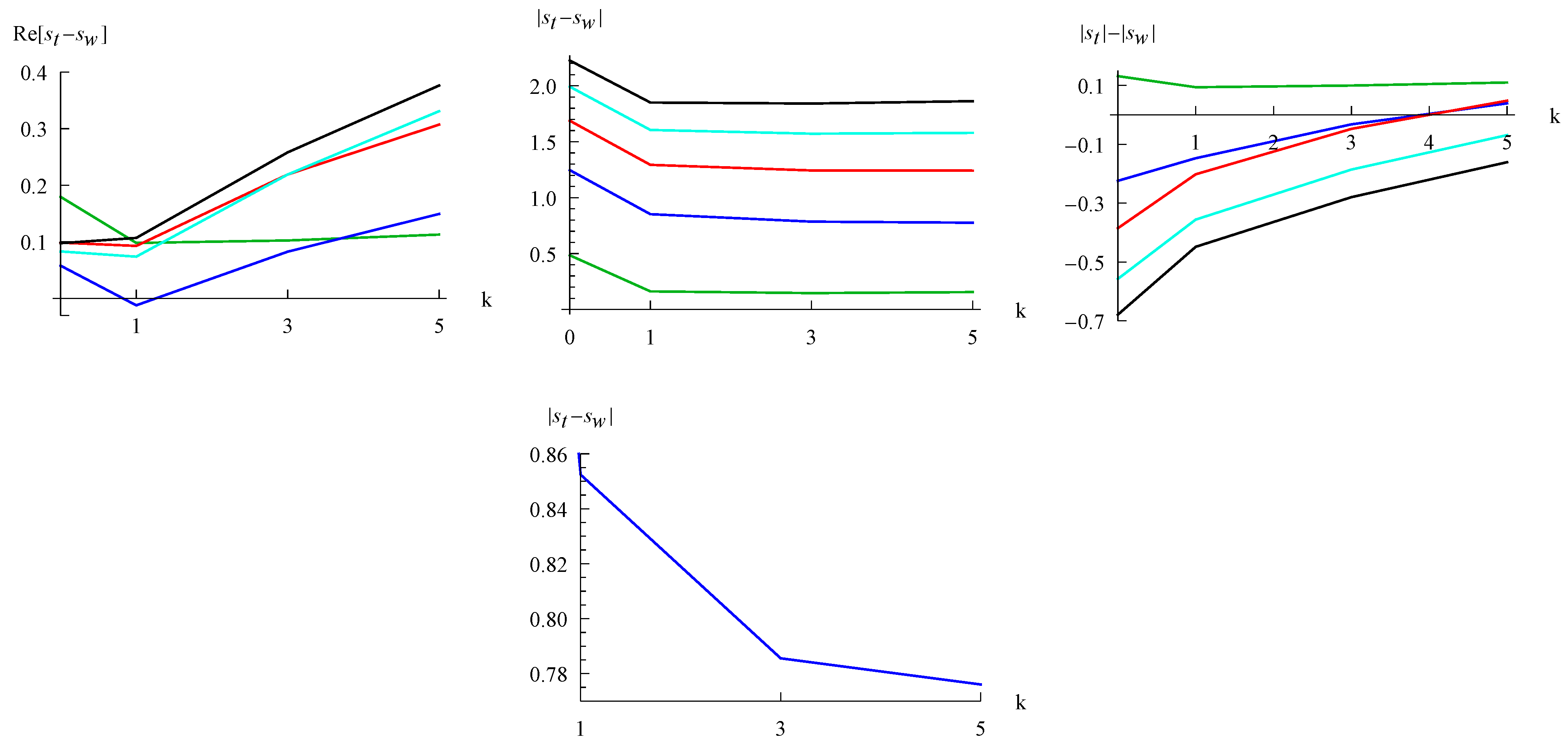
Figure 4 plots the three measures as a function of k. Re[$s_w$] does not vary much with k. On the other hand, Im[$s_w$], and to a lesser extent $|s_w|$, clearly show the change in the shape of the curve on going from $k=0$ to $k>0$. Thus, the difference between the attractive and repulsive potentials manifests itself in the imaginary part of $s_w$ (which is also included in $|s_w|$).

Figure 4. Plots of the three measures of the Shannon entropy of the Wigner function as a function of k: $n=1$ (green), $n=2$ (blue), $n=3$ (red), $n=4$ (light blue), $n=5$ (black). The bottom curves are an enhanced scale for $n=2$ with repulsive potentials $k\ge 1$.

Figure 4. Plots of the three measures of the Shannon entropy of the Wigner function as a function of k: $n=1$ (green), $n=2$ (blue), $n=3$ (red), $n=4$ (light blue), $n=5$ (black). The bottom curves are an enhanced scale for $n=2$ with repulsive potentials $k\ge 1$.

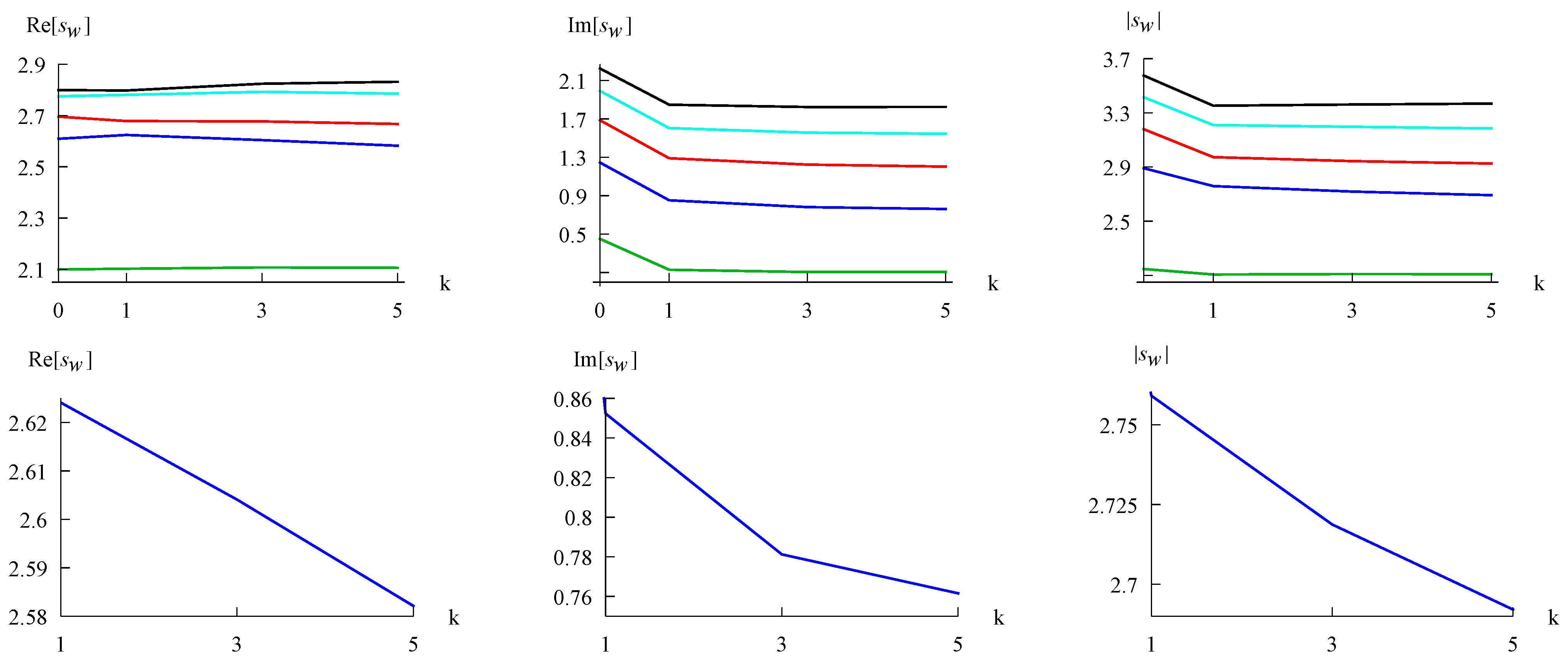
Both the Im[$s_w$] and $|s_w|$ curves are somewhat flat for $k\ge 1$. This suggests that the strength or intensity of the repulsive potential is not a dominant factor in the volume of the negative regions and in the localization as a whole. This behavior can be interpreted by returning to the Wigner function plots in Figure 1. Take, for example, the last two entries of the first column, which are perhaps the clearest. The stronger repulsive potential in the last entry compresses the Wigner function toward the boundary in the r direction. This compression results in a broadening of the function in the p direction, due to the uncertainty principle. Thus, there is a small net change in the localization.

The last row of Figure 4 plots the $n=2$ curve for each quantity using an enhanced scale. One observes that all quantities decrease with increasing k (stronger repulsive potentials). We stress that the trend presented for $n=2$ is a generalized one which was observed for several groups of n. There are, however, $n^{\prime }s$, where the trend is increasing, e.g., $n=5$ in Re[$s_w$] and $|s_w|$. Such an increasing trend was also observed for $s_t$ [30].

3.3. Mutual Information

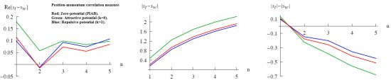
Figure 5 plots the three measures of mutual information, Re[$s_t-s_w$], $|s_t-s_w|$ and $|s_t|-|s_w|$, as a function of n for $k=0$, PIAB and $k=1$. Important to note is that the behavior is similar to PIAB in all three cases. For the latter two measures, which incorporate the imaginary parts, the interpretation is that the position-momentum correlation increases in magnitude with n as in the PIAB model. Also, the PIAB curve interpolates nicely between the $k=0$ and $k=1$ curves. For the Re[$s_t-s_w$] curves, the interpretation is less transparent as the curves increase and decrease.

Figure 5. Plots of the three measures of the mutual information as a function of $n\left(m\right)$: $k=0$ (green), PIAB (red), $k=1$ (blue).

Figure 5. Plots of the three measures of the mutual information as a function of $n\left(m\right)$: $k=0$ (green), PIAB (red), $k=1$ (blue).

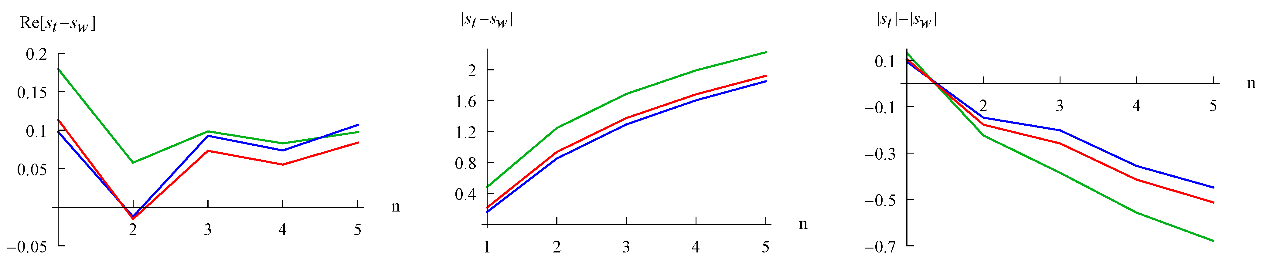
In the latter two plots, the magnitude of the correlation is greater for the $k=0$ curve as compared to the PIAB one. Thus, the attractive potential increases the magnitude of the position-momentum correlation. On the other hand, the magnitude of the correlation is smaller for the $k=1$ curve as compared to PIAB. Hence, the repulsive potential decreases the magnitude of the position-momentum correlation.

The imaginary component of $I_{rp}$, Im[$s_t-s_w$] can also be considered as a correlation measure. It is -Im[$s_w]$ and is minus the curve presented in Figure 3. Examining this curve, the interpretation would be that the magnitude of the correlation increases with n. It would also be consistent with $|s_t-s_w|$ and $|s_t|-|s_w|$ in the interpretation of the effects of the potentials on the magnitude of the correlation.

Figure 6. Plots of the three measures of the mutual information as a function of k: $n=1$ (green), $n=2$ (blue), $n=3$ (red), $n=4$ (light blue), $n=5$ (black). The bottom curve for $|s_t-s_w|$ is an enhanced scale for $n=2$ with repulsive potentials, $k\ge 1$.

Figure 6. Plots of the three measures of the mutual information as a function of k: $n=1$ (green), $n=2$ (blue), $n=3$ (red), $n=4$ (light blue), $n=5$ (black). The bottom curve for $|s_t-s_w|$ is an enhanced scale for $n=2$ with repulsive potentials, $k\ge 1$.

Figure 6 presents the curves as a function of k. All curves show a distinction between attractive and repulsive potentials. The interpretation is that the magnitude of the correlation is greater for attractive potentials than for repulsive ones. Differences are that in $|s_t-s_w|$ the position-momentum correlation is not greatly affected by the strength of the repulsive potential ($k\ge 1$), while for the other measures, the interpretation is that the magnitude of the correlation increases (Re[$s_t-s_w$]) or decreases ($|s_t|-|s_w|$) with the intensity of the potential.

The $|s_t-s_w|$ curve for $n=2$ is presented below with an enhanced scale. On this scale, it shows that $|s_t-s_w|$ decreases, thus the correlation decreases with the intensity of the repulsive potential. This is similar to the behavior of the $|s_t|-|s_w|$ curves. These results for $n=2$ also hold for the $n=3$ points, but not for the others. On the other hand, a decrease from $k=1$ to $k=3$ was observed for all the studied values of $n^{\prime }s$.

4. Conclusions

Solutions to the radial Schrödinger equation of a particle in a quantum corral are used to study the effects of an attractive or repulsive effective potential on the behavior of the respective Wigner functions. The localization/delocalization in the Wigner function is studied by its Shannon entropy. We show that the entropy increases as a function of quantum number n for both attractive and repulsive potentials, similar to the case of zero potential [particle-in-a-box (PIAB)]. The imaginary part of the entropy increases with n, which illustrates that the volume of the negative regions of the Wigner function increases with n. Furthermore, the PIAB curve (zero potential) interpolates between the attractive ($k=0$) and repulsive ($k=1$) potentials. The interpretation is that the attractive potential increases the negative volume of the Wigner function, while the repulsive potential decreases this volume. A study of the Shannon entropy versus k highlights that the entropy detects the difference between attractive and repulsive potentials. Mutual information, defined as the difference between the sum of position and momentum space entropies and the Shannon entropy of the Wigner function, is used to study the correlation between position and momentum. This correlation increases with n and is consistent with that in the particle-in-a-box model. Moreover, the values of the PIAB model interpolates between the $k=0$ and $k=1$ cases. The presence of an attractive potential increases the magnitude of this correlation, while a repulsive one decreases this correlation. As a function of k, the results show a clear distinction between attractive and repulsive potentials. The magnitude of the correlation is observed to decrease with the strength of the repulsive potential. The importance of the imaginary components of the information measures, corresponding to the volume of the negative regions of the Wigner function, is emphasized.

References

- Lévy-Leblond, J.-M. Correlation of quantum properties and the generalized Heisenberg inequality. Am. J. Phys. 1986, 54, 135–136. [Google Scholar] [CrossRef]
- De la Torre, A.C.; Iguain, J.L. Manifest and concealed correlations in quantum mechanics. Eur. J. Phys. 1998, 19, 563–568. [Google Scholar] [CrossRef]
- Campos, R.A. Correlation coefficient for incompatible observables of the quantum harmonic oscillator. Am. J. Phys. 1998, 66, 712–718. [Google Scholar] [CrossRef]
- Campos, R.A. Wigner quasiprobability distribution for quantum superpositions of coherent states, a Comment on “Correlation coefficient for incompatible observables of the quantum harmonic oscillator" [Am. J. Phys. 66 (8), 712-718 (1998)]. Am. J. Phys. 1999, 67, 641–642. [Google Scholar] [CrossRef]
- Campos, R.A. Quantum correlation coefficient for position and momentum. J. Mod. Opt. 1999, 46, 1277–1294. [Google Scholar] [CrossRef]
- Laguna, H.G.; Sagar, R.P. Shannon entropy of the Wigner function and position-momentum correlation in model systems. Int. J. Quantum Inf. 2010, 8, 1089–1100. [Google Scholar] [CrossRef]
- Laguna, H.G.; Sagar, R.P. Position-momentum correlations in the Moshinsky atom. J. Phys. A Math. Theor. 2012, 45, 025307. [Google Scholar] [CrossRef]
- Wigner, E.P. On the quantum correction for thermodynamic equilibrium. Phys. Rev. 1932, 40, 749–759. [Google Scholar] [CrossRef]
- Hillery, M.; O’Connell, R.F.; Scully, M.O.; Wigner, E.P. Distribution-functions in physics-fundamentals. Phys. Rep. 1984, 106, 121–167. [Google Scholar] [CrossRef]
- Tatarskii, V.I. The Wigner representation of quantum mechanics. Usp. Fiz. Nauk. 1983, 139, 587–619. [Google Scholar] [CrossRef]
- Halliwell, J.J. Correlations in the wave-function of the universe. Phys. Rev. D 1987, 36, 3626–3640. [Google Scholar] [CrossRef]
- Anderson, A. On predicting correlations from Wigner functions. Phys. Rev. D 1990, 42, 585–589. [Google Scholar] [CrossRef]
- Robinett, R.W.; Doncheski, M.A.; Bassett, L.C. Simple examples of position-momentum correlated Gaussian free-particle wave packets in one dimension with the general form of the time-dependent spread in position. Found. Phys. Lett. 2005, 18, 455–475. [Google Scholar] [CrossRef]
- Cover, T.M.; Thomas, J.A. Elements of Information Theory; John Wiley and Sons: New York, NY, USA, 1991; p. 251. [Google Scholar]
- Shannon, C.E. A mathematical theory of communication. Bell Syst. Tech. J. 1948, 27, 379–423. [Google Scholar] [CrossRef]
- Wehrl, A. General properties of entropy. Rev. Mod. Phys. 1978, 50, 221–260. [Google Scholar] [CrossRef]
- Bialynicki-Birula, I.; Mycielski, J. Uncertainty relations for information entropy in wave mechanics. Commun. Math. Phys. 1975, 44, 129–132. [Google Scholar] [CrossRef]
- Dahl, J.P.; Mack, H.; Wolf, A.; Schleich, W.P. Entanglement versus negative domains of Wigner functions. Phys. Rev. A 2006, 74, 042323. [Google Scholar] [CrossRef]
- Kenfack, A.; Życzkowski, K. Negativity of the Wigner function as an indicator of non-classicality. J. Opt. B Quantum Semiclass. Opt. 2004, 6, 396–404. [Google Scholar] [CrossRef]
- Lütkenhaus, N.; Barnett, S.M. Nonclassical effects in phase-space. Phys. Rev. A 1995, 51, 3340–3342. [Google Scholar] [CrossRef] [PubMed]
- Sperling, J.; Vogel, W. Representation of entanglement by negative quasi-probabilities. Phys. Rev. A 2009, 79, 042337. [Google Scholar] [CrossRef]
- Mirbach, B.; Korsch, H.J. A generalized entropy measuring quantum localization. Ann. Phys. 1998, 265, 80–97. [Google Scholar] [CrossRef]
- Gnutzmann, S.; Życzkowski, K. Renyi-Wehrl entropies as measures of localization in phase space. J. Phys. A Math. Gen. 2001, 34, 10123–10139. [Google Scholar] [CrossRef]
- Pennini, F.; Plastino, A. Localization estimation and global vs. local information measures. Phys. Lett. A 2007, 365, 263–267. [Google Scholar] [CrossRef]
- Pennini, F.; Plastino, A.; Ferri, G.L.; Olivares, F. Semiclassical localization and uncertainty principle. Phys. Lett. A 2008, 372, 4870–4873. [Google Scholar] [CrossRef]
- Olivares, F.; Pennini, F.; Ferri, G.L.; Plastino, A. Note on semiclassical uncertainty relations. Braz. J. Phys. 2009, 39, 503–506. [Google Scholar] [CrossRef]
- Crommie, M.F.; Lutz, C.P.; Eigler, D.M. Confinement of electrons to quantum corrals on a metal-surface. Science 1993, 262, 218–220. [Google Scholar] [CrossRef] [PubMed]
- Crommie, M.F.; Lutz, C.P.; Eigler, D.M. Imaging standing waves in a 2-dimensional electron-gas. Nature 1993, 363, 524–527. [Google Scholar] [CrossRef]
- Dehesa, J.S.; Martínez-Finkelshtein, A.; Sorokin, V.N. Short-wave asymptotics of the information entropy of a circular membrane. Int. J. Bifurcation Chaos 2002, 12, 2387–2392. [Google Scholar] [CrossRef]
- Corzo, H.H.; Castaño, E.; Laguna, H.G.; Sagar, R.P. Measuring localization-delocalization phenomena in a quantum corral. J. Math. Chem. 2013, 51, 179–193. [Google Scholar] [CrossRef]
- Belloni, M.; Doncheski, M.A.; Robinett, R.W. Wigner quasi-probability distribution for the infinite square well: Energy eigenstates and time-dependent wave packets. Am. J. Phys. 2004, 72, 1183–1192. [Google Scholar] [CrossRef]
© 2013 by the authors; licensee MDPI, Basel, Switzerland. This article is an open access article distributed under the terms and conditions of the Creative Commons Attribution license (http://creativecommons.org/licenses/by/3.0/).
Share and Cite
MDPI and ACS Style
Laguna, H.G.; Sagar, R.P. Phase-Space Position-Momentum Correlation and Potentials. Entropy 2013, 15, 1516-1527. https://doi.org/10.3390/e15051516
AMA Style
Laguna HG, Sagar RP. Phase-Space Position-Momentum Correlation and Potentials. Entropy. 2013; 15(5):1516-1527. https://doi.org/10.3390/e15051516
Chicago/Turabian StyleLaguna, Humberto G., and Robin P. Sagar. 2013. "Phase-Space Position-Momentum Correlation and Potentials" Entropy 15, no. 5: 1516-1527. https://doi.org/10.3390/e15051516