1. Introduction
Studies in (computational) learning theory mostly tend to concentrate on situations where potentially ever increasing number of training examples is available. While such results can lead to deep insights into the workings of learning algorithms, e.g., linking together characteristics of the data generating distributions, learning machines and sample sizes, there can be situations where, by very nature of the problem, only extremely small samples are available. In such situations it is of utmost importance to theoretically analyze exactly what and under what circumstances can be learnt. One example of such a scenario in count data is detection of differentially expressed genes, where even subtle changes in gene expression levels can be indicators of biologically crucial processes [
1]. When replicas are costly to obtain one can attempt to use the limited data at one’s disposal to make the relevant inferences, as for example in the Audic and Claverie approach [
2,
3,
4,
5,
6]. Another situation where available count data can be extremely sparse is estimation of time delay in non-stationary gravitationally lensed photon streams. When the scale of variability of the source is of order, say, of more than tens of days and observation gaps are not too long, one can resolve the time delay between lensed images of the same source by working directly with daily measurements of fluxes in the radio, optical or X-ray range [
7,
8,
9,
10]. However, when the variability scale is of the order of hours, one must turn to photon streams in the lensed images. One possibility of time delay detection in such cases is through comparing counts in relatively short and time-shifted moving time windows in the lensed photon streams.
In this paper we theoretically study what happens in the extreme situation of unreplicated data when the inference has to be performed on the smallest sample possible—sample of size 1. We consider a model-based Bayesian approach that averages over possible Poisson models with weighting determined by the posterior over the models, given the single observation. In fact, such a Bayesian approach has been considered in the bioinformatics literature under the assumption of flat improper prior over the Poisson rate parameter [
2,
3,
4,
5,
6]. One can, of course, be excused for being highly sceptical about the relevance of such inferences, yet the methodology has apparently been used in a number of successful studies. In an attempt to build theoretical foundations behind such inference schemes, we proved a rather surprising result [
11]: The expected Kullback–Leibler divergence from the true unknown Poisson distribution to its
model learnt from a single realization never exceeds 1/2 bit.
Even though the field of bioinformatics is moving fast and better procedures for detection of differentially expressed genes have been introduced (e.g., not relying on the Poisson assumption, specifically taking into account potential dependencies among the genes,
etc.), the primary focus of this study is different. Irrespective of the application domain, we theoretically investigate how reliably can a model for count data be build from a single count observation, under the assumption of a Poisson source. There are two issues that need careful consideration:
Equal a-priori weighting (flat prior) over possible (unknown) Poisson sources is unrealistic. Typical values of observed counts are usually bounded by the nature of the problem (e.g., gene magnification setting used in the experiments or time window on the photon streams). One may have a good initial (a-priori) guess as to what ranges of typical observed counts might be reasonably expected. In particular, we are interested in the low count regimes. In such cases, it is desirable to incorporate such prior knowledge into the inference mechanism. In this study, we do this in the Bayesian framework through prior distribution over the expected counts.
To understand potential benefits of the proposed learning/inference method (in our case Bayesian approach), it is important to compare it with a simple straightforward baseline (here maximum likelihood estimation). We contrast the expected Kullback–Leibler divergences from the true unknown Poisson distribution to its Bayesian and maximum likelihood estimates, inferred from a single realization.
The paper has the following organization. In
Section 2 we introduce the maximum likelihood and Bayesian (with flat prior over mean rates) approaches to inferring predictive distribution over counts based on a single count observation. We also briefly review past work on information theoretic properties of the two approaches.
Section 3 contains derivation of a more general Bayesian approach with gamma prior on the mean count parameter. In
Section 4 we calculate the first two central moments of our generalized model. This enables us to better understand the influence of the prior on the inferred model and highlight the differences with the previous approach using the flat (improper) prior. In
Section 5 we perform an information theoretic study of learning capabilities of the generalized model. Empirical investigations are presented in
Section 6 and the main findings are discussed and summarized in
Section 7.
3. Generalized with Gamma Prior
In this section we will generalize
through the use of (conjugate) gamma prior
on the Poisson mean parameter
λ. The positive parameters
determine the overall shape of the prior. Given a single observation
x, the posterior
is the gamma distribution with parameters
and
,
The mean of
is equal to
. A loose intuitive interpretation of the prior parameters
(assuming they are integers) is that prior to seeing the current data (in our case only one observation (count)
x), we have seen
β “observations”,
, with the total cumulative count
. Hence the mean parameter estimate would shift from
x (ML estimation corresponding to
) to
.
As in the case of
, having observed a count
x, we build a predictive distribution over future counts
y by integrating out the mean parameter
λ with respect to the posterior
,
From normalization of the gamma distribution we get
and so
leading to
It can be easily verified that the original is obtained as a special case of when and . If Jeffrey’s prior were used instead of the flat prior in , we would obtain with and etc.
If
α is an integer, we have
where
is the observed count including prior observations. This expression generalizes
(5),
While
(9) can be used with any appropriate setting of
(e.g., given a prior knowledge of the range of counts one may reasonably expect), in this contribution we concentrate on using the gamma prior to mitigate for the unrealistic equal weighting of all
in the flat prior behind
. Indeed, the observed counts are typically bounded by the nature of the problem and one can represent this through setting
and varying
in the gamma prior
underlying
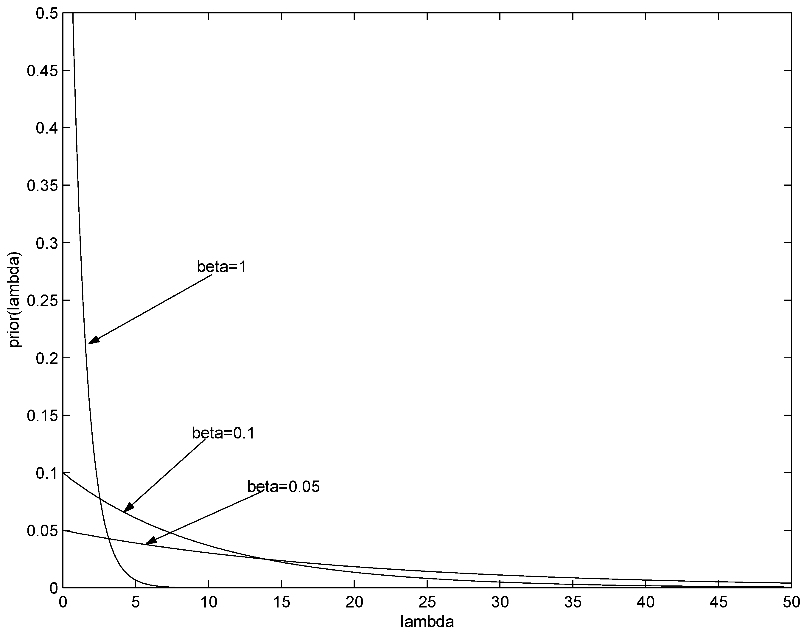
. Some examples of such priors are shown in
Figure 2. Decreasing
β leads to weaker emphasis on low
λ, eventually recovering the flat (improper) prior for
.
Figure 2.
Gamma prior . Shown are the priors for three possible values of parameter β, .
Figure 2.
Gamma prior . Shown are the priors for three possible values of parameter β, .
In
Section 2.3 maximum likelihood estimation was regularized at zero count by imposing a non-zero “count”
ϵ instead of the observed zero one. The generalized form of
,
can be also viewed as an alternative “soft” form of regularization of the maximum likelihood approach at zero counts.
Parameter
β in the Gamma prior
can be set in a data driven manner, e.g., using the following strategy: Given the observed count
x, we require that the area up to
covered by the prior is equal to
θ, for some threshold
(e.g.,
). In other words,
, where
is the cumulative distribution function of
. This leads to
For zero observed count , and the prior gets more concentrated on smaller values of λ as likely candidates for the mean count of the underlying Poisson source. With increasing count values the parameter decreases to 0 and the prior gradually approaches the flat prior of .
Finally, we contrast
with the negative binomial distribution
with parameters
and
. One interpretation of the negative binomial distribution
is that it corresponds to a Gamma–Poisson mixture that one obtains by imposing a Gamma prior
on the mean count parameter
λ of the Poisson distribution
and integrating out
λ. In our context it is natural to identify
r and
with hyperparameters
α and
β used in
. It follows that
. Hence, we rewrite Equation (
12) as
Direct comparison of (13) with (9) leads to an intuitive insight: The
β prior measurements of total count
α introduced by the gamma prior
are in the case of
extended with a single observation
x, resulting in
observations of total count
. This can be represented by
It follows that
Bayesian averaging in
with respect to the posterior over
λ, given a count
x, differs from the corresponding negative binomial distribution
by the factor
that depends on the difference between the prior+observed count
and
y.
4. First and Second Moments of the Generalized
In [
11] we showed that
and the underlying Poisson distribution are quite similar in their nature: for any (integer) mean rate
, the Poisson distribution
has two neighboring modes located at
λ and
, with
. Analogously, given a count
,
has two neighboring modes, one located at
x, the other at
, with
. As in Poisson distribution, the values of
decrease as one moves away from the modes in both directions. In this section we derive the first two moments of the generalized
,
. As a special case, we will show that as a result of Bayesian averaging, the variance of
is double that of the underlying (unobserved) Poisson distribution.
Theorem 3 Consider a non-negative integer x and the associated generalized model . Then, Proof: Let us evaluate
In the third equality we have used substitution
and the last equality follows from
. By (15),
For the variance of
we have
Now,
Using (16), (18) and (20), we obtain
which can be solved as
Plugging (22) into (19) we obtain
☐
Given an observation
x, the maximum likelihood estimate of the underlying Poisson distribution is the Poisson distribution with mean
x,
After observing
x, the mean of the maximum likelihood and
estimates is
x and
, respectively. Hence, Bayesian averaging in
induced by the flat improper prior over the mean rate
λ results in increased expected value
of the next count from the same underlying source, given that the current count
x. However, a much more marked consequence of using the flat prior can be seen in the variance of
: while variance of the maximum likelihood is
x, it is
in
.
Theorem 3 illustrates the role of more concentrated prior over λ on the generalized model. The mean expected count, after seeing x, is equal to the mean of the posterior over λ, namely . As explained earlier, observed single count x with prior β counts of cumulative value α results in counts of cumulative value . Hence the mean count per observation is . As with Poisson distribution, the variance of the generalized model is closely related to its mean and approaches the mean with increasing number of prior counts β.
As for the soft regularization , its mean is, as expected, biased towards values smaller than the observed count x, provided . Increased values of β result in smaller variance of . But how do such prior parameter modifications manifest themselves in terms of accuracy of estimation of the underlying source? This question is investigated in the next section.
5. Expected Divergence of the Generalized from the True Underlying Poisson Distribution
Consider an underlying Poisson source
generating counts
x. In this section we would like to quantify the average divergence
of the corresponding generalized
,
(“softly” regularized ML), from the truth
, if we repeatedly generated a “representative” count
x from
. The same question was considered in the context of maximum likelihood estimation in
Section 2.3. In particular, we are interested in specifying under what circumstances is the generalized form of
,
, preferable to the original
and how it fares with the maximum likelihood estimation
of
Section 2.3.
Theorem 4 Consider an underlying Poisson distribution parameterized by some . Then for ,A higher order approximation (up to order ) reads: Proof: Let us first express the divergence
. We have
where
is the entropy of the source
and
Denoting (for integer
)
by
, we write
We are now ready to calculate the expectation
.
We have proved in [
11] that
, and so
Using entropy approximation (see [
11]), one obtains
leading to (in log base 2)
Finally,
which is equivalent to (
24).
The higher order expression (
25) is simply obtained by using higher order approximation to
.
☐
Note that for
we recover our original result [
11] that the expected divergence
of the original
from the “truth”
is (up to terms of order
never greater than 1/2 bit. The soft regularization in
(using prior
with
) can result in larger expected divergence from the underlying source than is the case for
(using improper flat prior over
λ). Moreover, (unlike in
) such a regularization causes linear divergence of
for large
λ. The next theorem specifies for which underlying Poisson sources the soft regularization approach of
is preferable to the original
.
Theorem 5 For Poisson sources with mean ratesit holds and hence is on average guaranteed to approximate (in the Kullback–Leibler divergence sense) the underlying source better than the original . Proof: It was shown in [
11] that for the original
,
From (27) and (29) we have that the difference between the expected divergences of the original and generalized forms of
is
The result follows from solving for
.
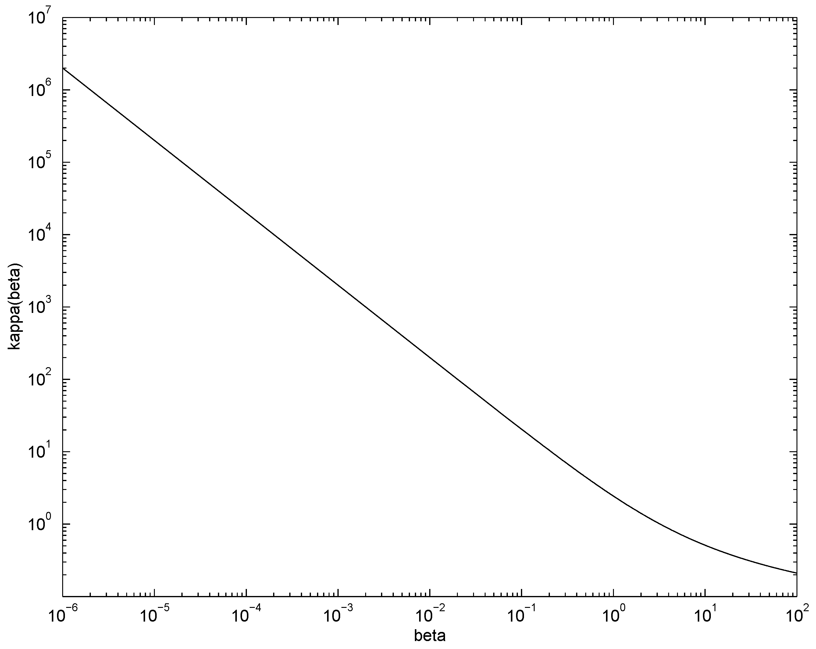
The graph (in log-log scale) of
is shown in
Figure 3. An alternative way of data-driven setting of parameter
β is suggested by the fact that
is lower bounded by
. If the experimental setting is such that most counts are expected not to exceed some
,
β can be set to
, so that
is preferable to
.
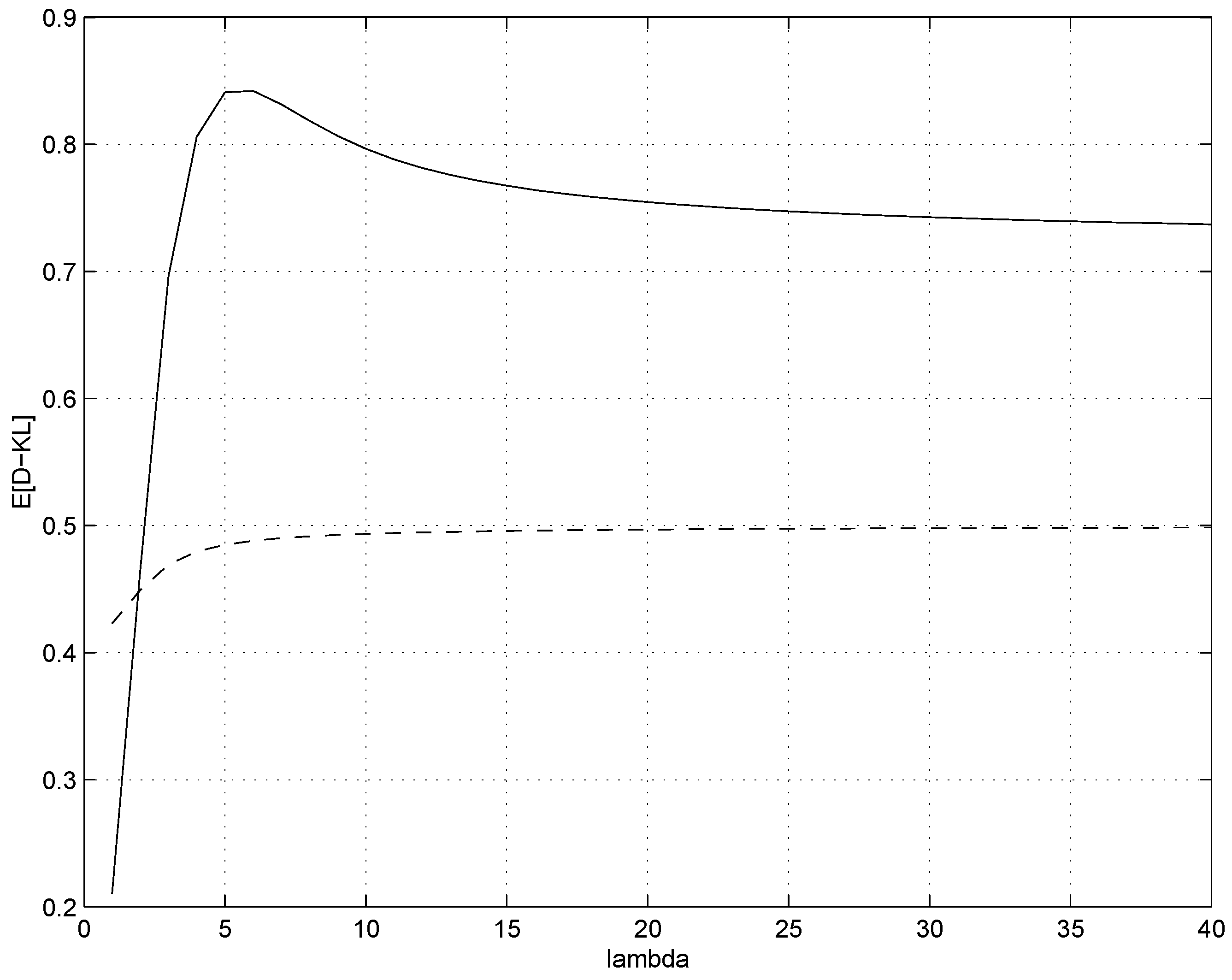
In
Figure 4 we present the expected divergences
(solid line) and
(dashed line) for
(left) and
(right). As expected, for underlying sources with small mean counts
λ the advantage of using the regularized form
(as opposed to the original
) is more pronounced. However, for larger
λ there is a heavy price to be paid in terms of inaccurate modelling by
.
Figure 3.
Graph of . For Poisson sources with mean rates , and hence is on average guaranteed to approximate the underlying source better than the original .
Figure 3.
Graph of . For Poisson sources with mean rates , and hence is on average guaranteed to approximate the underlying source better than the original .
Figure 4.
Expected divergences (solid line) and (dashed line) for (left) and (right).
Figure 4.
Expected divergences (solid line) and (dashed line) for (left) and (right).
6. Empirical Investigations
To investigate potential value of the more sophisticated Bayesian approach in the original and the generalized Audic–Claverie frameworks (
Section 2.1 and
Section 3, respectively) against the baseline of simple (regularized) maximum likelihood estimation (
Section 2.3), we conducted a series of simple illustrative experiments. In the generalized Audic–Claverie framework developed in this study, we used the two schemes for setting the regularization parameter
β suggested in
Section 3 and
Section 5. In the regularized maximum likelihood approach
we set
. From
Figure 1, it appears that the biggest difference between the expected divergences from the true underlying Poisson source
to the original
and the maximum likelihood estimate occurs for small mean rates
λ roughly around
. We therefore run the experiments with
.
For illustration purposes, we follow the data generation mechanism used in [
13] to compare methods for distinguishing between differential expression of genes associated with two treatment regimes. We stress that in no way we suggest that our experiments have strong relevance for bioinformatics, nor do we claim that the framework of [
13] is the best test bed for assessing differential gene expression detection algorithms. We use the framework of [
13] merely to illustrate whether the sophistication of the Bayesian approach (as opposed to simple (regularized) maximum likelihood) can bring benefits in a practical situation with low-count data.
Gene counts are simulated across the two treatment groups
and
. The tests are assessed by comparing false positive and true positive rates. In each experiment 10,000 gene pair counts
,
, were produced, counts
and
associated with regimes
and
, respectively. As specified above, the sampling rate for
was fixed at
throughout the experiment. We varied the mean
fold change (LFC) between
and
from −2 to 2. Each gene pair count
,
, was obtained through a generative process specified in [
13] and described in detail in
Appendix A.
Having generated the gene pair counts, we used methods considered in this study to make a decision for each , whether the counts originated from the same underlying source, i.e., whether when generating and , the mean rates in the two regimes and were identical (). Given the “test distribution” and a confidence level , we guess that originated from the same source if the -quantile around the mean of contains and vice-versa, i.e., if the -quantile around the mean of contains . In place of we used , its regularized form and the regularized maximum likelihood estimate with .
For a given confidence level and test statistic we calculate the false positive rate (type I error rate) as the proportion of times a gene count pair was declared to have originated from two different underlying sources (differentially expressed gene) when in fact was zero. The true positive rate (statistical power) was determined as the proportion of times a gene was correctly declared differentially expressed - declared to have originated come from two different underlying sources and .
Plot of false positive rate
vs. true positive rate obtained for different values of
ϑ constitutes a
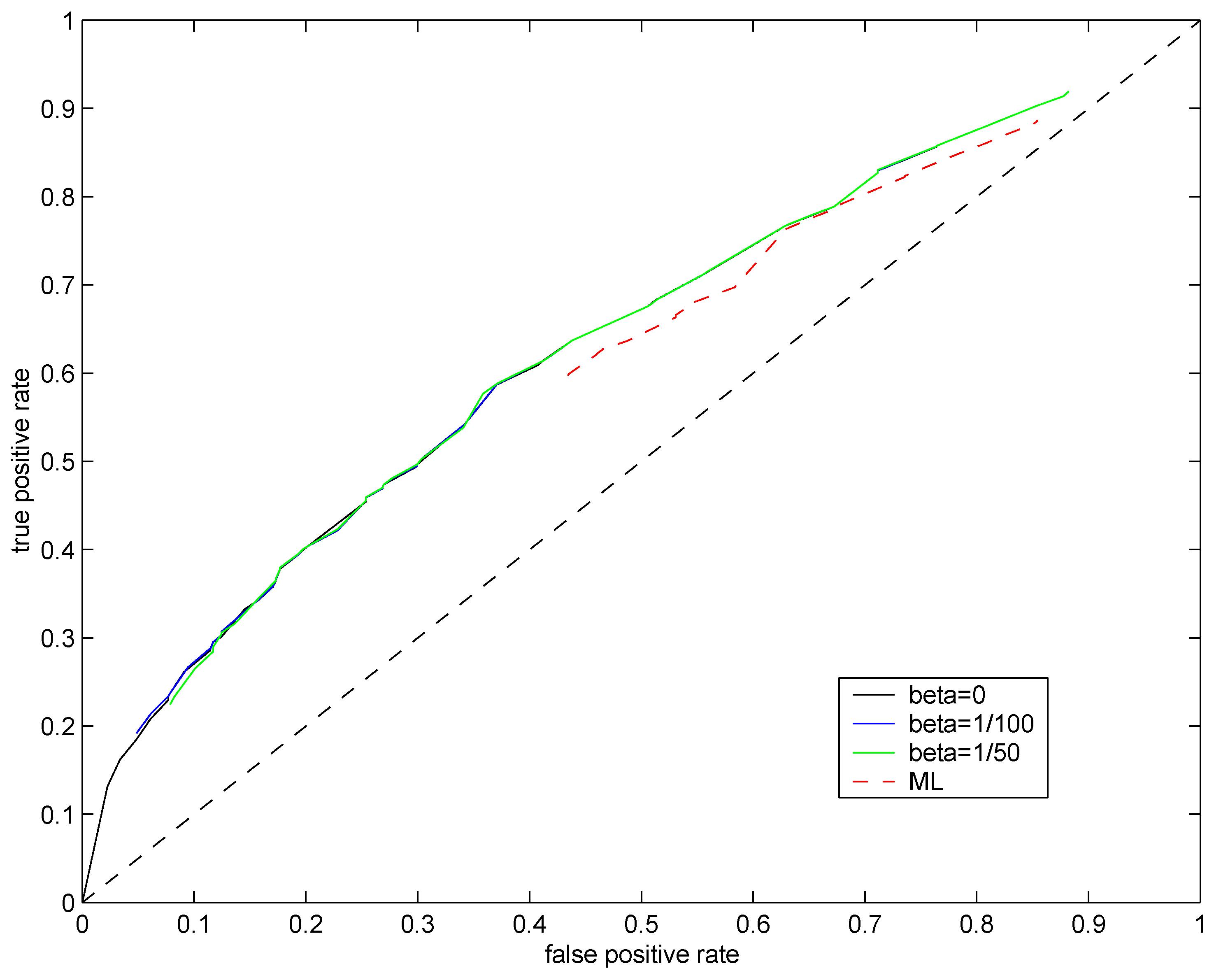
receiver operating characteristic (ROC) curve. If the ROC curve for one test distribution is always above another, this suggests its superiority in classifying genes as differentially expressed. Trivial classification of genes as differentially expressed using a completely random guess would yield the identity (diagonal) ROC curve. ROC curves for the maximum likelihood method (
, red dashed line) and the soft regularization model
,
(solid lines) are plotted in
Figure 5. Not surprisingly, the Bayesian approach (solid lines) outperforms the penalized maximum likelihood one (red dashed line). However, the original
(
, black line) and the soft regularization model (color solid lines) achieve almost identical performances. In this challenging setting (single observations at low mean rate with additional noise), the scheme for setting the regularization parameter
β suggested in
Section 5 has little effect on the resulting classification performance. We also ran experiments to test the “dynamic” scheme for setting
β introduced in
Section 3, but no significant performance improvements were achieved.
Figure 5.
ROC curves for test distributions (solid black line), (solid blue line), (solid green line) and with (dashed red line). Mean rate of the underlying Poisson source was fixed at .
Figure 5.
ROC curves for test distributions (solid black line), (solid blue line), (solid green line) and with (dashed red line). Mean rate of the underlying Poisson source was fixed at .
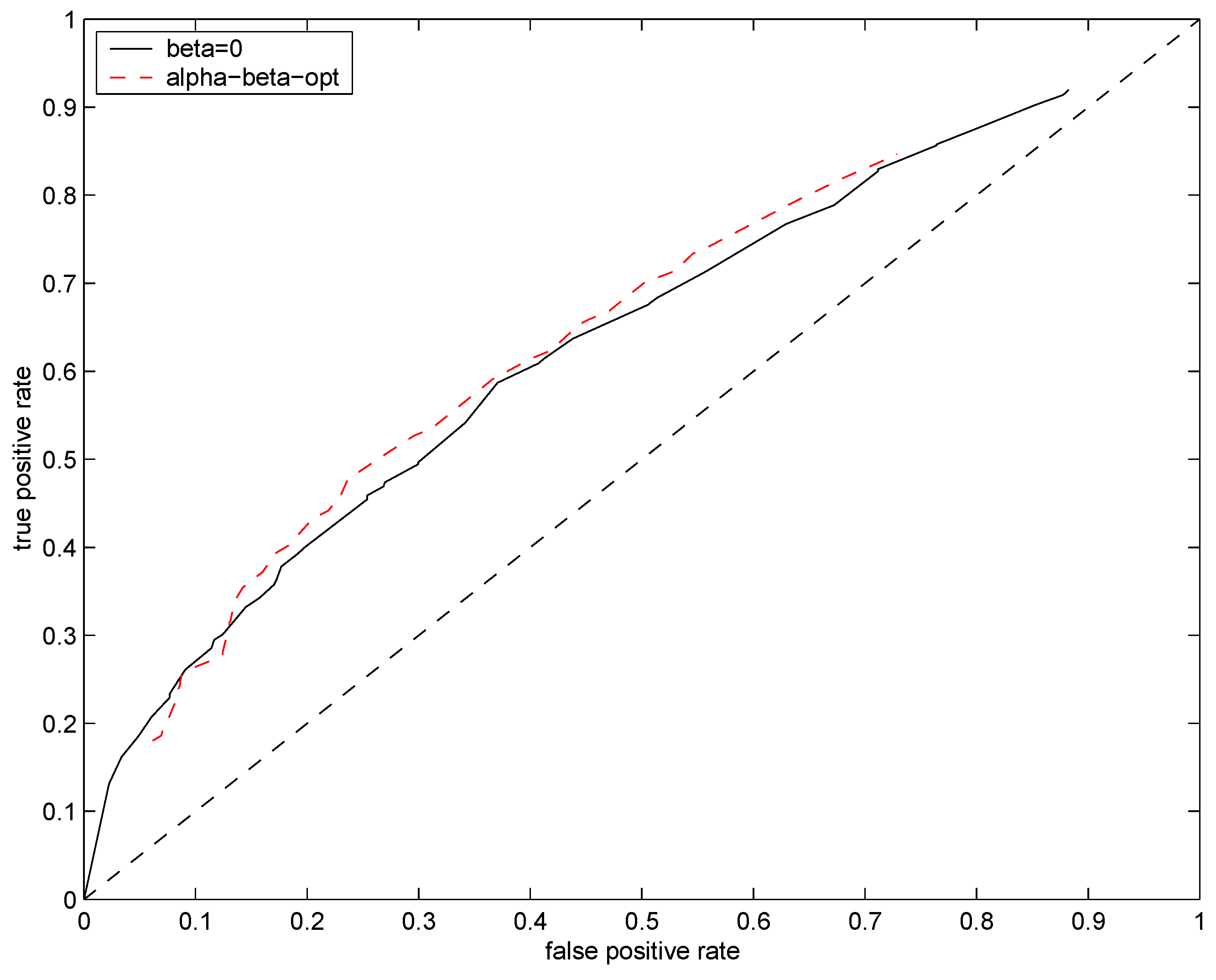
Finally, we devised yet another scheme for determining the hyper-parameters
α and
β of the prior
from the data. In the spirit of type II maximum likelihood, we find the most likely values of
, given the observed counts
, using
where
Using this method, we first optimize the prior hyperparameters on the observed data. The “optimized” prior
now reflects the possible ranges of mean counts
λ one can expect given the data. We then repeated the experiments using the generalized model
derived from the optimized prior. In this way we can assess to what degree the relatively minor performance differences between the generalized and maximum likelihood models in
Figure 5 are due to constraining
α to
(in
), or due to inherent difficulty of learning from single counts. The resulting ROC analysis is shown in
Figure 6. The data driven setting of hyperparameters
leads to slight improvement over
and
.
Figure 6.
ROC curves for test distributions (solid black line) and (dashed red line). Mean rate of the underlying Poisson source was fixed at .
Figure 6.
ROC curves for test distributions (solid black line) and (dashed red line). Mean rate of the underlying Poisson source was fixed at .
