2. Differential Entropy
The entropy of a continuous-valued process is given by its differential entropy. Recall that the entropy of a discrete-valued random variable is given by the Shannon entropy (we shall always choose log base 2 so that entropy will be expressed in units of bits) where pi is the probability of the ith outcome and the sum is over all possible outcomes.
Following [
9] we derive the appropriate expression for differential entropies for conditioned and unconditioned continuous-valued random variables. When a process X is continuous-valued we may approximate it as a discrete-value process by identifying p
i = f
iΔx where f
i is the value of the pdf at the i
th partition point and Δx is the refinement of the partition. We then obtain:
Note that since the X process is continuous-valued, then, as Δx → 0, we have H(X) → + infinity. Thus, for continuous-valued processes, the quantity h(X), when itself defined and finite, is used to represent the entropy of the process. This quantity is known as the differential entropy of random process X.
Closed-form expressions for the differential entropy of many distributions are known. For our purposes, the key expression is the one for the (unconditional) multivariate normal distribution [
10]. Let the probability density function of the n-dimensional random vector x be denoted f(x), then the relevant expressions are:
where detC is the determinant of matrix C, the covariance of x. In what follows, this expression will be used to compute differential entropy of unconditional and conditional normal probability density functions. The case for conditional density functions warrants a little more discussion.
Recall that the relationships between the joint and conditional covariance matrices, C
XY and C
Y|X, respectively, of two random variables X and Y (having dimensions n
x and n
y, respectively) are given by:
Here blocks Σ11 and Σ22 have dimensions nx by nx and ny by ny, respectively. Now, using Leibniz’s formula, we have that:
Hence the conditional differential entropy of Y, given X, may be conveniently computed using:
This formulation is very handy as it allows us to compute many information-theoretic quantities with ease. The strategy is as follows. We define C
(k) to be the covariance of two random processes sampled at k consecutive timestamps {t
n−k+2, t
n− k+1, …, t
n, t
n+1}. We then compute transfer entropies for values of k up to k sufficiently large to ensure that their valuations do not change significantly if k is further increased. For our examples, we have found k = 10 to be more than sufficient. A discussion of the importance of considering this sufficiency is provided in [
11].
3. Transfer Entropy Computation Using Variable Number of Timestamps
We wish to consider two example processes each of which conforms to one of the two model systems having the general expressions:
and:
Here, vn and wn are zero mean uncorrelated Gaussian noise processes having variances R and Q, respectively. For system stability, we require the model poles to lie within the unit circle.The first model is of a filtered process noise X one-way coupled to an instantaneous, but noisy measurement process Y. The second model is a two-way coupled pair of processes, X and Y.
Transfer entropy (as defined by Schreiber [
1]) considers the flow of information from past states (
i.e., state values having, timetags
) of one process to the present
state of another process. However, note that in the first general model (measurement process) there is an explicit flow of information from the present state of the X process; x
n+1 determines the present state of the Y process y
n+1 (assuming c
− 1 is not zero). To fully capture the information transfer from the X process to the current state of the Y process we must identify the correct causal states [
4]. For the measurement system, the causal states include the current (present) state. This state is not included in the definition of transfer entropy, being a mutual information quantity conditioned on only past states. Hence, for the purpose of this paper, we will temporarily define a quantity, “information transfer,” similar to transfer entropy, except that the present of the driving process, x
n+1, will be lumped in with the past values of the X process: x
n−k+2:x
n. For the first general model there is no information transferred from the Y to the X process. We define the (non-zero) information transfer from the X to the Y process (based on data from k timetags) as:
The major contribution of this paper is to show how to analytically compute transfer entropy for AR Gaussian processes using an iterative method for computing the required covariance matrices. Computation of information transfer is additionally presented to elucidate the power of the method when similar information quantities are of interest and to make the measurement example more interesting. We now present a general method for computing the covariance matrices required to compute information-theoretic quantities for the AR models above. Two numerical examples follow.
To compute transfer entropy over a variable number of multiple time lags for AR processes of the general types shown above, we compute its block entropy components over multiple time lags. By virtue of the fact that the processes are Gaussian we can avail ourselves of analytical entropy expressions that depend only on the covariance of the processes. In this section we show how to analytically obtain the required covariance expressions starting with the covariance for a single time instance. Taking expectations, using the AR equations, we obtain the necessary statistics to characterize the process. Representing these expectation results in general, the process covariance matrix C
(1)(t
n) corresponding to a single timestamp, t
n, is:
To obtain an expanded covariance matrix, accounting for two time instances (t
n and t
n+1), we compute the additional expectations required to fill in the matrix C
(2)(t
n):
Because the process is stationary, we may write:
where:
Thus we have found the covariance matrix C(2) required to compute block entropies based on two timetags or, equivalently, one time lag. Using this matrix the single-lag transfer entropies may be computed.
We now show how to compute the covariance matrices corresponding to any finite number of time stamps. Define vector
. Using the definitions above, write the matrix C
(2) as a block matrix and, using standard formulas, compute the conditional mean and covariance C
c of
given
:
Note that the expected value of the conditional mean is zero since the mean of the process, , is itself zero.
With these expressions in hand, we note that we may view propagation of the state
to its value
at the next timestamp as accomplished by the recursion:
Here S is the principal square root of the matrix C
c. It is conveniently computed using the inbuilt Matlab function
sqrtm. To see analytically that the recursion works, note that using it we recover at each timestamp a process having the correct mean and covariance:
and:
Thus, because the process is Gaussian and fully specified by its mean and covariance, we have verified that the recursive representation yields consistent statistics for the stationary AR system. Using the above insights, we may now recursively compute the covariance matrix C(k) for a variable number (k) of timestamps. Note that C(k) has dimensions of 2k × 2k. We denote 2 × 2 blocks of C(k) as C(k)ij for i, j = 1,2, ..., k , where C(k)ij is the 2-by-2 block of C(k) consisting of the four elements of C(k) that are individually located in row 2i − 1 or 2i and column 2j − 1 or 2j.
The above recursion is now used to compute the block elements of C
(3). Then each of these block elements is, in turn, expressed in terms of block elements of C
(2). These calculations are shown in detail below where we have also used the fact that the mean of the z
n vector is zero:
By continuation of this calculation to larger timestamp blocks (k > 3), we find the following pattern that can be used to extend (augment) C
(k−1) to yield C
(k). The pattern consists of setting most of the augmented matrix equal to that of the previous one, and then computing two additional rows and columns for C
(k), k > 2, to fill out the remaining elements. The general expressions are:
At this point in the development we have shown how to compute the covariance matrix:
Since the system is linear and the process noise w
n and measurement noise v
n are white zero-mean Gaussian noise processes, we may express the joint probability density function for the 2k variates as:
Note that the mean of all 2k variates is zero.
Finally, to obtain empirical confirmation of the equivalence of the covariance terms obtained using the original AR system and its recursive representation, numerical simulations were conducted. Using the example 1 system (below) 500 sequences were generated each of length one million. For each sequence the C(3) covariance was computed. The error for all C(3) matrices was then averaged, assuming that the C(3) matrix calculated using the method based on the recursive representation was the true value. The result was that for each of the matrix elements, the error was less than 0.0071% of its true value. We are now in position to compute transfer entropies for a couple of illustrative examples.
4. Example 1: A One-Way Coupled System
For this example we consider the following system:
Parameter hc specifies the coupling strength of the Y process to the first-order AR process X, and R and Q are their respective (wn and vn) zero-mean Gaussian process noise variances. For stability, we require |a| <1. Comparing to the first general representation given above, we have m = 0, and . The system models filtered noise xn and a noisy measurement, yn, of xn. Thus the xn sequence represents a hidden process (or model) which is observable by way of another sequence, yn. We wish to examine the behavior of transfer entropy as a function of the correlation ρ between xn and yn. One might expect that the correlation ρ between xn and yn to be proportional of the degree of information flow; however, we will see that the relationship between transfer entropy and correlation is not quite that simple.
Both the X and Y processes have zero mean. Computing the joint covariance matrix C
(1) for x
n and y
n and their correlation we obtain:
Hence the process covariance matrix C
(1) corresponding to a single timestamp, t
n is:
In order to obtain an expanded covariance matrix, accounting for two time instances (t
n and t
n+1) we compute the additional expectations required to fill in the matrix C
(2):
Thus we have found the covariance matrix C(2) required to compute block entropies based on a single time lag. Using this matrix the single-lag transfer entropies may be computed. Using the recursive process described in the previous section we can compute C(1°). We have found that using higher lags does not change the entropy values significantly.
To aid the reader in understanding the calculations required to compute transfer entropies using higher time lags, it is worthwhile to compute transfer entropy for a single lag. We first define transfer entropy using general notation indicating the partitioning of the X and Y sequences in to past and future
and
, respectively. We then compute transfer entropy as a sum of block entropies:
The Y states have no influence on the X sequence in this example. Hence TE
y→x = 0. Since we are here computing transfer entropy for a single lag (
i.e., two time tags t
n and t
n+1) we have:
By substitution of the expression for the differential entropy of each block we obtain:
For this example, note from the equation for y
n+1 that state x
n+1 is a causal state of X influencing the value of y
n+1. In fact, it is the most important such state. To capture the full information that is transferred from the X process to the Y process over the course of two time tags we need to include state x
n+1. Hence we compute the information transfer from x → y as:
Here the notation
indicates the determinant of the matrix composed of the rows and columns of C
(2) indicated by the list of indices i shown in the subscripted brackets. For example,
is the determinant of the matrix formed by extracting columns {1, 2, 3, 4} and rows {1, 2, 3, 4} from matrix C
(2). In later calculations we will use slightly more complicated-looking notation. For example,
is the determinant of the matrix formed by extracting columns {2, 4 ,…, 18, 20} and the same-numbered rows from matrix C
(1°
). (Note C
(k)[i],[i] is not the same as C
(k)ii as used in
Section 3).
It is interesting to note that a simplification in the expression for information transfer can be obtained by writing the expression for it in terms of conditional entropies:
From the fact that y
n+1 = x
n+1 + v
n+1 we see immediately that:
To compute transfer entropy using nine lags (ten timestamps) assume that we have already computed C
(10) as defined above. We partition the sequence
into three subsets:
Now, using these definitions, and substituting in expressions for differential block entropies we obtain:
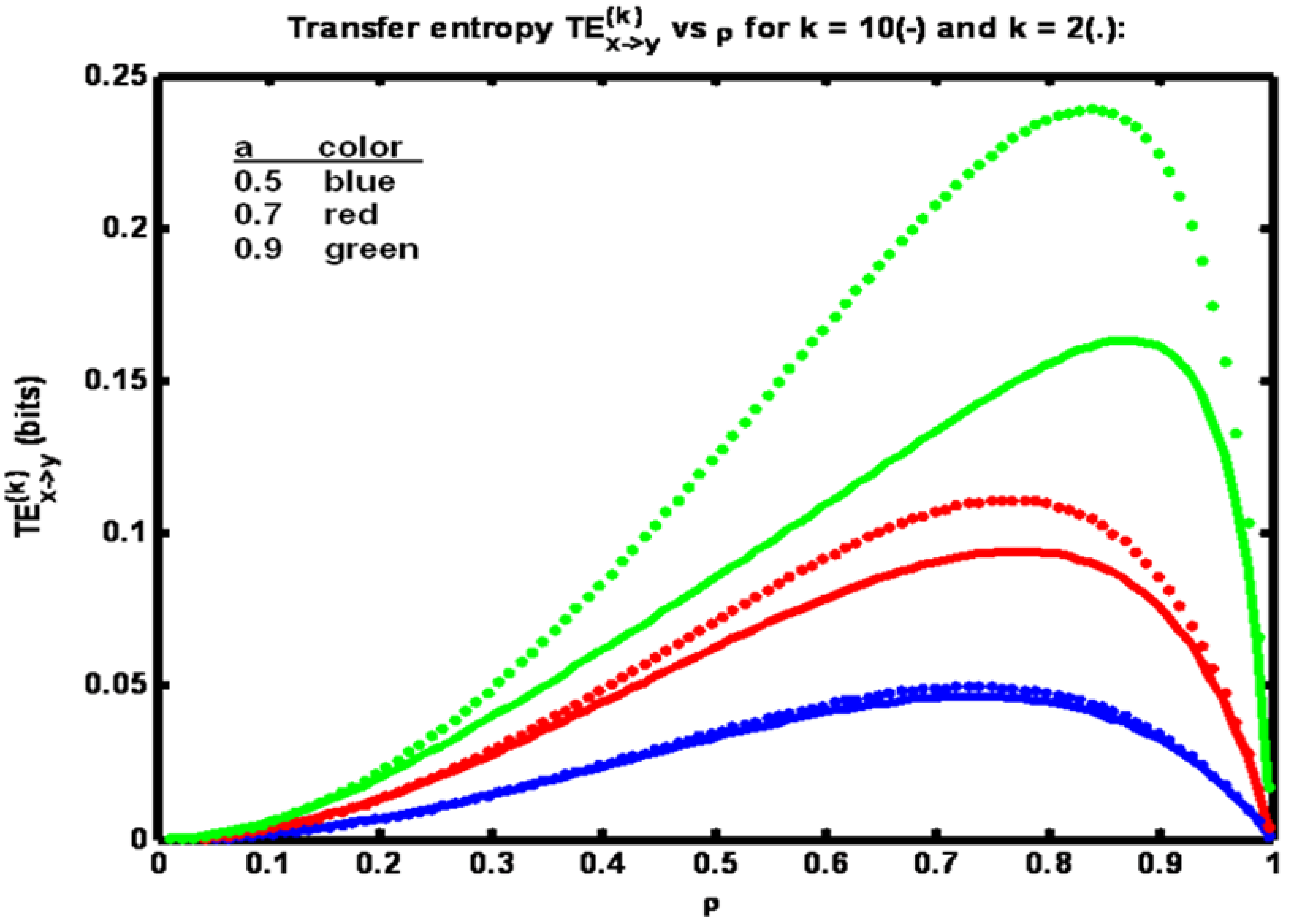
As a numerical example we set hc = 1, Q = 1, and for three different values of a (0.5, 0.7 and 0.9) we vary R so as to scan the correlation ρ between the x and y processes between the values of 0 and 1.
In
Figure 1 it is seen that for each value of parameter
a there is a peak in the transfer entropy TE
(k)x→y. As the correlation ρ between x
n and y
n increases from a low value the transfer entropy increases since the amount of information shared between y
n+1 and x
n is increasing. At a critical value of ρ transfer entropy peaks and then starts to decrease. This decrease is due to the fact that at high values of ρ the measurement noise variance R is small. Hence y
n becomes very close to equaling x
n so that the amount of information gained (about y
n+1) by learning x
n, given y
n, becomes small. Hence h(y
n+1 | y
n) ‑ h(y
n+1 | y
n, x
n) is small. This difference is TE
(2)x→y.
Figure 1.
Example 1: Transfer entropy TE(k)x→y versus correlation coefficient ρ for three values of parameter a (see legend). Solid trace: k = 10, dotted trace: k = 2.
Figure 1.
Example 1: Transfer entropy TE(k)x→y versus correlation coefficient ρ for three values of parameter a (see legend). Solid trace: k = 10, dotted trace: k = 2.
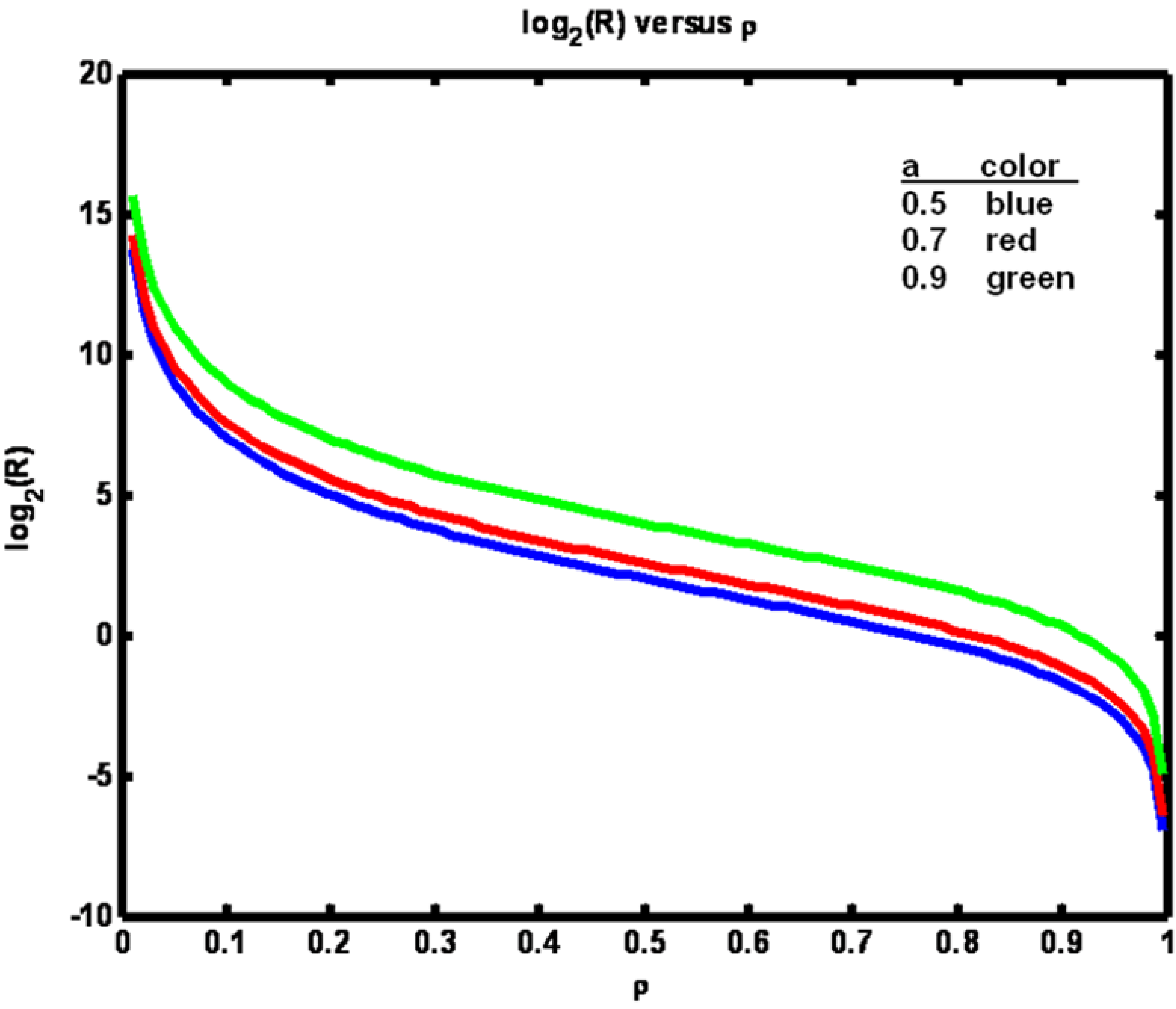
The relationship between ρ and R is shown in
Figure 2. Note that when parameter
a is increased, a larger value of R is required to maintain ρ at a fixed value. Also, in
Figure 1 we see the effect of including more timetags in the analysis. When k is increased from 2 to 10 transfer entropy values fall, particularly for the largest value of parameter
a. It is known that entropies decline when conditioned on additional variables. Here, transfer entropy is acting similarly. In general, however, transfer entropy, being a mutual information quantity, has the property that conditioning could make it increase as well [
12].
Figure 2.
Example 1: Logarithm of R versus ρ for three values of parameter a (see legend).
Figure 2.
Example 1: Logarithm of R versus ρ for three values of parameter a (see legend).
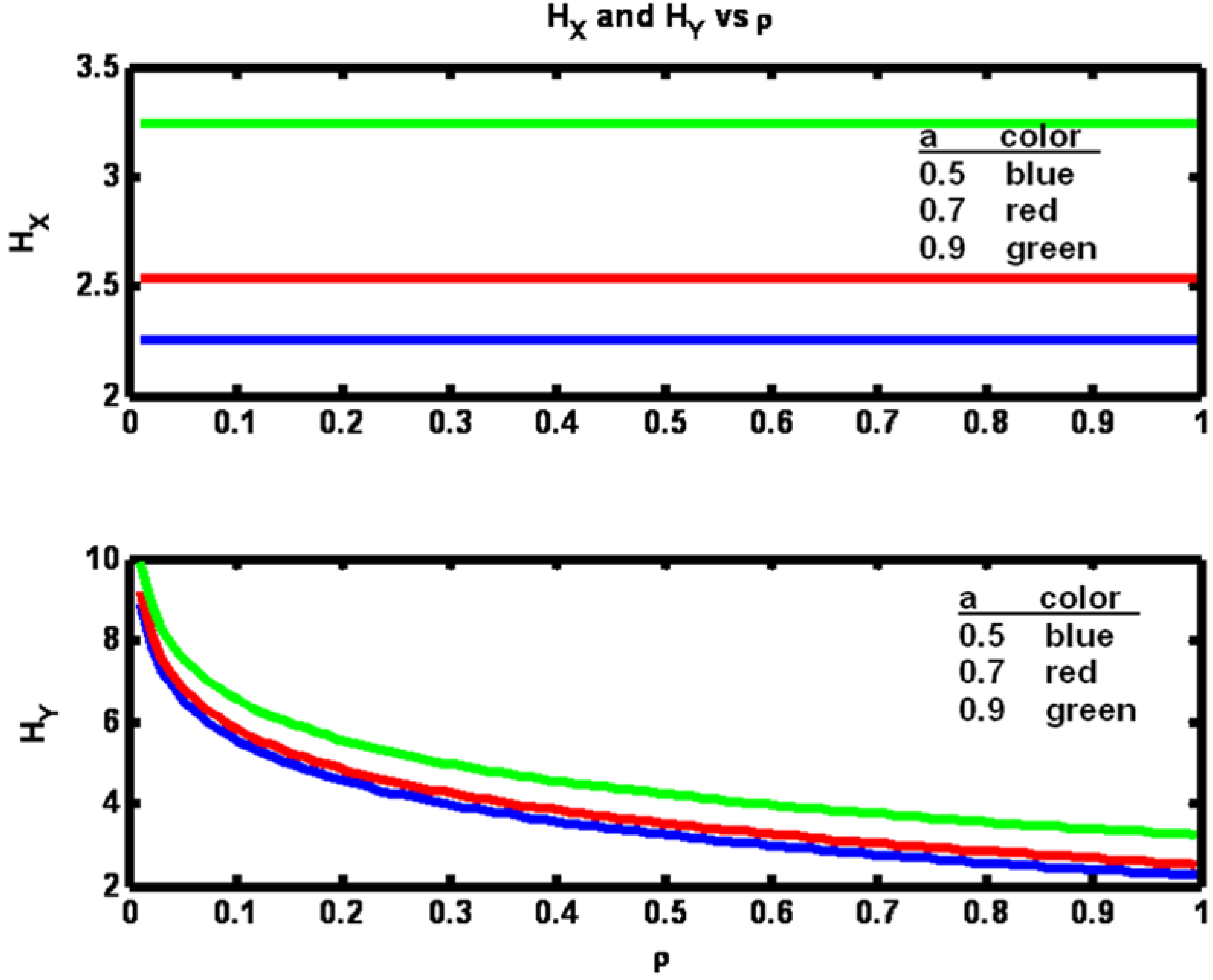
The observation that the transfer entropy decrease is greatest for the largest value of parameter
a is perhaps due to the fact that the entropy of the X process is itself greatest for the largest
a value and therefore has more sensitivity to an increase in X data availability (
Figure 3).
From
Figure 1 it is seen that as the value of parameter
a is increased, transfer entropy is increased for a fixed value of ρ. The reason for this increase may be gleaned from
Figure 3 where it is clear that the amount of information contained in the x process, H
X, is greater for larger values of
a. Hence more information is available to be transferred at the fixed value of ρ when
a is larger. In the lower half of
Figure 3 we see that as ρ increases the entropy of the Y process, H
Y, approaches the value of H
X. This result is due to the fact that the mechanism being used to increase ρ is to decrease R. Hence as R drops close to zero y
n looks increasingly identical to x
n (since h
c = 1).
Figure 3.
Example 1: Process entropies HX and HY versus correlation coefficient ρ for three values of parameter a (see legend).
Figure 3.
Example 1: Process entropies HX and HY versus correlation coefficient ρ for three values of parameter a (see legend).
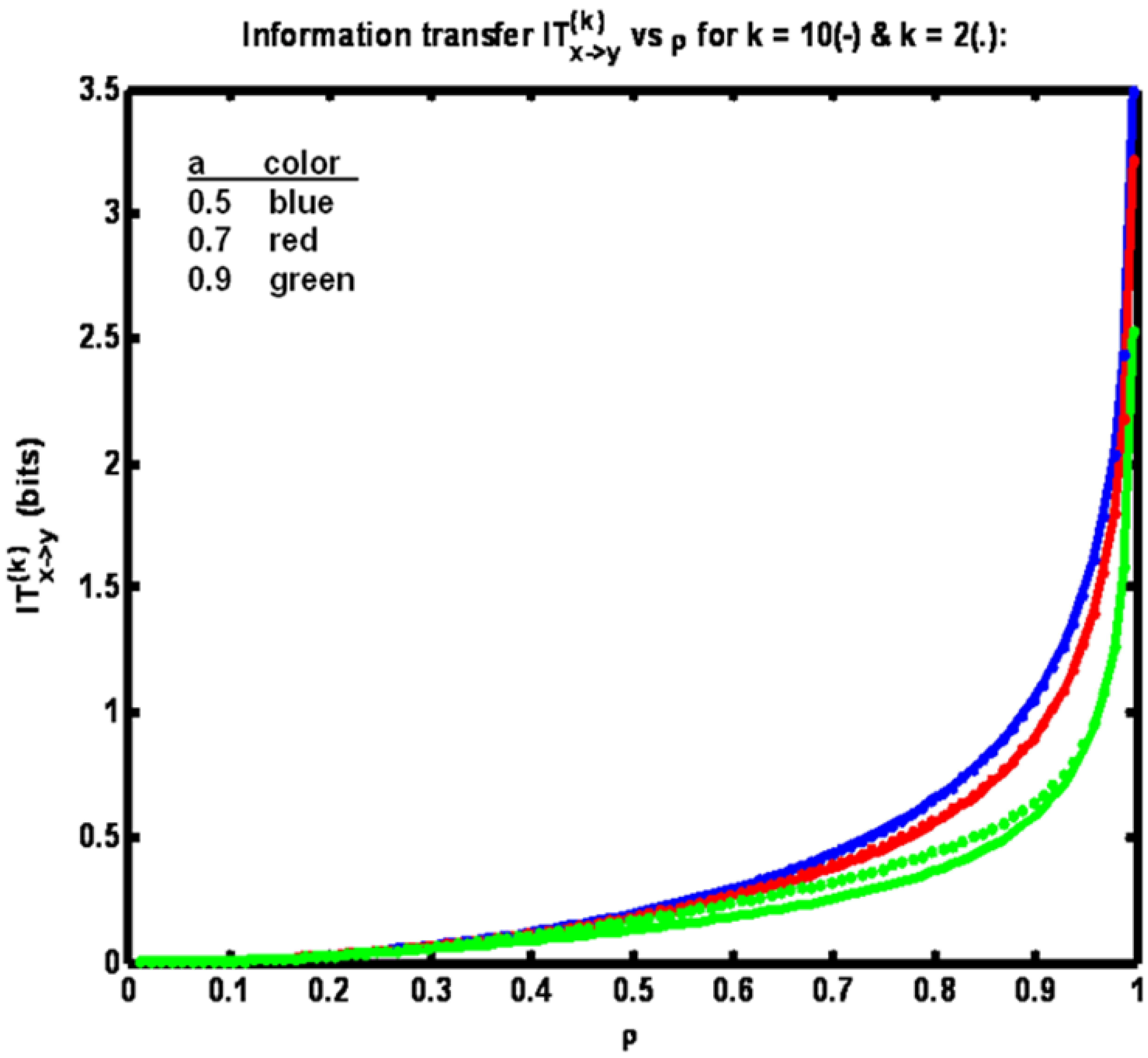
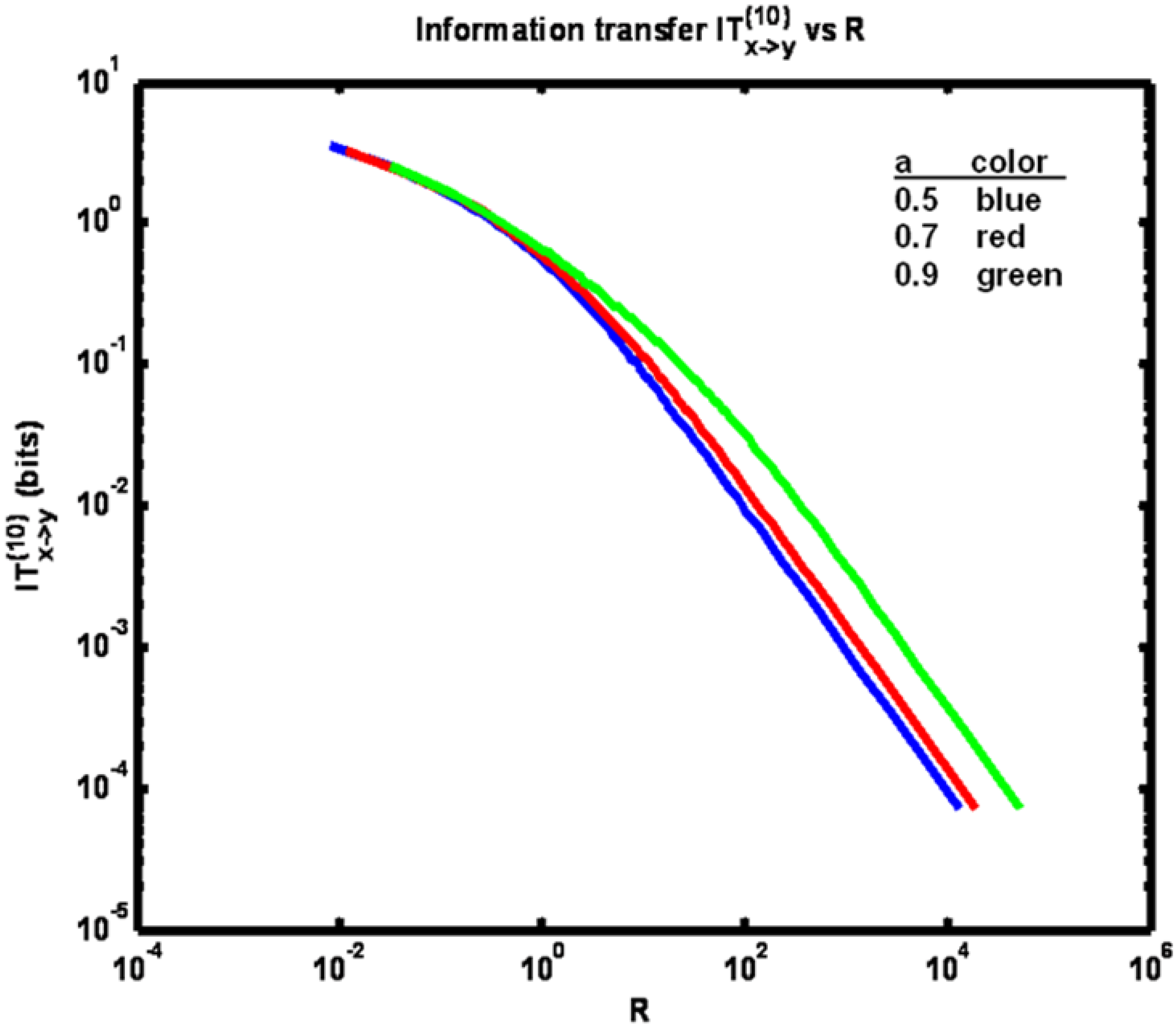
Figure 4 shows information transfer IT
(k)x→y plotted
versus correlation coefficient ρ. Now note that the trend is for information transfer to increase as ρ is increased over its full range of values. °
Figure 4.
Example 1: Information transfer IT(k)x→y versus correlation coefficient ρ for three different values of parameter a (see legend) for k = 10 (solid trace) and k = 2 (dotted trace).
Figure 4.
Example 1: Information transfer IT(k)x→y versus correlation coefficient ρ for three different values of parameter a (see legend) for k = 10 (solid trace) and k = 2 (dotted trace).
This result is obtained since as ρ is increased y
n+1 becomes increasingly correlated with x
n+1. Also, for a fixed ρ, the lowest information transfer occurs for the largest value of parameter
a. We obtain this result since at the higher
a values x
n and x
n+1 are more correlated. Thus the benefit of learning the value of y
n+1 through knowledge of x
n+1 is relatively reduced, given that y
n (itself correlated with x
n) is presumed known. Finally, we have IT
(10)x→y < IT
(2)x→y since conditioning the entropy quantities comprising the expression for information transfer with more state data acts to reduce their difference. Also, by comparison of
Figure 2 and
Figure 4, it is seen that information transfer is much greater than transfer entropy. This relationship is expected since information transfer as defined herein (for k = 2) is the amount of information that is gained about y
n+1 from learning x
n+1 and x
n, given that y
n is already known. Whereas transfer entropy (for k = 2) is the information gained about y
n+1 from learning only x
n, given that y
n is known. Since the state y
n+1 in fact equals x
n+1, plus noise, learning x
n+1 is highly informative, especially when the noise variance is small (corresponding to high values of ρ). The difference between transfer entropy and information transfer therefore quantifies the benefit of learning x
n+1, given that x
n and y
n are known (when the goal is to determine y
n+1).
Figure 5 shows how information transfer varies with measurement noise variance R. As R increases the information transfer decreases since measurement noise makes determination of the value of y
n+1 from knowledge of x
n and x
n+1 less accurate. Now, for a fixed R, the greatest value for information transfer occurs for the greatest value of parameter
a. This is the opposite of what we obtained for a fixed value of ρ as shown in
Figure 4. The way to see the rationale for this is to note that, for a fixed value of information transfer, R is highest for the largest value of parameter
a. This result is obtained since larger values of
a yield the most correlation between states x
n and x
n+1. Hence, even though the measurement y
n+1 of x
n+1 is more corrupted by noise (due to higher R), the same information transfer is achieved nevertheless, because x
n provides a good estimate of x
n+1 and, thus, of y
n+1.
Figure 5.
Example 1: Information transfer IT(10)x→y versus measurement error variance R for three different values of parameter a (see legend).
Figure 5.
Example 1: Information transfer IT(10)x→y versus measurement error variance R for three different values of parameter a (see legend).
5. Example 2: Information-theoretic Analysis of Two Coupled AR Processes.
In example 1 the information flow was unidirectional. We now consider a bidirectional example achieved by coupling two AR processes. One question we may ask in such a system is how transfer entropies change with variations in correlation and coupling coefficient parameters. It might be anticipated that increasing either of these quantities will have the effect of increasing information flow and thus transfer entropies will increase.
The system is defined by the equations:
For stability, we require that the eigenvalues of the constant matrix
lie in the unit circle. The means of processes X and Y are zero. The terms w
n and v
n are the X and Y processes noise terms respectively. Using the following definitions:
we may solve for the correlation coefficient ρ between x
n and y
n to obtain:
Now, as we did previously in example 1 above, compute the covariance C
(2) of the variates obtained at two consecutive timestamps to yield:
At this point the difficult part is done and the same calculations can be made as in example 1 to obtain C
(k); k = 3,4, …, 10 and transfer entropies. For illustration purposes, we define the parameters of the system as shown below, yielding a symmetrically coupled pair of processes. To generate a family of curves for each transfer entropy we choose a fixed coupling term ε from a set of four values. We set Q = 1000 and vary R so that ρ varies from about 0 to 1. For each ρ value we compute the transfer entropies. The relevant system equations and parameters are:
Hence, we make the following substitutions to compute C
(2):
For each parameter set {ε, Q, R} there is a maximum possible ρ,
obtained by taking the limit as R→ ∞ of the expression for ρ given above. Doing so, we obtain:
where:
There is a minimum value of ρ also. The corresponding value for R, R
min, was found by means of the inbuilt Matlab program
fminbnd. This program is designed to find the minimum of a function in this case ρ(
a,
b,
c,
d, R, Q)) with respect to one parameter (in this case R) starting from an initial guess (here, R = 500). The program returns the minimum functional value (ρ
min) and the value of the parameter at which the minimum is achieved (R
min). After identifying R
min a set of R values were computed so that the corresponding set of ρ values spanned from ρ
min to the maximum
in fixed increments of Δρ (here equal to 0.002). This set of R values was generated using the iteration:
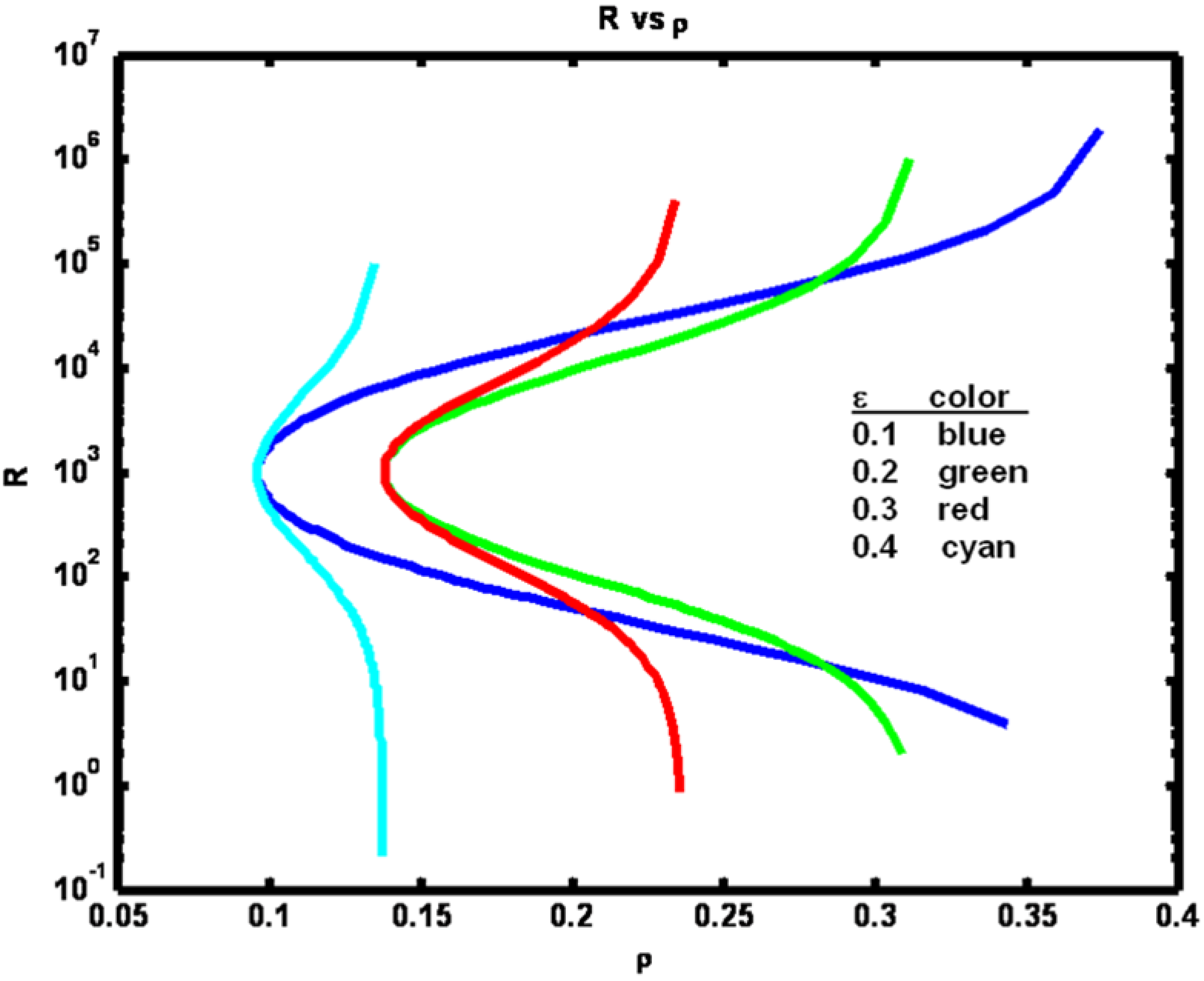
For the four selections of parameter ε we obtain the functional relationships shown in
Figure 6.
From
Figure 6 we see that for a fixed ε, increasing R increases (or decreases) ρ depending on whether R is less than (or greater than) Q (Q = 1000). Note that large increases in R > Q are required to marginally increase ρ when ρ nears its maximum value. The reason that the minimum ρ value occurs when Q equals R is because whenever they are unequal one of the processes dominates the other, leading to increased correlation. Also, note that if R << Q, then increasing ε will cause ρ to decrease since increasing the coupling will cause the variance of the y process Var(y
n), a term appearing in the denominator of the expression for ρ, to increase. If Q << R, a similar result is obtained when ε is increased.
Figure 6.
Example 2: Process noise variance R versus correlation coefficient ρ for a set of ε parameter values (see figure legend).
Figure 6.
Example 2: Process noise variance R versus correlation coefficient ρ for a set of ε parameter values (see figure legend).
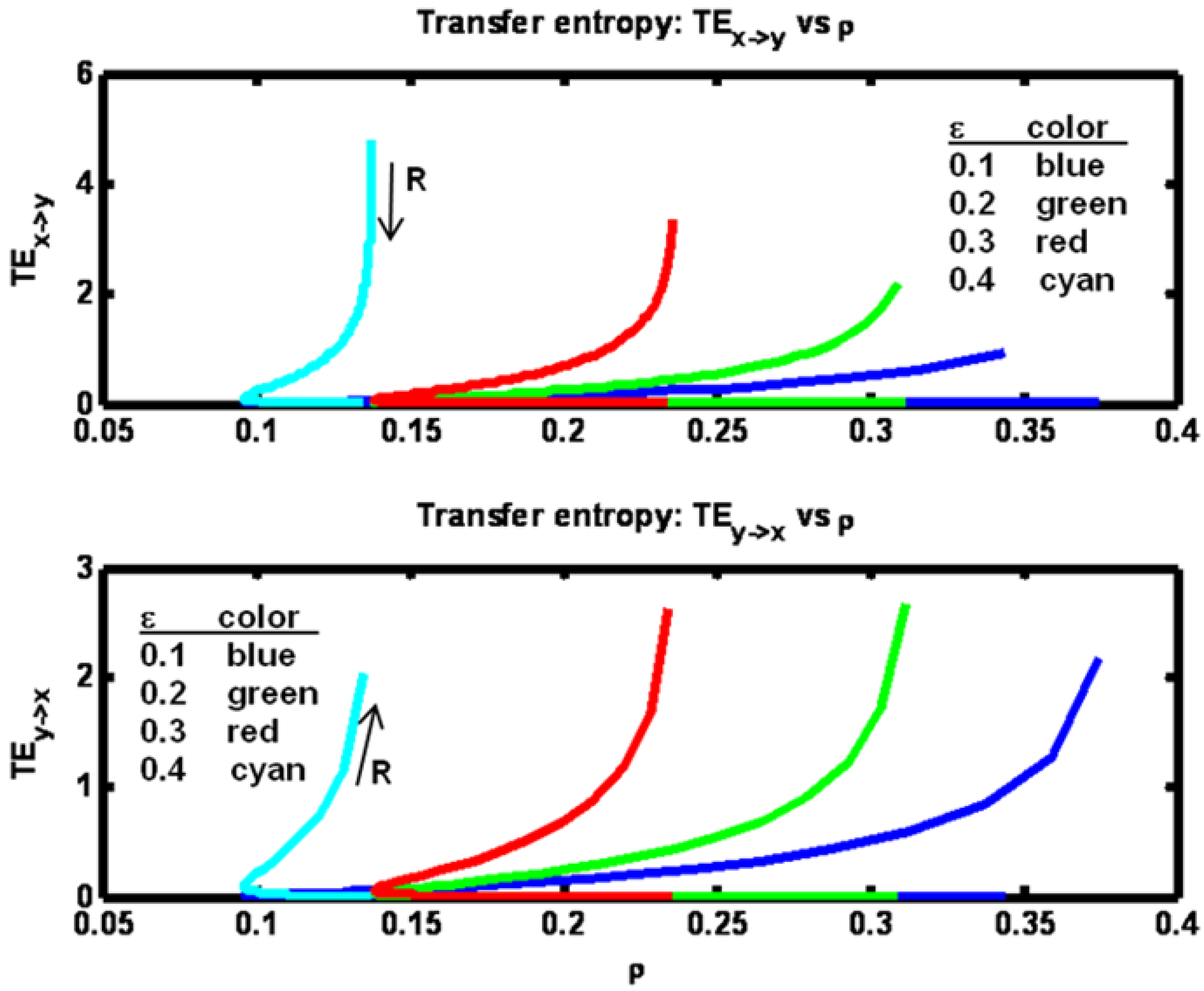
Transfer entropies in both directions are shown in
Figure 7. Fixing ε, we note that as R is increased from a low value both ρ and TE
x− >y initially decrease while TE
y− >x increases. Then for further increases of R, ρ reaches a minimum value then begins to increase, while TE
x→y continues to decrease and TE
y→x continues to increase.
Figure 7.
Example 2: Transfer entropy values versus correlation ρ for a set of ε parameter values (see figure legend). Arrows indicate direction of increasing R values.
Figure 7.
Example 2: Transfer entropy values versus correlation ρ for a set of ε parameter values (see figure legend). Arrows indicate direction of increasing R values.
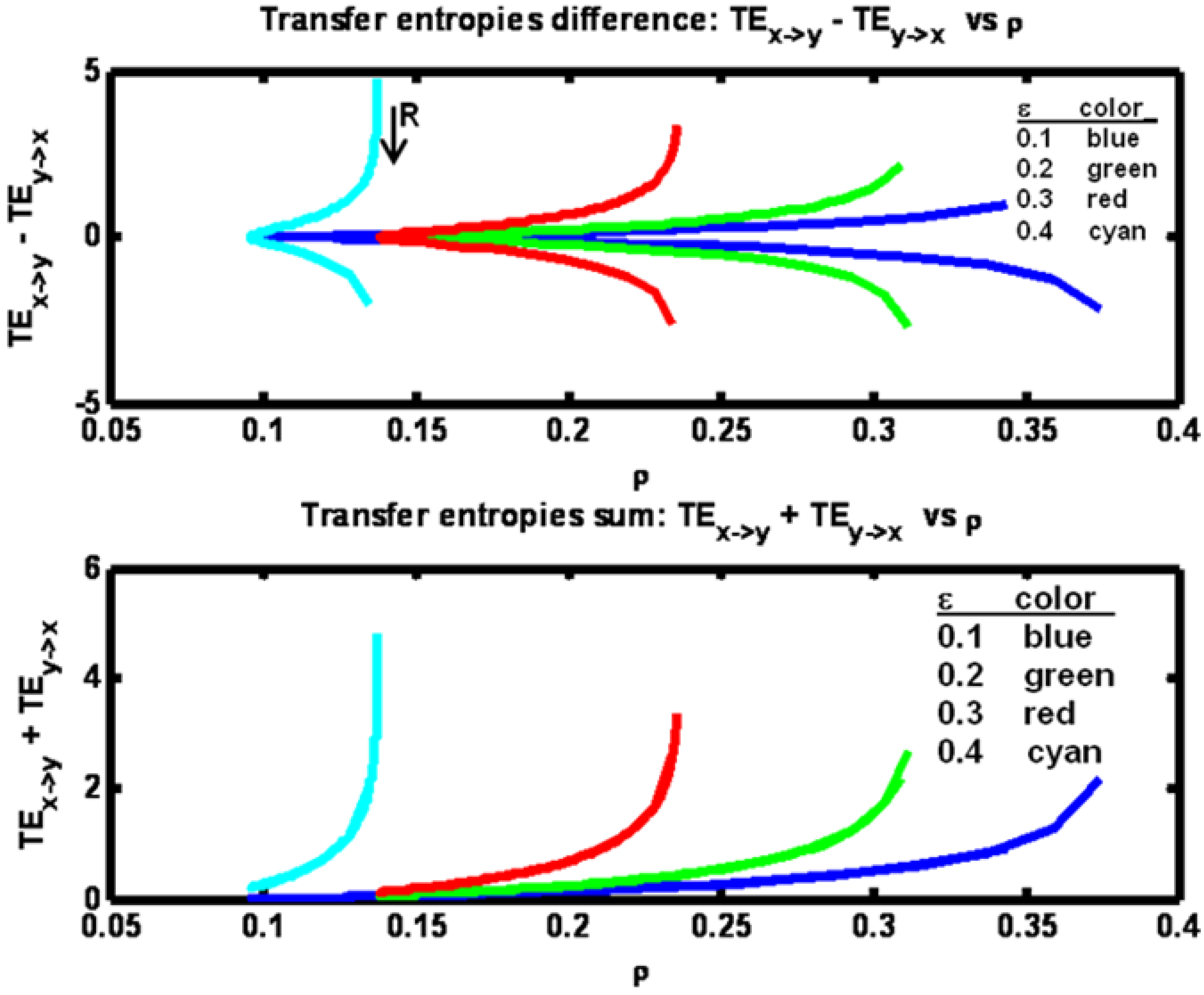
Figure 8.
Example 2: Transfer entropies difference (TEx− >y – TEy − > x) and sum (TEx− > y + TEy− > x) versus correlation ρ for a set of ε parameter values (see figure legend). Arrow indicates direction of increasing R values.
Figure 8.
Example 2: Transfer entropies difference (TEx− >y – TEy − > x) and sum (TEx− > y + TEy− > x) versus correlation ρ for a set of ε parameter values (see figure legend). Arrow indicates direction of increasing R values.
By plotting the difference TE
x→y – TE
y→x in
Figure 8 we see the symmetry that arises as R increases from a low value to a high value. What is happening is that when R is low, the X process dominates the Y process so that TE
x→y > TE
y→x. As R increases, the two entropies equilibrate. Then, as R rises above Q, the Y process dominates giving TE
x→y < TE
y→x. The sum of the transfer entropies shown in
Figure 8 reveal that the total information transfer is minimal at the minimum value of ρ and increases monotonically with ρ. The minimum value for ρ in this example occurs when the process noise variances Q and R are equal (matched).
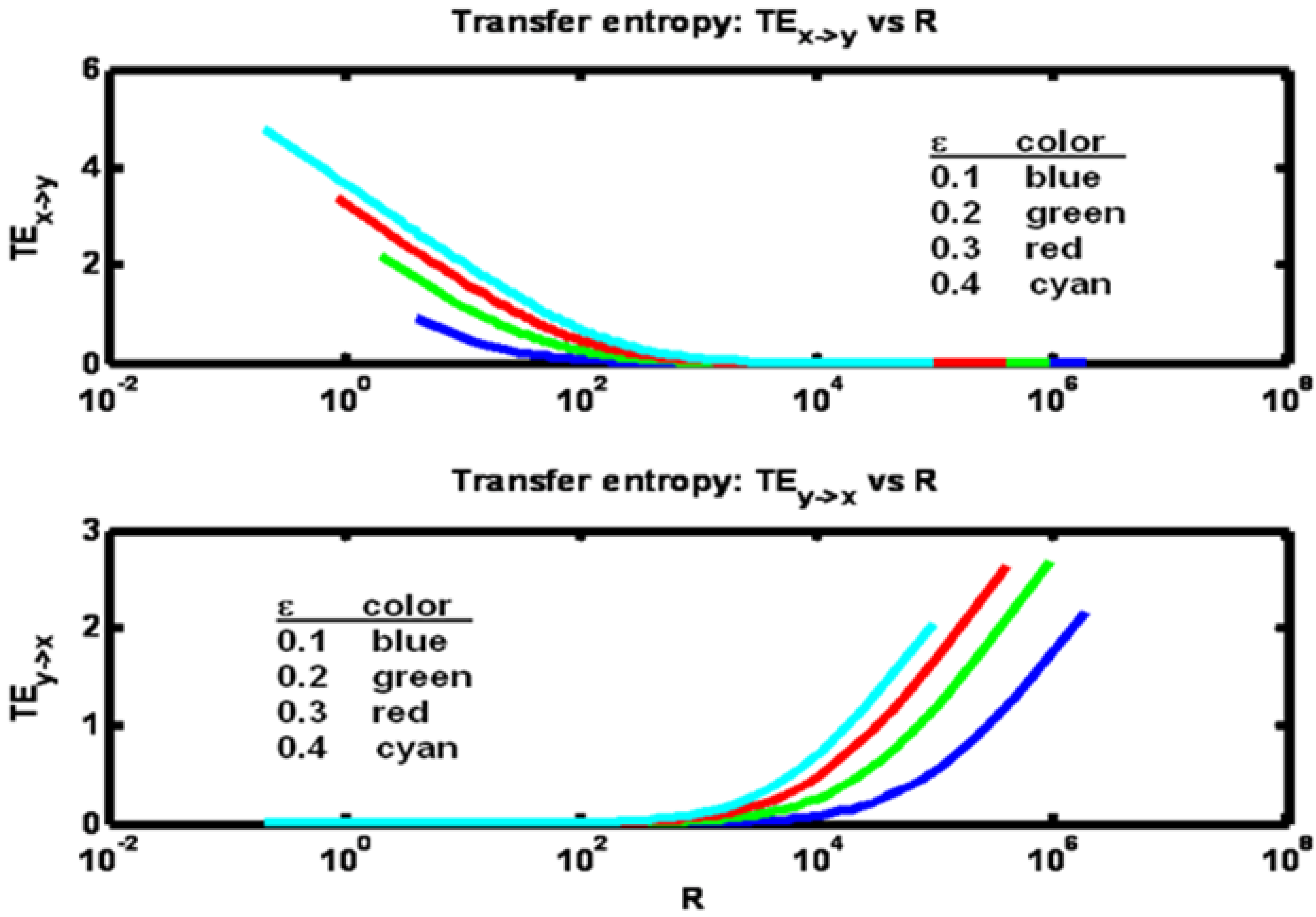
Figure 9 shows the changes in the transfer entropy values explicitly as a function of R. Clearly, when R is small (as compared to Q = 1000), TE
x→y > TE
y→x. Also it is clear that at every fixed value of R, both transfer entropies are higher at the larger values for the coupling term ε.
Figure 9.
Example 2: Transfer entropies TEx→y and TEy→x versus process noise variance R for a set of ε parameter values (see figure legend).
Figure 9.
Example 2: Transfer entropies TEx→y and TEy→x versus process noise variance R for a set of ε parameter values (see figure legend).
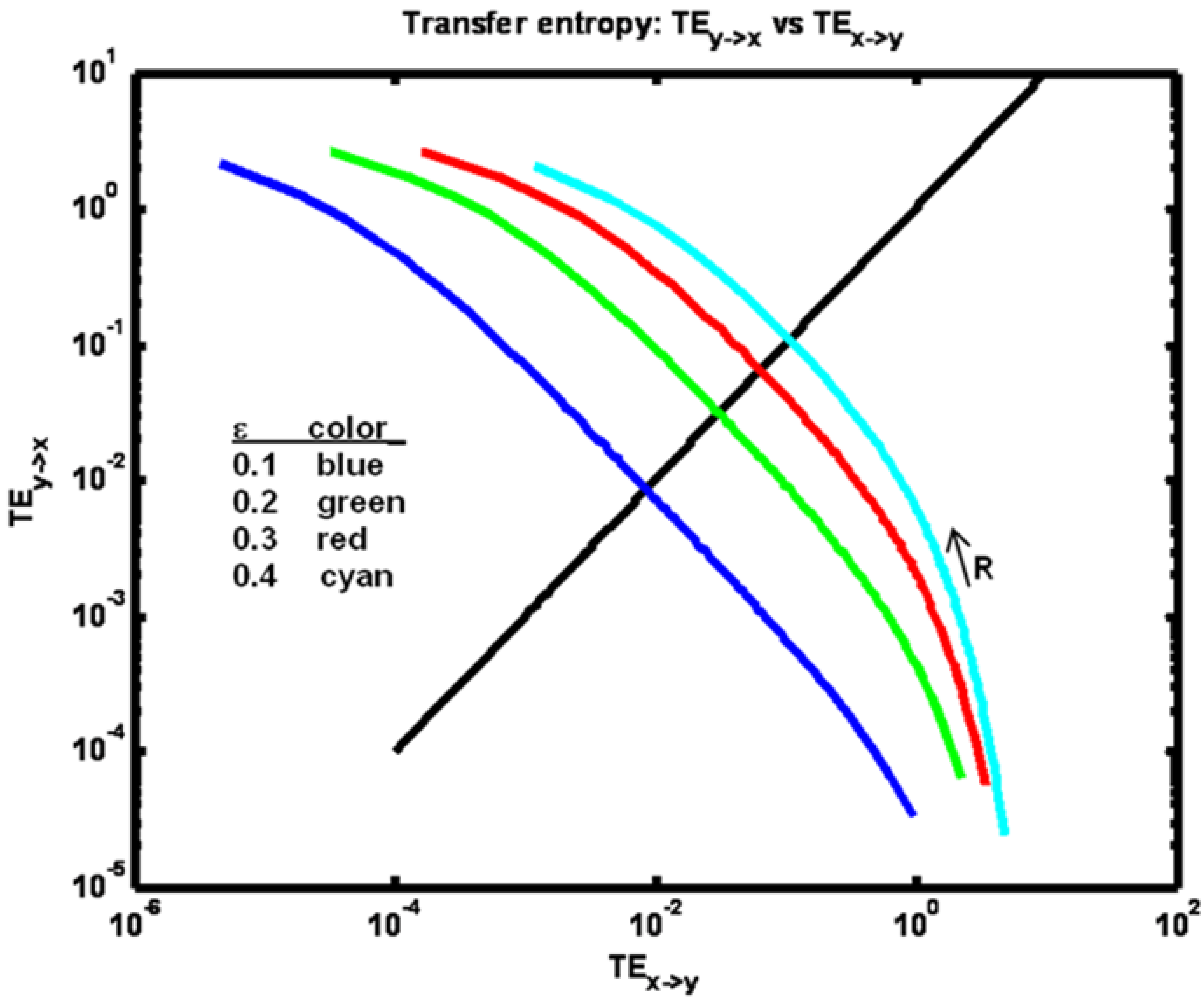
Another informative view is obtained by plotting one transfer entropy value
versus the other as shown in
Figure 10.
Figure 10.
Example 2: Transfer entropy TEx− > y plotted versus TEy− > x for a set of ε parameter values (see figure legend). The black diagonal line indicates locations where equality obtains. Arrow indicates direction of increasing R values.
Figure 10.
Example 2: Transfer entropy TEx− > y plotted versus TEy− > x for a set of ε parameter values (see figure legend). The black diagonal line indicates locations where equality obtains. Arrow indicates direction of increasing R values.
Here it is evident how TEy→x increases from a value less than TEx→y to a value greater than TEx→y as R increases. Note that for higher coupling values ε this relative increase is more abrupt.
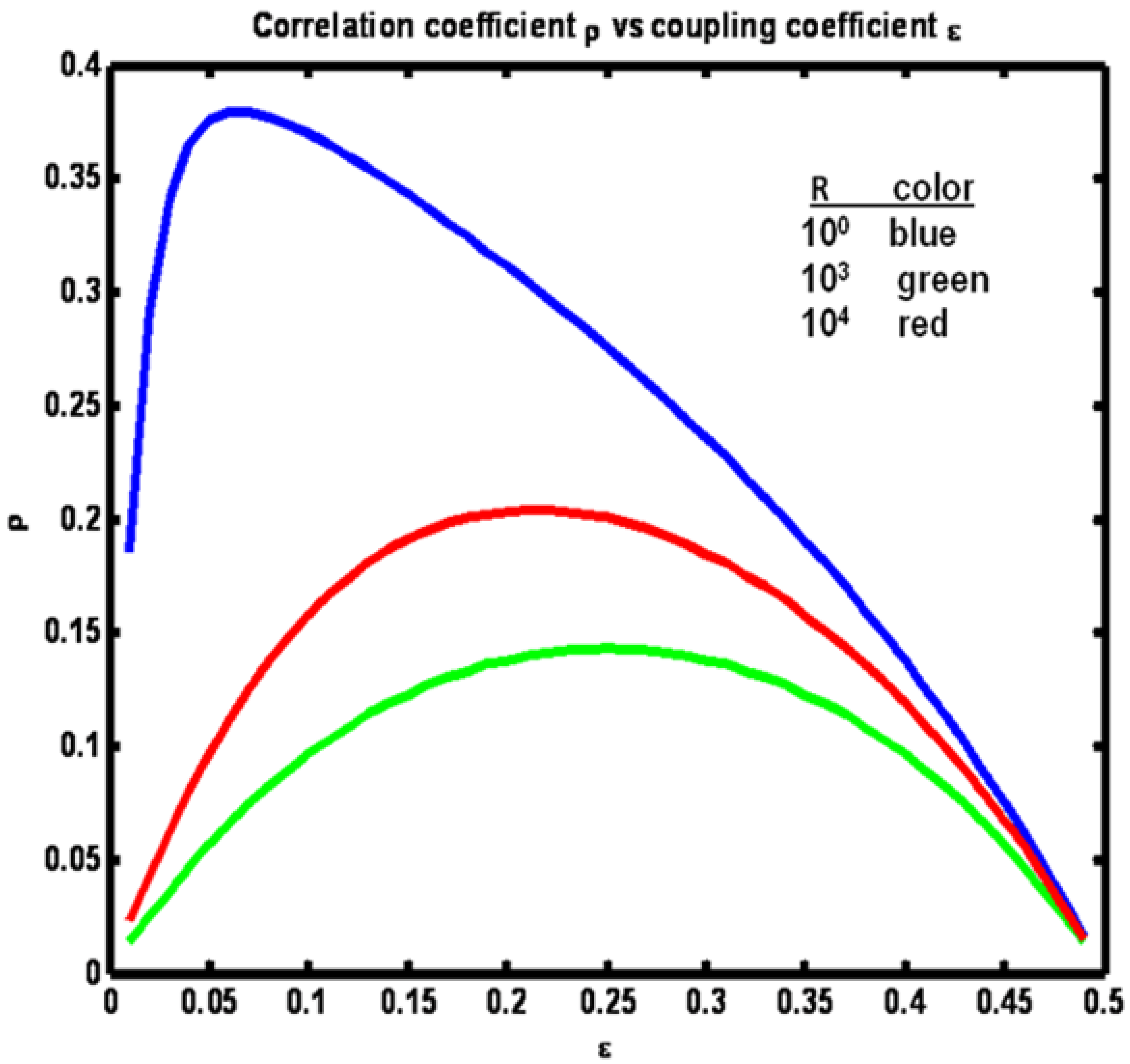
Finally, we consider the sensitivity of the transfer entropies to the coupling term ε. We reprise example system 2 where now ε is varied in the interval (0, ½) and three values of R (somewhat arbitrarily selected to provide visually appealing figures to follow) are considered:
Figure 11 shows the relationship between ρ and ε, where ε
x = ε
y = ε for the three R values. Note that for the case R = Q the relationship is symmetric around ε = ¼. As R departs from equality more correlation between x
n and y
n is obtained.
Figure 11.
Example 2: Correlation coefficient ρ vs coupling coefficient ε for a set of R values (see figure legend).
Figure 11.
Example 2: Correlation coefficient ρ vs coupling coefficient ε for a set of R values (see figure legend).
The reason for this increase is that when the noise driving one process is greater in amplitude than the amplitude of the noise driving the other process, the first process becomes dominant over the other. This domination increases as the disparity between the process noise variances increases (R versus Q). Note also that as the disparity increases, the maximum correlation occurs at increasingly lower values of the coupling term ε. As the disparity increases at fixed ε = ¼ the correlation coefficient ρ increases. However, the variance in the denominator of ρ can be made smaller and thus ρ larger, if the variance of either of the two processes can be reduced. This can be accomplished by reducing ε.
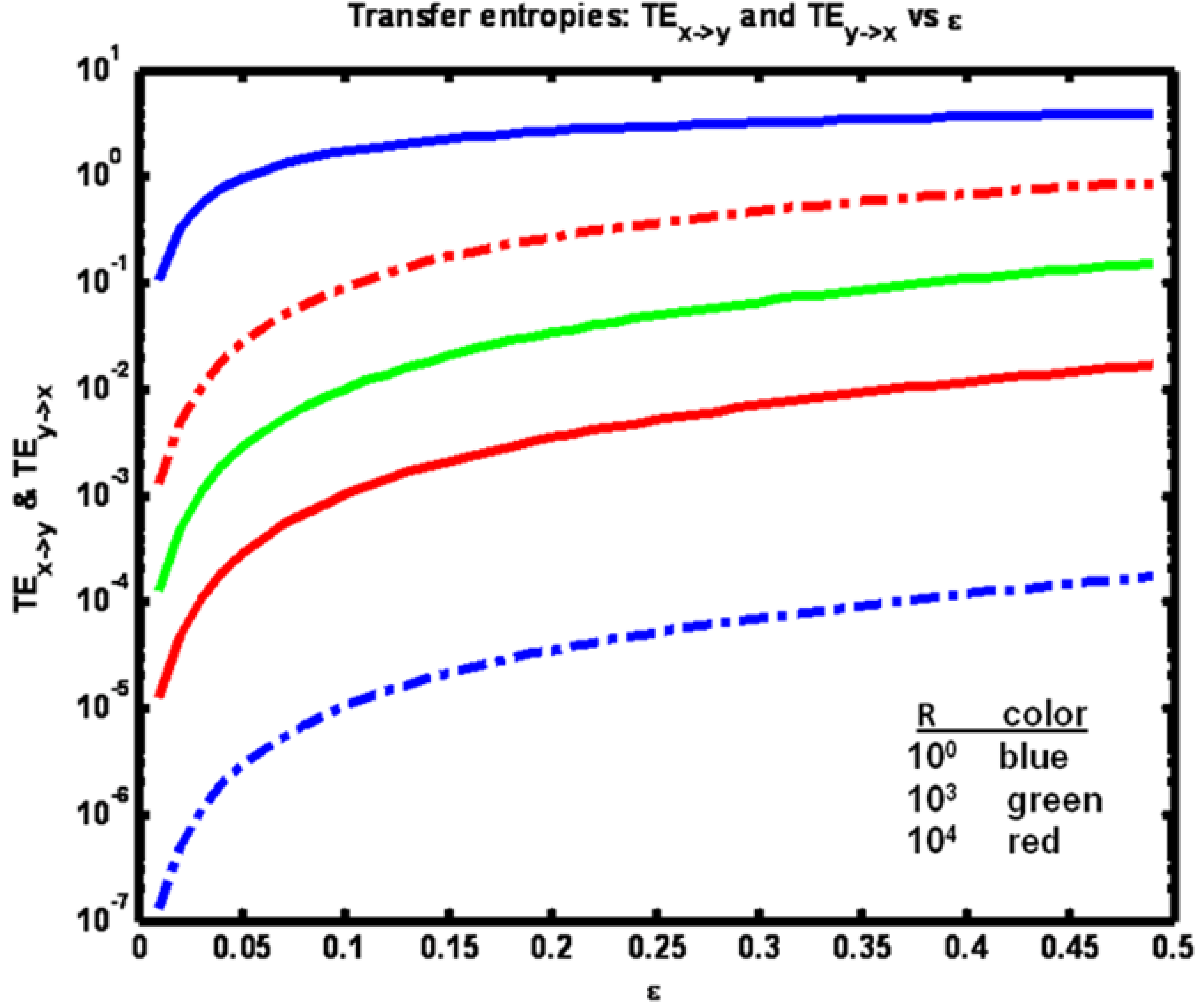
The sensitivities of the transfer entropies to changes in coupling term ε are shown in
Figure 12. Consistent with intuition, all entropies increase with increasing ε. Also, when R < Q (blue trace) we have TE
x‑>y > TE
y‑>x and the reverse for R > Q. (red). For R = Q, TE
x‑>y = TE
y‑>x (green).
Figure 12.
Example 2: Transfer entropies TEx→y (solid lines) vs TEy→x (dashed lines) vs coupling coefficient ε for a set of R values (see figure legend).
Figure 12.
Example 2: Transfer entropies TEx→y (solid lines) vs TEy→x (dashed lines) vs coupling coefficient ε for a set of R values (see figure legend).
Finally, it is interesting to note that whenever we define three cases by fixing Q and varying the setting for R ( one of R1, R2 and R3 for each case) such that R1 < Q, R2 = Q and R3 = Q2/R1 (so that Ri+1 = QRi/R1 for i = 1 and i = 2) we then obtain the symmetric relationships TEx ‑ >y(R1) = TEy ‑ >x(R3) and TEx ‑ >y(R3) = TEy ‑ >x(R1) for all ε in the interval (1, ½). For these cases we also obtain ρ(R1) = ρ(R3) on the same ε interval.
