1. Introduction
One idealized limit for a system of particles is where each particle is totally uncorrelated with all of the others and behaves independently from the rest. Uncorrelated particles have no
a priori preference for any particular region in phase space [
1]. However, totally uncorrelated systems are a physically unattainable limit, because even if the particles were uncorrelated prior to a collision as assumed by Boltzmann’s “molecular chaos” (Stosszahl Ansatz [
2]), their velocities after the collision are no longer truly uncorrelated [
3]; this fact is ultimately responsible for the time-asymmetry that leads to irreversible processes in physical systems. The opposite idealized limit is where every particle is correlated to all the other particles of a system. In all real physical systems, particles have some level of correlation with each other, and the phase space distributions can be very complicated. That is, in general, the particles of a physical system are neither fully correlated nor fully uncorrelated to the other particles of the system.
Systems with no correlations between their particles are in thermal equilibrium - the state where any flow of heat is in balance. Such systems have their distribution functions of velocities stabilized into Maxwell distributions, in the absence of any external force. Space plasmas, however, are non-equilibrium systems that generally reside in stationary states (
i.e., their statistics are temporarily time invariant), but out of thermal equilibrium. These stationary states are described by non-Maxwellian kappa distributions [
4,
5,
6,
7,
8], where the kappa index is inversely proportional to the correlation between the phase space of any two particles [
6].
Debye shielding produces a natural ordering of the correlation of particles in plasmas. Inside a Debye sphere, particles are highly correlated with each other and act together as a single fluid through their electromagnetic interactions. In contrast, at distances greater than a Debye length , particles are largely uncorrelated owing to the Debye shielding of the closer particles. Therefore, each Debye sphere represents a cluster of correlated particles (ions and electrons), which is essentially uncorrelated to the more distant particles and their Debye spheres. In this structuring of particle distributions, clusters share no substantial interaction and behave like essentially uncorrelated phase space elements of the plasma. Particles within a cluster are correlated to each other, but they are essentially uncorrelated to other particles beyond the correlation cluster (Debye sphere).
Below we show how the ordering of particles into correlation clusters by Debye shielding affects the phase space configuration of the plasma and produces a de facto phase space quantization. In particular we, (i) show that the smallest particle energy that can transfer information, , and the correlation lifetime of Debye spheres, , form a special phase space portion , which could quantify a phase space minimum in special cases of space and laboratory plasmas; (ii) examine the constancy of and quantify the values of this phase space portion for several space plasmas that typically reside in stationary states out of thermal equilibrium; (iii) investigate the implications of localized correlation and Debye screening in statistical mechanics; and (iv) examine the consequences of this quantization in modeling the waiting-time distributions of various explosive events, e.g., solar and stellar flares, etc., and other bursts observed in space plasmas; and finally (v) discuss the uniqueness of the value of .
2. Large-Scale Phase Space Quantization
Information about a plasma’s collective properties is transferred beyond the edge of its Debye sphere via wave energy packages that propagate with velocity
. This specific information speed
characterizes the collective character of a plasma, which is related to the correlated electrons and ions in a Debye sphere. There are, of course, numerous different waves and relevant information speeds, some of which are faster than the fast magnetosonic speed, and some of which even reach the speed of light. However, only certain wave modes carry information about the correlated particles in a Debye sphere, as opposed to information about individual particles alone. In space plasmas, this information is typically transferred via fast magnetosonic waves with maximum group velocity equal to the phase velocity
[
9,
10,
11]. Note that
reduces to roughly the Alfvén velocity
for highly magnetized plasmas (low plasma beta), or the sound velocity
(which is often near the thermal speed [
12]) for weakly magnetized plasmas (high beta) [
13].
The particles in collisionless plasmas, such as space plasmas, generally reside in stationary states out of thermal equilibrium [
4,
5,
6,
7,
8]. While the coupling between the particles due to collisions is generally negligible, they do show strong collective behavior owing mainly to wave-particle interactions [
13]. In unmagnetized plasmas, Langmuir and ion-acoustic waves (sound waves) interact with particles as well as some collisions [
14,
15]. In highly magnetized plasmas the magnetic field further binds together the particles in correlated Debye spheres [
16]. In general, plasma electrons and ions are coupled via magnetosonic waves that involve both the magnetic field via the Alfvén speed and the plasma pressure via the sound speed [
15]. Therefore, the Langmuir/ion-acoustic and the triplet of shear Alfvén/slow/fast magnetosonic waves carry information about the correlated particle populations as opposed to information about any one isolated particle alone. Among these, the fast magnetosonic mode has the fastest information speed [
9,
10], with a maximum value given by
[
16]. For this reason, fast magnetosonic shocks form in space plasmas when correlation information tries to propagate faster that the fastest allowable speed [
17]. For example, Coronal Mass Ejections (CMEs) exceeding the fast magnetosonic speed in the solar wind, generate fast magnetosonic forward shocks propagating ahead of them [
18,
19]. Frequently in space plasmas, the Alfvén speed is significantly larger than the sound speed
, and the fast magnetosonic speed reduces to the Alfvén speed,
; in this limit, the Alfvén speed is referred to as the information speed [
11,
12,
20].
Plasma oscillations are implemented through plasmon energy packages with (angular) frequency
; this is approximated by the plasma frequency
when electrons are cold, while
holds in general. Escaping particles may also transfer information, but when their velocities are smaller than
, the waves provide the dominant method for exchanging information. Therefore, information travels at at least the wave velocity,
, and the smallest amount of energy of an ion-electron pair that may escape from the Debye sphere and effectively transfer information is
. Hence, the smallest particle energy that can transfer information is
. We note that the magnetosonic speed does not necessarily connote particle motion at that speed, but instead, implies a minimum limiting speed of a particle that carries information (otherwise the information would be carried by the faster carrier – the waves). (In the above, we use the Debye length
, number of particles in a Debye sphere
, plasma angular frequency
, and sound
and Alfvén
speeds, where
B is the average magnetic field strength and
is the mass density [
13,
15].
and
n are the charge and density of a quasineutral plasma of electrons and monocharged ions with electron and ion mass
,
and temperature
and
;
,
are the reflected mass and temperature;
and
are the permittivity and permeability of the optically isotropic medium.)
The lifetime of a Debye sphere is the characteristic time that particles reside within a Debye length, before leaving because of their thermal motions. This correlation lifetime can be estimated by
, an average length
divided by the thermal speed
, which is a measure of the particles’ outward motion. Due to their thermal motions, individual particles escape and dissolve their correlation with respect to a specific Debye sphere, while at the same time, other, indistinguishable particles from the local region (with a common velocity distribution) enter it. During this continuous escaping and entering of nearby particles, Debye spheres evolve, but their fundamental characteristics remain the same. We note that a given particle may remain in a Debye sphere longer than
, because (i) its motion is not just a linear passage through the sphere, (ii) its speed maybe smaller than
, and/or (iii) it may execute multiple transits inside the Debye sphere. On average, however, particles depart from a Debye sphere travelling ~
owing to their thermal motions. The combination of the smallest particle-energy
and the correlation lifetime
defines a phase space portion, which we denote by
, which may have some special importance as suggested by this study. This is the lower limit for phase space variations that involves (i) energy variations Δ
Ε of the Debye sphere, associated with particle energies
ε that can effectively transfer information,
, and (ii) time intervals that involve the correlation lifetime
; namely:
Note that because
, we derive
, so that the longer the correlation lifetime
, the smaller the plasmon frequency
. We may write this as
, and comparing with (1), we derive
. Therefore, the smallest amount of information energy transferred either by (i) particles,
, or by (ii) waves (plasmons),
, is one and the same. Remarkably, plasmons propagate in energy packages of
, instead of
. According to this equivalence, the particle energy
can be transformed into plasmon energy
, consistent with pressure balance between the particle’s dynamic pressure
and the plasmon energy density
. We conjecture that the same may hold for any particle energy
and plasmon frequency
, so that particle energy
ε can be transferred to plasmon energy package
, following the general relation:
3. Is There Large-Scale Quantization in Non-Equilibrium Plasmas?
Next we examine the constancy of
and quantify the values of
for several space plasmas that are typically out of thermal equilibrium. Debye spheres are similar at nearby locations within a plasma with spatially uniform physical properties. Therefore, it is reasonable to expect that
is a plasma characteristic that has a unique value in any region of a plasma. On the other hand, the phase space value
does not imply any universality between different types of plasmas. Even for the same type of plasma (e.g., solar wind), but with different plasma parameters, Debye spheres might be expected to be characterized by quite different values
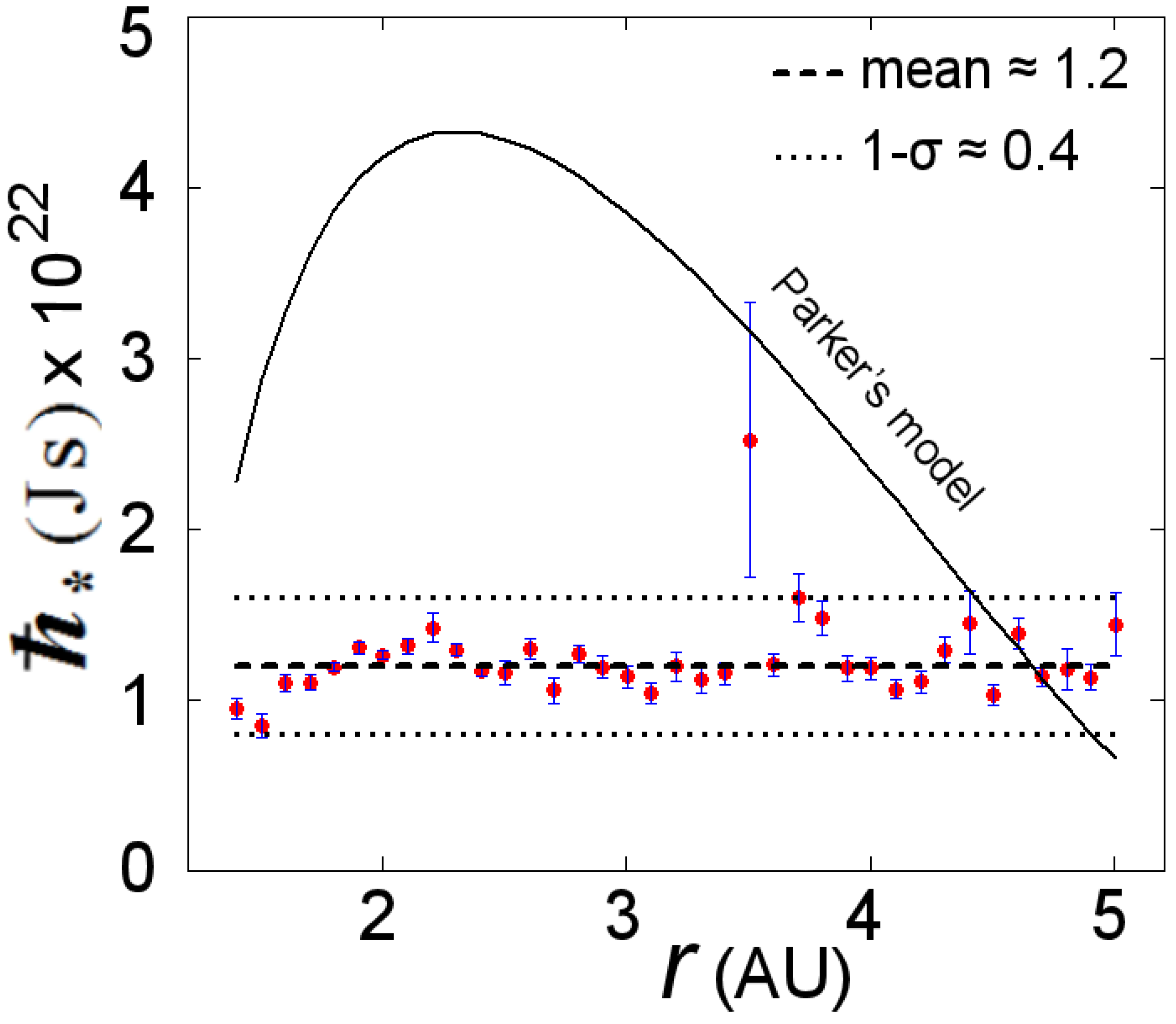
. Ulysses measurements of the solar wind, a largely proton-electron plasma, reveal a quasi-fixed value of
as shown in
Figure 1, even over a broad range of heliocentric distances
and heliolatitudes
ϑ from 80° north to 80° south [
21]. Parker’s relations for solar wind density
n and magnetic field
B expressed in terms of
r and
ϑ, lead to a characteristic variation of values of
over Ulysses orbit. This might be interpreted as the source of the observed quasi-constancy of
; however, in
Appendix A we show that this quasi-constancy is actually independent of Parker’s relations. In particular, we divide the data into 37 small intervals of Ulysses’
r, so that
n and
B have variations independent of Parker’s relations and show that
has similar values for each of these intervals. Thus
is characterized by a quasi-constant value, which clearly deviates from the variation expected from Parker’s relations.
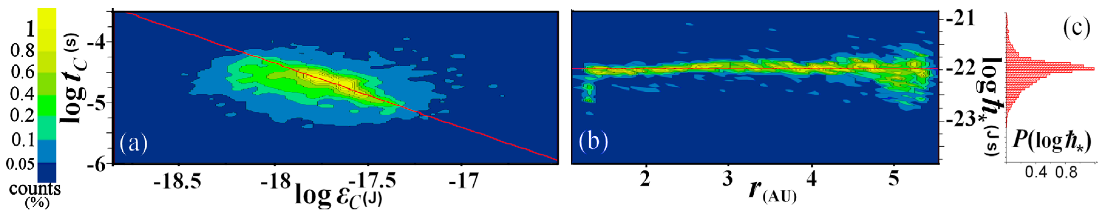
Figure 1.
Phase space portion
calculated for the solar wind ion-electron plasma measurements and using Equation (1). (
a) Diagram
(on a log-log scale), constructed from Ulysses daily measurements. (
b) The product
is depicted as a function of heliocentric distance
r. (a) and (b) are two-dimensional normalized histograms. (
c) Normalized histogram of the values of the values of
. The fitted line in (a) has slope -1 and intercept
(=
). The weighted mean of
values in (b) is found to be
. (For details on the statistical method, see
Appendix A).
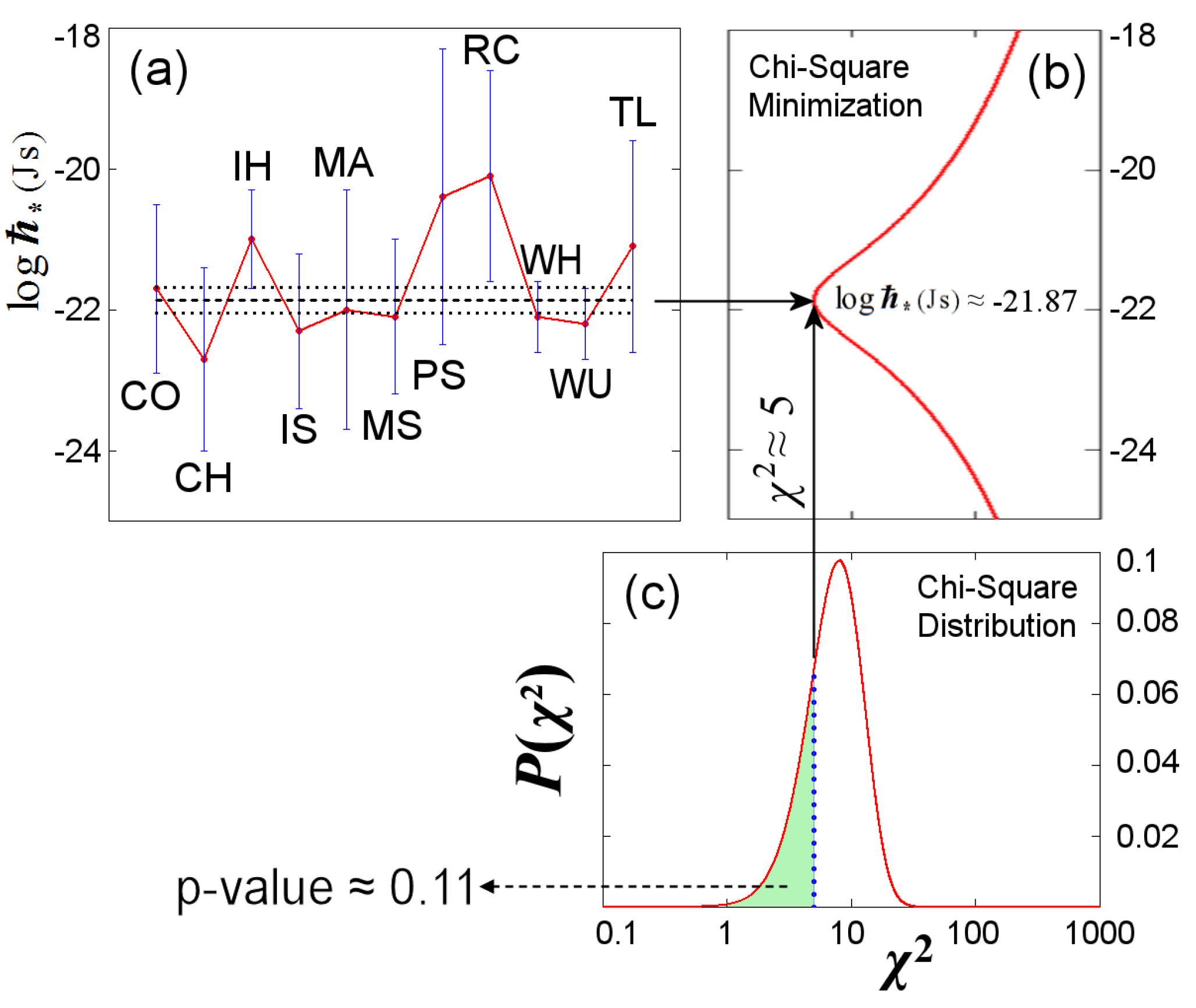
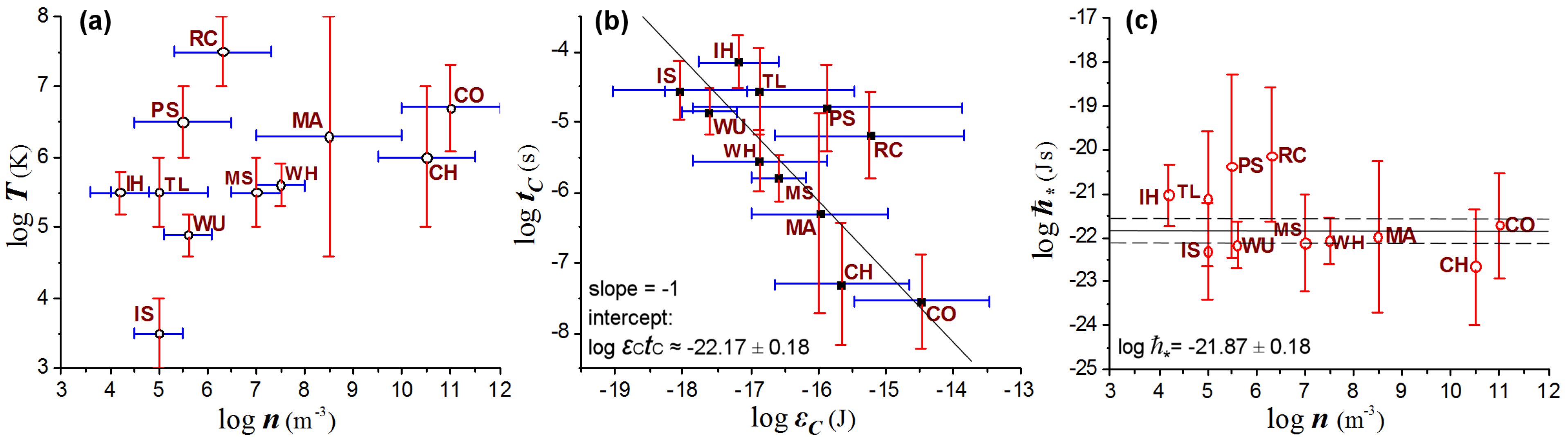
Figure 2.
Phase space portion
in non-equilibrium space plasmas. (
a) Types of space plasmas that are typically out of thermal equilibrium, across a broad range of electron density and temperature. (
b) These plasmas produce a linear relation in
diagram (log-log scale) with slope -1, implying a relation
constant. (
c) The constancy of
is also indicated by the respective log
values. (For details on the statistical method, see
Appendix B. Details of plasma parameters used are provided in the
Appendix C. Acronyms: CH: Corona Holes; CO: Corona; IH: Inner Heliosheath; IS: Interstellar; MA: Magnetosphere; MS: Magnetosheath; PS: Plasma Sheet; RC: Ring Current; TL: Tail Lobe; WH: solar Wind - Helios; WU: solar Wind-Ulysses).
Remarkably, a similar value of
found for the Ulysses observations appears to characterize not only the solar wind, but also many other space plasmas that are typically in stationary states out of thermal equilibrium [
4,
5,
6,
7,
8], as shown in
Figure 2. The weighted mean value of
derived from the statistical analysis of these data corresponds to
, while the statistical hypothesis of a constant
is highly likely (p-value ~ 0.11; see
Appendix B).
4. Statistical Mechanics of Non-Equilibrium Plasmas
In this section we investigate the implications of localized correlation and Debye screening for the statistical mechanics of non-equilibrium plasmas. The statistical treatment of phase space with correlation clusters (Debye spheres) is fundamentally different from that of the classical case, which assumes uncorrelated particles. However, it can be thought of in a similar way to the classical case, but with the essentially uncorrelated clusters (owing to Debye screening) replacing the assumed-to-be uncorrelated particles in Boltzmann-Gibbs statistics.
For systems with no correlation, the number of microstates in an infinitesimal volume of
N-particle phase space is given by
, or expressed in terms of the dimensionless thermal parameter
σ,
, where
;
N is the total number of particles,
L the system’s dimensions,
m,
T, and
are the particle mass, temperature, and characteristic thermal speed [
6]. At thermal equilibrium, the entropy is given by the Sackur-Tetrode equation
, where the non-negativity of entropy implies the thermal parameter
σ to be constrained by
.
For plasmas with clusters of correlated particles, is constant across regions with uniform physical properties; hence, the microstates are obtained by dividing the phase space by instead of (with ), where the factor stands for all the possible ways of having N undistinguished particles within uncorrelated clusters, i.e., , for ; is the number of correlated particles in the mth uncorrelated cluster, with average . Replacing h with , we obtain the thermal parameter . For quasineutral plasmas of ions and electrons, the thermal parameter is that can be written as .
The entropy formulation for systems out of thermal equilibrium is unknown. It is also unknown if this entropic formulation can be defined for any possible (stationary or non-stationary) state in which a system may reside. However, no matter how complex this general formulation is, it has to be analytically definable at thermal equilibrium. There, the generalized entropy is reduced to the Sackur-Tetrode equation that requires the constraint
. The limit of
has different meaning for systems with or without correlations:
- (1)
For systems with no correlations, the limit means the system approaches "quantum degeneracy", beyond which the non-quantum approach of Statistical Mechanics is no longer valid. This concept is usually described by comparing the thermal de Broglie wavelength and the inter-particle distance : The passage of the system into the quantum regime implies or .
- (2)
For systems with correlations, the limit means the system transitions to "correlation degeneracy", beyond which the description through correlation clusters (Debye spheres) no longer applies. Then, the correlation clusters dissolve and the entropy increases, leading to plasma states that involve less-significant correlations.
The value of
can be derived by applying the condition
in plasmas using the assumption that systems exhibiting explosive events are in correlation degeneracy. For example, the solar corona plasma that is associated with solar flares emissions could be such a plasma. Given the formulation of thermal parameter, we derive
or
for
(units are in SI). For the solar corona we have
and
(
Appendix C), from which we calculate
, consistent with the other values of
found above.
5. Waiting-Time Distributions of Explosive Events in Non-Equilibrium Space Plasmas
Explosive events (also called explosive instabilities or bursts) are poorly understood and yet occur in a variety of space plasmas (e.g., solar and stellar flares, coronal mass ejections, magnetospheric substorms,
etc.). Various mechanisms have been proposed for different types of events, but there is no agreement between them, and thus each one may be driven by different causes (e.g., see [
22]). Here we consider if correlation degeneracy might provide a “phenomenological” description of bursts, independent of their unique causes or triggers.
The waiting-time distribution of bursts in space plasmas can be modeled via Equation (2) and the one-particle energy distribution for a correlated particle in a Debye sphere. This energy is transferred to plasmons, the particles that propagate fluctuations in plasmas. In particular, the frequency
of a burst in a plasma is reasonably proportional to both the plasmon frequency
and the expansion rate within the plasma that is given by the collision frequency
normalized over the plasma’s natural frequency
[
15],
i.e.,
. When the plasmons propagate with the plasma frequency
, the burst frequency is simply approximated by the collision frequency, while in general, burst and plasmon frequencies have associated distributions. Then, the waiting-time between successive bursts is given by
. Given Eq.(2), the distribution of the burst waiting-times
can be associated with the one-particle distribution of energy
,
i.e.,
or
where the characteristic time
τ can be used to derive the value of
, given the values of
T and
n (or
ND). Substituting the Coulomb collision rate
[
15] in Eq. (3a), we find,
with units
(
),
τ (h),
T (MK), and
ND (
).
The whole energy distribution
includes the energy density of states
, so that
, where
P is the energy distribution without energy density
. For instance,
P may be the BG distribution for systems at thermal equilibrium, or the kappa distribution for systems in stationary states out of thermal equilibrium [
4,
5,
6,
7,
8]. In general, the distribution
P is constant at low energy, and thus, does not affect the whole distribution,
i.e.,
. Low energy corresponds to large waiting-times in the tail of their distribution. Hence, Eq. (3a) gives
~
(for
with
f indicating the system’s dimensionality); therefore, the asymptotic behavior of the waiting-time distribution is
(for
f=3). This result has already been shown for several different types of bursts such as Solar Flares (SoFs), Coronal Mass Ejections (CMEs), and Stellar Flares (StFs), as document in
Table 1 [
23,
24,
25,
26,
27]. This power-law behavior with slope ~2.5 is far from the exponential-law that is expected from a local Poisson process; interestingly, the Poisson hypothesis is not consistent with observations [
25]. Even a time-dependent Poisson process [
28] cannot give the exact profile of the observed waiting-time distributions that exhibit a maximum and a tail with a power-law asymptotic behavior. In contrast, given the large phase space quantization
and the kappa distribution of energy [
6], the resulting burst waiting-time distribution is:
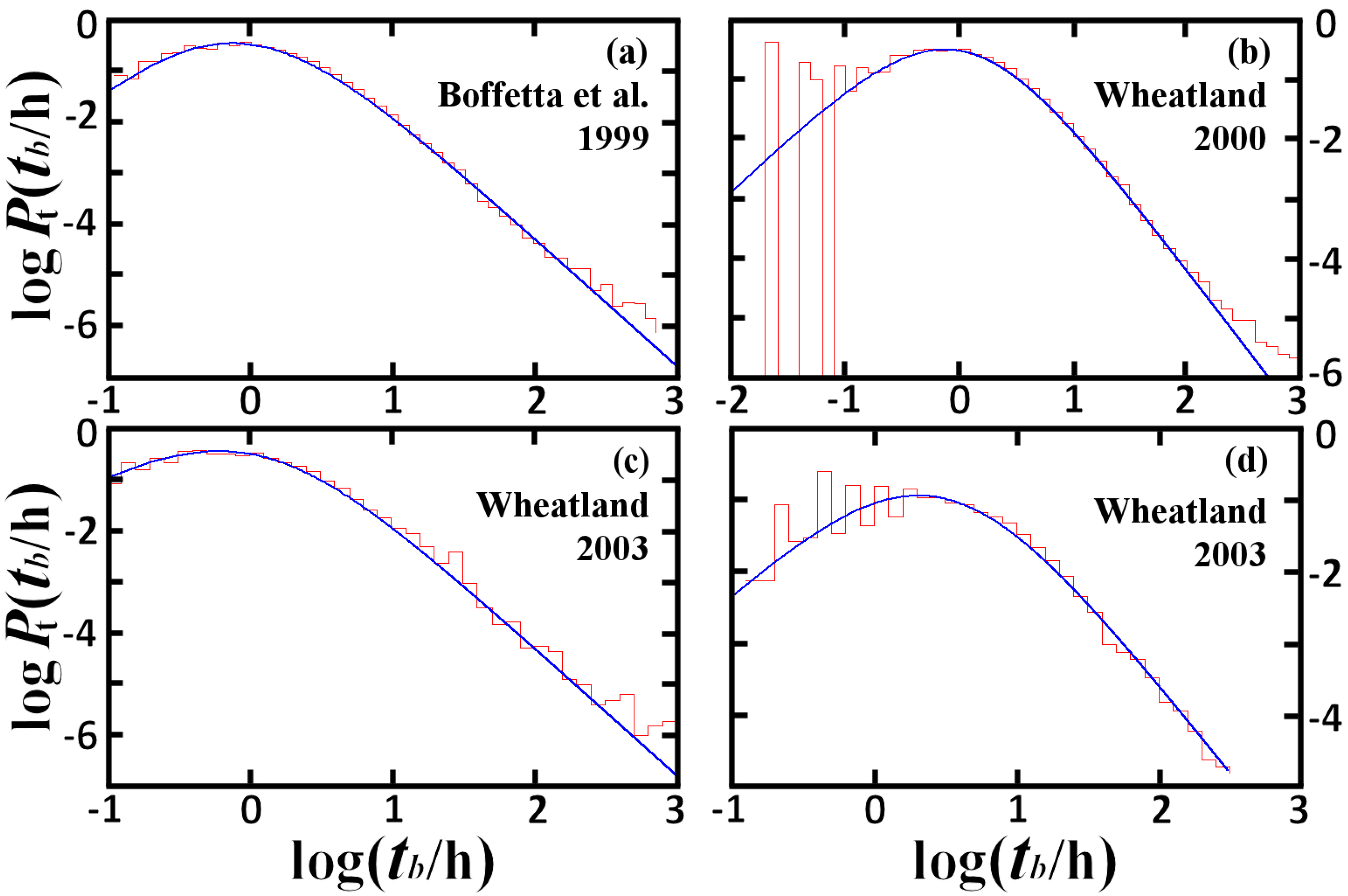
with a maximum at
. This derived distribution closely matches the observational waiting-time distributions of solar flares (
τ = 1.85 ± 0.05 [
23],
τ = 1.85 ± 0.05 [
28];
τ = 1.50 ± 0.10 [
26]; their weighted mean is shown in
Table 2) and CMEs (
τ = 5.0 ± 0.5 [
26]), shown in
Figure 3. This procedure leads to a particular value of
for various plasma sources of bursts (SoFs [
23,
26,
28], CMEs [
26], Geomagnetic Substorms (GSs) [
29];
Table 2).
Table 1.
Power Law in Waiting-Time Distributions in Space Plasmas with Bursts.
Table 1.
Power Law in Waiting-Time Distributions in Space Plasmas with Bursts.
| Bursts | Refs | slope |
|---|
| SoFs | [23,24] | −2.38 ± 0.03; −2.40 ± 0.10 |
| SoFs | [25] | −2.38 ± 0.06 |
| SoFs | [26] | −2.26 ± 0.11 |
| CMEs | [26] | −2.36 ± 0.11 |
| StFs | [27] | −2.29 ± 0.07; −2.31 ± 0.12 |
Table 2.
Estimation of in Space Plasmas with Bursts.
Table 2.
Estimation of in Space Plasmas with Bursts.
| Bursts | Refs | τ (h) | Plasma | log T(K) | log ND | |
|---|
| SoFs | [23,26,28] | 1.81 ± 0.03 | (CO) | 6.7 ± 0.6 | 10.2 ± 1.0 | −22.72 ± 1.17 |
| CMEs | [26] | 5.0 ± 0.5 | (CH) | 6.0 ± 1.0 | 9.4 ± 1.6 | −22.21 ± 1.89 |
| GSs | [29] | 5.5 ± 0.5 | (MA) | 6.3 ± 1.7 | 10.9 ± 2.7 | −23.31 ± 3.14 |
Figure 3.
Waiting-time distributions of (
a–c) Solar Flares [
23,
26,
28], and (
d) CMEs [
26] (red data). The modeled distribution (blue lines) that is derived from (3) using one-particle kappa distribution of energy is well-fitted to the data (over six orders of magnitude), leading to an estimation of
consistent with other methods.
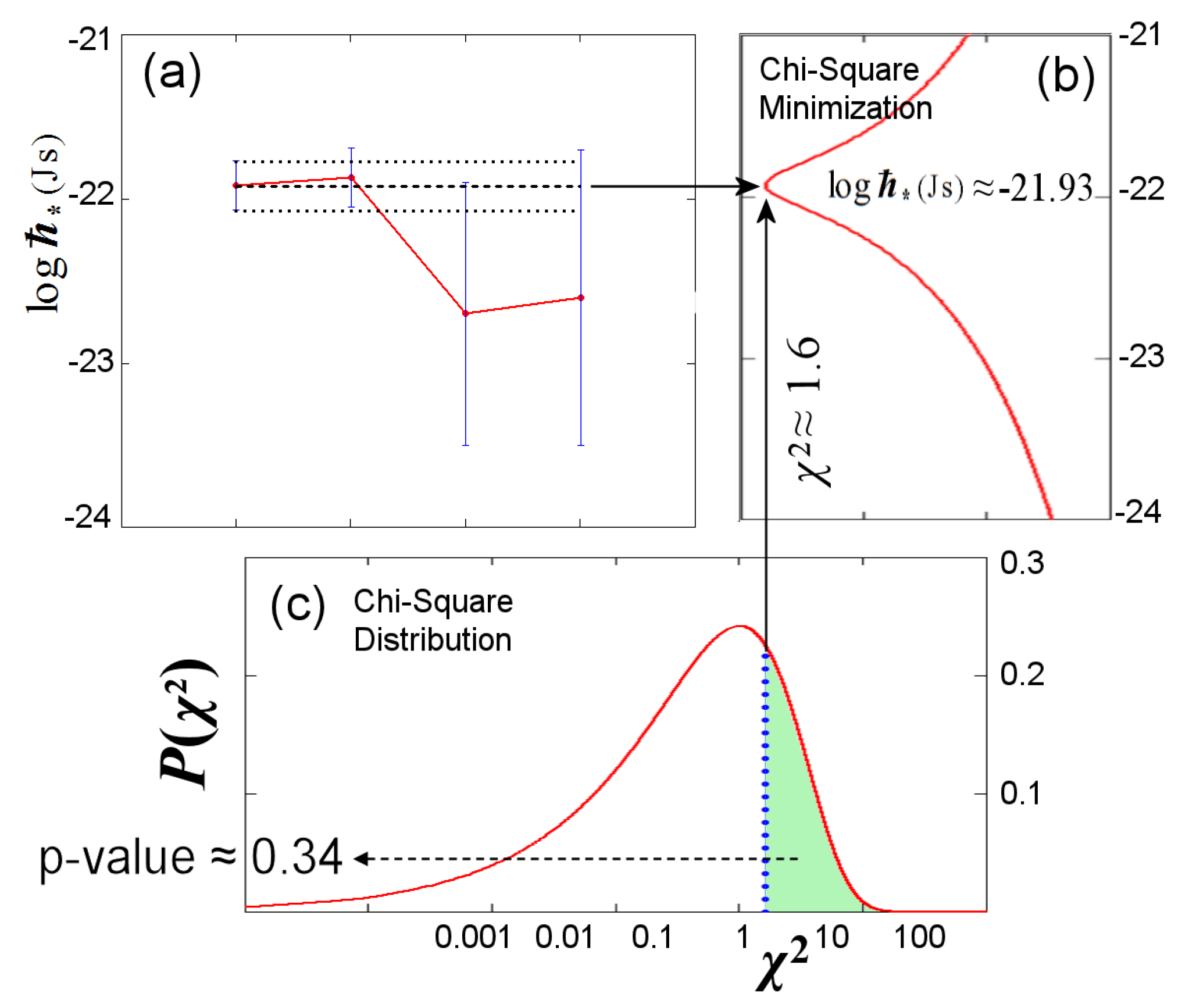
6. Conclusions
In this study, we identify a phase space minimum
that characterizes many non-equilibrium space plasmas and appears to have quasi-constant value some 12 orders of magnitude larger than the fundamental Planck constant. We used four independent methods (1) Ulysses solar wind measurements, (2) space plasmas that typically reside in stationary states out of thermal equilibrium and spanning a broad range of physical properties, (3) an entropic limit emerging from statistical mechanics, (4) waiting-time distributions of explosive events in space plasmas, to calculate values of
as described above and summarized in
Table 3. The weighted mean of
or
corresponds to the non-reduced value
or
.
Table 3.
Four Different Methods of Estimation.
Table 3.
Four Different Methods of Estimation.
| Method | |
|---|
| Ulysses measurements (Figure 1) | −21.92 ± 0.15 |
| Non-equilibrium space plasmas (Figure 2) | −21.87 ± 0.18 |
| Correlation Degeneracy | −22.7 ± 0.8 |
| Bursts (Table 2, Figure 3) | −22.6 ± 0.9 |
| Weighted Mean (Appendix B) | −21.93 ± 0.14 |
It is important to remember that the general formulation of the phase space portion
in (1) does not imply any specific value, and thus any value of
might be possible. Remarkably, the various derived values of
are very consistent. This consistency suggests the possibility that this value may be some sort of general physical constant at least for many plasmas in stationary states out of thermal equilibrium. While some of the uncertainty in its values (
Table 3) are surely due to inaccuracies of the methods, it is also possible that
has close but still different values for different plasmas. It is interesting to note that such a quasi-constancy could also conceivably characterize the Planck constant, where the two most accurate methods for determining its value,
i.e., watt balance [
30,
31,
32] and the X-ray crystal density [
33], do not agree with one another to within their stated uncertainties; their difference in
h is
while the uncertainties are significantly smaller,
i.e.,
and
. In addition, further future experimentation may find evidence of violations of the time [
34] and position invariance of Planck constant [
35].
Both the plasma
and Planck
h quantify types of minimum possible phase space portions. We note that a minimum possible phase space portion also characterizes phase space variations, namely, the phase space cannot vary in portions smaller than this minimum; hence, similar to
h, we refer to this
as phase space quantization, but on a much larger scale. While
h characterizes a general quantization of physical systems, we have so far only shown
to apply to a range of non-equilibrium space plasmas, where Debye screening produces localized correlation [
6]. However, other physical processes may also produce localized correlations, thus, we speculate that other physical systems of correlated particles might also exhibit a similar phase space quantization. We anticipate the current study to be a starting point for sophisticated analyses of the large scale phase space quantization
in plasmas and beyond. The existence of a second phase space quantization for a variety of plasmas, similar to the classical Planck constant but 12 orders of magnitude larger, may be revealing a new and fundamental property of many plasmas and correlated systems more generally.


