Generalized (c,d)-Entropy and Aging Random Walks

Abstract

Complex systems are often inherently non-ergodic and non-Markovian and Shannon entropy loses its applicability. Accelerating, path-dependent and aging random walks offer an intuitive picture for non-ergodic and non-Markovian systems. It was shown that the entropy of non-ergodic systems can still be derived from three of the Shannon–Khinchin axioms and by violating the fourth, the so-called composition axiom. The corresponding entropy is of the form $S_{c,d}\sim {\sum }_i\Gamma (1+d,1-cln{p}_i)$ and depends on two system-specific scaling exponents, c and d. This entropy contains many recently proposed entropy functionals as special cases, including Shannon and Tsallis entropy. It was shown that this entropy is relevant for a special class of non-Markovian random walks. In this work, we generalize these walks to a much wider class of stochastic systems that can be characterized as “aging” walks. These are systems whose transition rates between states are path- and time-dependent. We show that for particular aging walks, $S_{c,d}$ is again the correct extensive entropy. Before the central part of the paper, we review the concept of $(c,d)$-entropy in a self-contained way.

1. Introduction: Mini-Review of $(c,d)$-Entropy

In their seminal works, Shannon and Khinchin showed that, assuming four information theoretic axioms, the entropy must be of the Boltzmann–Gibbs type, $S=-{\sum }_i{p}_{i}log{p}_i$. In many physical systems, one of these axioms may be violated. For non-ergodic systems, the so-called separation axiom (Shannon–Khinchin Axiom 4) is not valid. We show that whenever this axiom is violated, the entropy takes a more general form, $S_{c,d}\propto {\sum }_i^W\Gamma (d+1,1-clog{p}_i)$, where c and d are scaling exponents and $\Gamma (a,b)$ is the incomplete gamma function. These exponents $(c,d)$ define equivalence classes for all, interacting and non-interacting, systems and unambiguously characterize any statistical system in its thermodynamic limit. The proof is possible because of two newly discovered scaling laws, which exist for any entropic form, given the first three Shannon–Khinchin axioms hold [1]. $(c,d)$ can be used to define equivalence classes of statistical systems. A series of known entropies can be classified in terms of these equivalence classes. We show that the corresponding distribution functions are special forms of Lambert-$\mathcal{W}$ exponentials containing, as special cases, Boltzmann, stretched exponential and Tsallis distributions (power-laws). We go on by showing how the dependence of phase space volume $W\left(N\right)$ of a classical system on its size N uniquely determines its extensive entropy and, in particular, the requirement extensively fixes the exponents $(c,d)$ [2]. We give a concise criterion when this entropy is not of the Boltzmann–Gibbs–Shannon type, but has to assume a generalized (non-additive) form. We showed that generalized entropies can only exist when the dynamically (statistically) relevant fraction of degrees of freedom in the system vanishes in the thermodynamic limit [2]. These are systems where the bulk of the degrees of freedom is frozen and is practically statistically inactive. Systems governed by generalized entropies are therefore systems whose phase space volume effectively collapses to a lower-dimensional “surface”. We explicitly illustrated the situation for binomial processes and argue that generalized entropies could be relevant for self-organized critical systems, such as sand piles, for spin systems that form meta-structures, such as vortices, domains, instantons, etc., and for problems associated with anomalous diffusion [2]. In this contribution, we largely follow the lines of thought presented in [1,2,3].

Theorem 2 in the seminal 1948 paper, The Mathematical Theory of Communication [4], by Claude Shannon, proves the existence of the one and only form of entropy, given that three fundamental requirements hold. A few years later, A.I. Khinchin remarked in his Mathematical Foundations of Information Theory [5]: “However, Shannon’s treatment is not always sufficiently complete and mathematically correct so that, besides having to free the theory from practical details, in many instances I have amplified and changed both the statement of definitions and the statement of proofs of theorems.” Khinchin adds a fourth axiom. The three fundamental requirements of Shannon, in the “amplified” version of Khinchin, are known as the Shannon–Khinchin (SK) axioms. These axioms list the requirements needed for an entropy to be a reasonable measure of the “uncertainty” about a finite probabilistic system. Khinchin further suggests to also use entropy as a measure of the information gained about a system when making an “experiment”, i.e., by observing a realization of the probabilistic system.

• Khinchin’s first axiom states that for a system with W potential outcomes (states), each of which is given by a probability, $p_i\ge 0$, with ${\sum }_{i=1}^W{p}_i=1$, the entropy, $S(p_1,\cdots ,p_W)$, as a measure of uncertainty about the system must take its maximum for the equi-distribution $p_i=1/W$, for all i.
• Khinchin’s second axiom (missing in [4]) states that any entropy should remain invariant under adding zero-probability states to the system, i.e., $S(p_1,\cdots ,p_W)=S(p_1,\cdots ,p_W,0)$.
• Khinchin’s third axiom (separability axiom) finally makes a statement of the composition of two finite probabilistic systems, A and B. If the systems are independent of each other, entropy should be additive, meaning that the entropy of the combined system, $A+B$, should be the sum of the individual systems, $S\left(A+B\right)=S\left(A\right)+S\left(B\right)$. If the two systems are dependent on each other, the entropy of the combined system, i.e., the information given by the realization of the two finite schemes, A and B, $S(A+B)$, is equal to the information gained by a realization of system A, $S\left(A\right)$, plus the mathematical expectation of information gained by a realization of system B, after the realization of system A, ${S\left(A+B\right)=S\left(A\right)+S|}_A\left(B\right)$.
• Khinchin’s fourth axiom is the requirement that entropy is a continuous function of all its arguments, $p_i$, and does not depend on anything else.

Given these axioms, the Uniqueness Theorem [5] states that the one and only possible entropy is

$$S(p_1,\cdots ,p_W)=-k\sum _{i=1}^W{p}_{i}log{p}_i$$

(1)

where k is an arbitrary positive constant. The result is, of course, the same as Shannon’s. We call the combination of four axioms the Shannon–Khinchin (SK) axioms.

From information theory, we now move to physics, where systems may exist that violate the separability axiom. This might especially be the case for non-ergodic, complex systems exhibiting long-range and strong interactions. Such complex systems may show extremely rich behavior in contrast to simple ones, such as gases. There exists some hope that it should be possible to understand such systems also on a thermodynamical basis, meaning that a few measurable quantities would be sufficient to understand their macroscopic phenomena. If this were possible, through an equivalent to the second law of thermodynamics, some appropriate entropy would enter as a fundamental concept relating the number of microstates in the system to its macroscopic properties. Guided by this hope, a series of so-called generalized entropies have been suggested over the past few decades; see [6,7,8,9,10,11] and Table 1. These entropies have been designed for different purposes and have not been related to a fundamental origin. Here, we ask how generalized entropies can look if they fulfill some of the Shannon–Khinchin axioms, but explicitly violate the separability axiom. We do this axiomatically, as first presented in [1]. By doing so, we can relate a large class of generalized entropies to a single fundamental origin.

The reason why this axiom is violated in some physical, biological or social systems is broken ergodicity, i.e., that not all regions in the phase space are visited, and many microstates are effectively “forbidden”. Entropy relates the number of microstates of a system to an extensive quantity, which plays the fundamental role in the systems thermodynamical description. Extensive means that if two initially isolated, i.e., sufficiently separated systems, A and B, with $W_A$ and $W_B$ the respective numbers of states, are brought together, the entropy of the combined system, $A+B$, is $S\left(W_{A+B}\right)=S\left(W_A\right)+S\left(W_B\right)$. $W_{A+B}$ is the number of states in the combined system, $A+B$. This is not to be confused with additivity, which is the property that $S\left(W_A{W}_B\right)=S\left(W_A\right)+S\left(W_B\right)$. Both extensivity and additivity coincide if the number of states in the combined system is $W_{A+B}=W_A{W}_B$. Clearly, for a non-interacting system, Boltzmann–Gibbs–Shannon entropy, $S_{\mathrm{BGS}}\left[p\right]=-{\sum }_i^W{p}_{i}ln{p}_i$, is extensive and additive. By “non-interacting” (short-range, ergodic, sufficiently mixing, Markovian, etc.) systems, we mean $W_{A+B}=W_A{W}_B$. For interacting statistical systems, the latter is in general not true; the phase space is only partly visited, and $W_{A+B}<W_A{W}_B$. In this case, an additive entropy, such as Boltzmann–Gibbs–Shannon, can no longer be extensive and vice versa. To ensure the extensivity of entropy, an entropic form should be found for the particular interacting statistical systems at hand. These entropic forms are called generalized entropies and usually assume trace form [6,7,8,9,10,11]

$$S_g\left[p\right]=\sum _{i=1}^{W}g\left(p_i\right)$$

(2)

W being the number of states. Obviously not all generalized entropic forms are of this type. Rényi entropy, for example, is of the form, $G({\sum }_i^{W}g\left(p_i\right))$, with G a monotonic function. We use trace forms Equation (2) for simplicity. Rényi forms can be studied in exactly the same way, as will be shown, however, at more technical cost.

Table 1. Order in the zoo of recently introduced entropies for which SK1–SK3 hold. All of them are special cases of the entropy given in Equation (3), and their asymptotic behavior is uniquely determined by c and d. It can be seen immediately that $S_{q>1}$, $S_b$ and $S_E$ are asymptotically identical; so are $S_{q<1}$ and $S_{\kappa }$, as well as $S_{\eta }$ and $S_{\gamma }$.

Entropy		c	d	Reference
$S_{c,d}=er{\sum }_i\Gamma (d+1,1-cln{p}_i)-cr$	$(r={(1-c+cd)}^{-1})$	c	d
$S_{BGS}={\sum }_i{p}_{i}ln(1/p_i)$		1	1	[5]
$S_{q<1}\left(p\right)=\frac{1-\sum p_i^q}{q-1}$	$(q<1)$	$c=q<1$	0	[6]
$S_{\kappa }\left(p\right)=-{\sum }_i{p}_i\frac{p_i^{\kappa }-p_i^{-\kappa }}{2\kappa }$	($0<\kappa \le 1$)	$c=1-\kappa$	0	[8]
$S_{q>1}\left(p\right)=\frac{1-\sum p_i^q}{q-1}$	$(q>1)$	1	0	[6]
$S_b\left(p\right)={\sum }_i(1-e^{-b{p}_i})+e^{-}b-1$	$(b>0)$	1	0	[9]
$S_E\left(p\right)={\sum }_i{p}_i(1-e^{\frac{p_i-1}{p_i}})$		1	0	[10]
$S_{\eta }\left(p\right)={\sum }_i\Gamma (\frac{\eta +1}{\eta },-ln{p}_i)-p_i\Gamma \left(\frac{\eta +1}{\eta }\right)$	$(\eta >0)$	1	$d=\frac{1}{\eta }$	[7]
$S_{\gamma }\left(p\right)={\sum }_i{p}_i{ln}^{1/\gamma }(1/p_i)$		1	$d=1/\gamma$	[12,13]
$S_{\beta }\left(p\right)={\sum }_i{p}_i^{\beta }ln(1/p_i)$		$c=\beta$	1	[14]

Table 1. Order in the zoo of recently introduced entropies for which SK1–SK3 hold. All of them are special cases of the entropy given in Equation (3), and their asymptotic behavior is uniquely determined by c and d. It can be seen immediately that $S_{q>1}$, $S_b$ and $S_E$ are asymptotically identical; so are $S_{q<1}$ and $S_{\kappa }$, as well as $S_{\eta }$ and $S_{\gamma }$.

Entropy		c	d	Reference
$S_{c,d}=er{\sum }_i\Gamma (d+1,1-cln{p}_i)-cr$	$(r={(1-c+cd)}^{-1})$	c	d
$S_{BGS}={\sum }_i{p}_{i}ln(1/p_i)$		1	1	[5]
$S_{q<1}\left(p\right)=\frac{1-\sum p_i^q}{q-1}$	$(q<1)$	$c=q<1$	0	[6]
$S_{\kappa }\left(p\right)=-{\sum }_i{p}_i\frac{p_i^{\kappa }-p_i^{-\kappa }}{2\kappa }$	($0<\kappa \le 1$)	$c=1-\kappa$	0	[8]
$S_{q>1}\left(p\right)=\frac{1-\sum p_i^q}{q-1}$	$(q>1)$	1	0	[6]
$S_b\left(p\right)={\sum }_i(1-e^{-b{p}_i})+e^{-}b-1$	$(b>0)$	1	0	[9]
$S_E\left(p\right)={\sum }_i{p}_i(1-e^{\frac{p_i-1}{p_i}})$		1	0	[10]
$S_{\eta }\left(p\right)={\sum }_i\Gamma (\frac{\eta +1}{\eta },-ln{p}_i)-p_i\Gamma \left(\frac{\eta +1}{\eta }\right)$	$(\eta >0)$	1	$d=\frac{1}{\eta }$	[7]
$S_{\gamma }\left(p\right)={\sum }_i{p}_i{ln}^{1/\gamma }(1/p_i)$		1	$d=1/\gamma$	[12,13]
$S_{\beta }\left(p\right)={\sum }_i{p}_i^{\beta }ln(1/p_i)$		$c=\beta$	1	[14]

Let us revisit the Shannon–Khinchin axioms in the light of generalized entropies of trace form Equation (2). Specifically, Axioms SK1–SK3 (now re-ordered) have implications on the functional form of g.

• SK1: The requirement that S depends continuously on p implies that g is a continuous function.
• SK2: The requirement that the entropy is maximal for the equi-distribution $p_i=1/W$ (for all i) implies that g is a concave function.
• SK3: The requirement that adding a zero-probability state to a system, $W+1$ with $p_{W+1}=0$, does not change the entropy implies that $g\left(0\right)=0$.
• SK4 (separability axiom): The entropy of a system, composed of sub-systems A and B, equals the entropy of A plus the expectation value of the entropy of B, conditional on A. Note that this also corresponds exactly to Markovian processes.

As mentioned, if SK1 to SK4 hold, the only possible entropy is the Boltzmann–Gibbs–Shannon (BGS) entropy. We are now going to derive the extensive entropy when separability Axiom SK4 is violated. Obviously, this entropy will be more general and should contain BGS entropy as a special case.

We now assume that Axioms SK1, SK2, SK3 hold, i.e., we restrict ourselves to trace form entropies with g continuous, concave and $g\left(0\right)=0$. These systems we call admissible systems. Admissible systems when combined with a maximum entropy principle show remarkably simple mathematical properties [15,16].

This generalized entropy for (large) admissible statistical systems (SK1–SK3 hold) is derived from two hitherto unexplored fundamental scaling laws of extensive entropies [1]. Both scaling laws are characterized by exponents c and d, respectively, which allow one to uniquely define equivalence classes of entropies, meaning that two entropies are equivalent in the thermodynamic limit if their exponents $(c,d)$ coincide. Each admissible system belongs to one of these equivalence classes $(c,d)$, [1].

In terms of the exponents $(c,d)$, we showed in [1] that all generalized entropies have the form

$$S_{c,d}\propto \sum _i^W\Gamma (d+1,1-clog{p}_i)$$

(3)

with $\Gamma (a,b)={\int }_b^{\infty }dt{t}^{a-1}exp(-t)$ the incomplete Gamma-function.

Special Cases of Equivalence Classes

Let us look at some specific equivalence classes $(c,d)$.

• Boltzmann–Gibbs entropy belongs to the $(c,d)=(1,1)$ class. One gets from Equation (3)

  $$S_{1,1}\left[p\right]=\sum _i{g}_{1,1}\left(p_i\right)=-\sum _i{p}_{i}ln{p}_i+1$$

  (4)
• Tsallis entropy belongs to the $(c,d)=(c,0)$ class. From Equation (3) and the choice $r=1/(1-c)$ (see below), we get

  $$\begin{array}{c}{S}_{c,0}\left[p\right]=\sum _i{g}_{c,0}\left(p_i\right)=\frac{1-{\sum }_i{p}_i^c}{c-1}+1\hfill \end{array}$$

  (5)

  Note, that although the pointwise limit, $c\to 1$, of Tsallis entropy yields BG entropy, the asymptotic properties, $(c,0)$, do not change continuously to $(1,1)$ in this limit! In other words, the thermodynamic limit and the limit, $c\to 1$, do not commute.
• The entropy related to stretched exponentials [7] belongs to the $(c,d)=(1,d)$ classes; see Table 1. As a specific example, we compute the $(c,d)=(1,2)$ case

  $$S_{1,2}\left[p\right]=2\left(1-\sum _i{p}_{i}ln{p}_i\right)+\frac{1}{2}\sum _i{p}_i{\left(ln{p}_i\right)}^2$$

  (6)

  leading to a superposition of two entropy terms, the asymptotic behavior being dominated by the second.

Other entropies that are special cases of our scheme are found in Table 1.

Inversely, for any given entropy, we are now in the remarkable position to characterize all large SK1–SK3 systems by a pair of two exponents $(c,d)$; see Figure 1.

Figure 1. Entropies parametrized in the $(c,d)$-plane, with their associated distribution functions. Boltzmann–Gibbs–Shannon (BGS) entropy corresponds to $(1,1)$, Tsallis entropy to $(c,0)$ and entropies for stretched exponentials to $(1,d>0)$. Entropies leading to distribution functions with compact support belong to equivalence class $(1,0)$. Figure from [3].

Figure 1. Entropies parametrized in the $(c,d)$-plane, with their associated distribution functions. Boltzmann–Gibbs–Shannon (BGS) entropy corresponds to $(1,1)$, Tsallis entropy to $(c,0)$ and entropies for stretched exponentials to $(1,d>0)$. Entropies leading to distribution functions with compact support belong to equivalence class $(1,0)$. Figure from [3].

For example, for $g_{\mathrm{BG}}\left(x\right)=-xln\left(x\right)$, we have $c=1$, and $d=1$. $S_{\mathrm{BG}}$, therefore, belongs to the universality class $(c,d)=(1,1)$. For $g_q\left(x\right)=(x-x^q)/(1-q)$ (Tsallis entropy) and $0<q<1$, one finds $c=q$ and $d=0$, and Tsallis entropy, $S_q$, belongs to the universality class $(c,d)=(q,0)$. Other examples are listed in Table 1.

The universality classes $(c,d)$ are equivalence classes with the equivalence relation given by: $g_{\alpha }\equiv g_{\beta }\iff c_{\alpha }=c_{\beta }$ and $d_{\alpha }=d_{\beta }$. This relation partitions the space of all admissible g into equivalence classes completely specified by the pair $(c,d)$.

1.1. Distribution Functions

Distribution functions associated with $(c,d)$-entropy, Equation (3), can be derived from so-called generalized logarithms of the entropy. Under the maximum entropy principle (given ordinary constraints) the inverse functions of these logarithms, $\mathcal{E}={\Lambda }^{-1}$, are the distribution functions, $p\left(ϵ\right)={\mathcal{E}}_{c,d,r}(-ϵ)$, where, for example, r can be chosen $r={(1-c+cd)}^{-1}$. One finds [1]

$${\mathcal{E}}_{c,d,r}\left(x\right)=e^{-\frac{d}{1-c}\left[{\mathcal{W}}_k\left(B{(1-x/r)}^{\frac{1}{d}}\right)-{\mathcal{W}}_k\left(B\right)\right]}$$

(7)

with the constant $B\equiv \frac{(1-c)r}{1-(1-c)r}exp\left(\frac{(1-c)r}{1-(1-c)r}\right)$. The function, ${\mathcal{W}}_k$, is the k-th branch of the Lambert-$\mathcal{W}$ function, which, as a solution to the equation $x=\mathcal{W}\left(x\right)exp\left(\mathcal{W}\right(x\left)\right)$, has only two real solutions, $W_k$, the branch $k=0$ and branch $k=-1$. Branch $k=0$ covers the classes for $d\ge 0$, branch $k=-1$ those for $d<0$.

Special Cases of Distribution Functions

It is easy to verify that the class $(c,d)=(1,1)$ leads to Boltzmann distributions, and the class $(c,d)=(c,0)$ yields power-laws or, more precisely, Tsallis distributions, i.e., q-exponentials. All classes associated with $(c,d)=(1,d)$ for $d>0$ are associated with stretched exponential distributions. Expanding the $k=0$ branch of the Lambert-$\mathcal{W}$ function $W_0\left(x\right)\sim x-x^2+\cdots$ for $1\gg \left|x\right|$, the limit, $c\to 1$, is shown to be a stretched exponential. It was shown that r does not affect its asymptotic properties (tail of the distributions), but can be used to incorporate finite size properties of the distribution function for small x.

1.2. How to Determine the Exponents, c and d.

In [2], we have shown that the requirement of extensivity determines uniquely both exponents, c and d. What does extensivity mean? Consider a system with N elements. The number of system configurations (microstates) as a function of N are denoted by $W\left(N\right)$. Starting with SK2, $p_i=1/W$ (for all i), we have $S_g={\sum }_{i=1}^{W}g\left(p_i\right)=Wg(1/W)$. As mentioned above, extensivity for two subsystems, A and B, means that

$$W_{A+B}g\left(1/W_{A+B}\right)=W_{A}g\left(1/W_A\right)+W_{B}g\left(1/W_B\right)$$

(8)

Using this equation, one can straight forwardly derive the formulas (for details, see [2])

$$\frac{1}{1-c}=\underset{N\to \infty }{lim}N\frac{W^{\prime }\left(N\right)}{W\left(N\right)}$$

(9)

$$d=\underset{N\to \infty }{lim}logW\left(\frac{1}{N}\frac{W}{W^{\prime }}+c-1\right)$$

(10)

Here, $W^{\prime }$ means the derivative with respect to N.

1.3. A Note on Rényi-type Entropies

Rényi entropy is obtained by relaxing SK4 to the unconditional additivity condition. Following the same scaling idea for Rényi-type entropies, $S=G\left({\sum }_{i=1}^{W}g\left(p_i\right)\right)$, with G and g being some functions, one gets

$$\underset{W\to \infty }{lim}\frac{S\left(\lambda W\right)}{S\left(W\right)}=\underset{s\to \infty }{lim}\frac{G\left(\lambda f_g\left({\lambda }^{-1}\right)s\right)}{G\left(s\right)}$$

(11)

where $f_g\left(z\right)={lim}_{x\to 0}g\left(zx\right)/g\left(x\right)$. The expression $f_G\left(s\right)\equiv {lim}_{s}G\left(sy\right)/G\left(s\right)$ provides the starting point for deeper analysis, which now gets more involved. In particular, for Rényi entropy with $G\left(x\right)\equiv ln\left(x\right)/(1-\alpha )$ and $g\left(x\right)\equiv x^{\alpha }$, the asymptotic properties yield the class $(c,d)=(1,1)$, (BGS entropy), meaning that Rényi entropy is additive. However, in contrast to the trace form entropies used above, Rényi entropy can be shown to be not Lesche stable, as was observed before [17,18,19,20,21]. All of the $S={\sum }_i^{W}g\left(p_i\right)$ entropies can be shown to be Lesche stable; see [3].

2. Aging Random Walks

We discussed a particular type of random walks that require generalized $(c,d)$-entropy in [2]. We first revisit the example of this auto-correlated random walk, x, and point out that all moments of this random walk are identical to the moments of an accelerating random walk. This means that two processes, where the first requires a generalized entropy and the second requires Shannon entropy, both lead to the same distribution function asymptotically. We then show that auto-correlated random walks are asymptotically equivalent to aging random walks.

Random walks of length N consist of sequences of N decisions ${\omega }_n$ with $n=1,2,\cdots ,N$. Each decision determines whether to take a step of size $\Delta x$ to the left, ${\omega }_n=-1$, or to the right, ${\omega }_n=1$, at time $t=n\Delta t$, with a probability $q_{+}$ and $q_{-}$. The path $x(N\Delta t)$ is given by

$$x(N\Delta t)=\sum _{n=1}^N{\omega }_n\Delta x$$

(12)

In the following, we set the time increment $\Delta t=1$ and the step size $\Delta x=1$.

For the usual random walk, each decision ${\omega }_n$ has no bias for any direction, i.e., $q_{+}=q_{-}=1/2$ and the expectation value $\langle {\omega }_n\rangle =q_{+}-q_{-}=0$. Further, decisions are independent, meaning that $\langle {\omega }_m{\omega }_n\rangle ={\delta }_{nm}$, where ${\delta }_{nm}$ is the Kronecker delta. The number of possible paths, W, such a random walk can take (its phase-space volume for N steps) is given by $W\left(N\right)=2^N$. Using Equations (9) and (10), one immediately finds $(c,d)=(1,1)$. Random walks consisting of independent decisions are described by Shannon’s entropy.

2.1. Accelerating and Auto-Correlated Random Walks

In [2], we considered a different type of random walk, where, again, decisions have no a priori bias on the direction of the walk, i.e., $\langle {\omega }_n\rangle =0$. However, decisions ${\omega }_n$ and ${\omega }_m$ are not independent anymore. In particular, we considered a constant $0<\alpha \le 1$, such that

$$\begin{array}{c}\hfill \langle {\omega }_m{\omega }_n\rangle =\left\{\begin{array}{cc}1& \mathrm{if}z\le n^{\alpha },m^{\alpha }<z+1\\ 0& \mathrm{otherwise}\end{array}\right.\end{array}$$

(13)

for some $z=0,1,2,\cdots$, and a real valued α. This means that the process is correlated with its history and that after n steps, the number of free decisions is given by $z\sim n^{\alpha }$. As the walk progresses, it heads persistently in the same direction for approximately $\frac{1}{\alpha }{n}^{1-\alpha }$ steps at the n-th step; see Figure 2.

Figure 2. An example for an auto-correlated random walk that persistently walks in the same direction for $\propto n^{1-\alpha }$ steps ($\alpha =0.5$).

Figure 2. An example for an auto-correlated random walk that persistently walks in the same direction for $\propto n^{1-\alpha }$ steps ($\alpha =0.5$).

Therefore, the number of possible paths, W, grows like $W\left(N\right)=2^{N^{\alpha }}$, and the random walk has a stretched exponential growth of phase-space volume. Using Equations (9) and (10), the universality class of the process belongs to $(c,d)=(1,\frac{1}{\alpha })$. Increasing persistence of a process over time therefore can be seen as the hallmark of processes that follow generalized extensive entropies.

Computing the moments of x, one finds that odd moments vanish, $\langle x^{2r+1}\left(N\right)\rangle =0$, where r is a natural number, and even moments behave as

$$\langle x^{2r}\left(N\right)\rangle =\frac{\left(2r\right)!}{r!2^r}{N}^{(2-\alpha )r}$$

(14)

The auto-correlated random walk therefore possesses the same moments as an accelerated random walk, i.e., a random walk with independent decisions $\langle {\omega }_m{\omega }_n\rangle ={\delta }_{nm}$; however, with a time-dependent step size $\Delta x\left(n\right)=D\left(n\right)\Delta x$, that increases proportional to $n^{(1-\alpha )/2}$. Here, $D\left(n\right)$ is the time-dependent diffusion ’constant’ of the process. In particular, the second moment is given by

$$\langle x^2\left(N\right)\rangle =N^{2-\alpha }$$

(15)

We conclude that observable distribution functions do not necessary tell us which entropy class the process belongs to. In this example, the auto-correlated random walk of class $(c,d)=(1,1/\alpha )$ has all moments in common with the accelerated random walk, which is of class $(c,d)=(1,1)$.

2.2. Generalization to Aging (Path-Dependent) Random Walks

The above example of the generating rule, Equation (13), that introduces auto-correlations into random walks, is somewhat artificial. We now show that it is possible to get a completely analogous auto-correlated behavior by considering aging in the decision process, ω. Consider a process, ${\eta }_n$, such that ${\omega }_n={\eta }_n{\omega }_{n-1}$. This process indicates whether at step n the random walk will proceed in the direction of the previous time step (${\eta }_n=1$) or whether the walk reverses direction (${\eta }_n=-1$). Let $k_{+}\left(N\right)$ ($k_{-}\left(N\right)$) be the number of times that ${\eta }_n=+1$ (${\eta }_n=-1$) for $1\le n\le N$, i.e., $k\left(N\right)=(k_{+},k_{-})$ is the histogram of the process, η, up to time step N. Aging can now be incorporated by considering conditional probabilities for reversing the direction. In particular, we have

$$p({\eta }_{n+1}=1|k\left(n\right))=\frac{1}{1+\alpha {[1+k_{+}\left(n\right)]}^{\alpha -1}},p({\eta }_{n+1}=-1|k\left(n\right))=\frac{\alpha {[1+k_{+}\left(n\right)]}^{\alpha -1}}{1+\alpha {[1+k_{+}\left(n\right)]}^{\alpha -1}}$$

(16)

where $0<\alpha \le 1$ takes the same numerical values as in the auto-correlated random walk. As a consequence, these aging random walks are non-Markovian processes with memory, since the conditional probabilities for making the next decision depend on the entire history of the process. The dependence is such that the process conditions its next decision on the histogram of decisions made in the past, not on its precise trajectory, and again, the decisions become increasingly persistent. To handle this type of process analytically is difficult. However, we can demonstrate numerically that the first three even moments, $\langle x^2\rangle$, $\langle x^4\rangle$ and $\langle x^6\rangle$, of the auto-correlated and the aging random walk are identical, and that the number of reversal decisions $k_{-}$ of both processes asymptotically behave in exactly the same way; see Figure 3. The later means that the effective number of different paths, i.e., the phase-space volume, of both processes grows in the same way, and therefore, the aging random walk belongs to the equivalence class $(c,d)=(1,1/\alpha )$.

It is possible to show that one can arrive at different equivalence classes by altering the expression, $n^{\alpha }$, in Equation (13). In particular, by exchanging $n^{\alpha }$ with $alogn$ (same for m), one arrives at the Tsallis equivalence class $(c,d)=(q,0)$.

Figure 3. Comparison of the first three even moments, $\langle x^2\left(N\right)\rangle$, $\langle x^4\left(N\right)\rangle$ and $\langle x^6\left(N\right)\rangle$, and the average number of direction reversal-decisions, $k_{-}\left(N\right)$, with $1\le N\le 50,000$ for the auto-correlated random walk (blue lines) and aging random walks (red dashed lines) for values $\alpha =0.2$, $0.5$ and $0.8$.

Figure 3. Comparison of the first three even moments, $\langle x^2\left(N\right)\rangle$, $\langle x^4\left(N\right)\rangle$ and $\langle x^6\left(N\right)\rangle$, and the average number of direction reversal-decisions, $k_{-}\left(N\right)$, with $1\le N\le 50,000$ for the auto-correlated random walk (blue lines) and aging random walks (red dashed lines) for values $\alpha =0.2$, $0.5$ and $0.8$.

2.3. General Classes of Aging Random Walks

We are now in a position to generalize random aging walks to different classes $(c,d)$ of entropies. This can be done by generalizing the path-dependent conditional probabilities of Equation (16) in the following way:

$$p({\eta }_{n+1}=1|k\left(n\right))=\frac{1}{1+g\left(k_{+}\left(n\right)\right)},p({\eta }_{n+1}=-1|k\left(n\right))=\frac{g\left(k_{+}\left(n\right)\right)}{1+g\left(k_{+}\left(n\right)\right)}$$

(17)

where $g\left(k_{+}\right)$ is a monotonically decreasing function (${lim}_{k_{+}\to \infty }g\left(k_{+}\right)=0$). In the above example, $g\left(k_{+}\right)=\alpha {[1+k_{+}\left(n\right)]}^{\alpha -1}$ corresponds to an aging process in the entropy class $(c,d)=(1,1/\alpha )$. Different choices of the function, g, will, in general, lead to different entropy classes $(c,d)$, depending on the asymptotic behavior, $k_{-}\left(N\right)$, which corresponds to the effective number of free decisions occurring during the walk and, therefore, to the way phase-space grows with N. Again, a precise analytical analysis of how the choice of g determines $(c,d)$ is complicated and goes beyond the scope of the paper. However, it is known that systems with $0<c<1$ allow only a finite effective number of free decisions, e.g., [2,22]. This can, for instance, be achieved with the function

$$g\left(k_{+}\right)={\lambda }^{-\left(k_{+}^{\nu }\right)}$$

(18)

with $0<\nu \le 1$ and $\lambda >1$. By using a mean field approach and setting

$$\frac{d{k}_{+}\left(N\right)}{dN}=p(+1|k\left(N\right))\mathrm{and}\frac{d{k}_{-}\left(N\right)}{dN}=p(-1|k\left(N\right))$$

(19)

one can derive the following asymptotic expression:

$$k_{-}=\frac{1}{\nu }{(log\lambda )}^{-\frac{1}{\nu }}\gamma \left(\frac{1}{\nu },k_{+}^{\nu }log\lambda \right)$$

(20)

where $\gamma (a,b)={\int }_0^{b}dt{t}^{a-1}{e}^{-t}$ is the lower incomplete gamma function. Consequently, the effective number of free decisions in this aging walk can be estimated by $k_{-}\left(\infty \right)$. The behavior of $k_{-}\left(\infty \right)$ is shown in Figure 4.

Figure 4. The maximal number of direction reversal decisions in random walks in entropic classes $(c,d=0)$ with $0<c<1$ for the values $\lambda =1.1$, $1.2$ and $1.3$.

Figure 4. The maximal number of direction reversal decisions in random walks in entropic classes $(c,d=0)$ with $0<c<1$ for the values $\lambda =1.1$, $1.2$ and $1.3$.

The fact that only a finite number, $k_{-}$, of direction reversal decisions happen during such a random walk leads to a peculiar cross-over phenomenon that can be observed by studying the second moment, $\langle x^2\left(N\right)\rangle$, of the walk. In particular, $\langle x^2\left(N\right)\rangle \sim N$ for small N. For large $N\gg 1$, the random walk persistently heads in one direction, and $\langle x^2\left(N\right)\rangle \sim N^2$ (free motion). At an intermediate range of N that depends on the value of λ, the behavior, $\langle x^2\left(N\right)\rangle$, crosses over from N to $N^2$; see Figure 5. To derive the exact function that relates ν and λ to c and d is beyond the scope of this paper. However, we conjecture that $c=1-\nu$; since $\nu =0$ corresponds to the usual random walk, and $c=1$ in this case.

It would be desirable to have a comprehensive classification of aging random walks in terms of equivalence classes $(c,d)$. We conjecture that this is in fact possible by exchanging the expression, $n^{\alpha }$, in Equation (13) with more general forms, $n^{\alpha }\to n^{\alpha }{(logn)}^{\beta }$, where α and β are directly related to c and d.

Finally, let us remark that it is not straight forward to relate aging random walks and their class $(c,d)$ with more traditional scaling exponents, such as, for example, the Hurst exponent. The very nature of aging walks is that their persistence changes over time.

Figure 5. In the three top panes, the second moment, $\langle x^2\left(N\right)\rangle$, is shown for $\nu =0.2$, $0.5$ and $0.8$, for $\lambda =1.1$ (black), $1.2$ (red) and $1.3$ (green). The blue dotted and dashed lines indicate the functions, $N^2$ and N, respectively. A cross-over from $\langle x^2\left(N\right)\rangle \sim N$ to $\langle x^2\left(N\right)\rangle \sim N^2$ (free motion) is clearly visible for $\nu =0.5$ and $0.8$. The three bottom panes show the average number of direction reversal-decisions, $k_{-}\left(N\right)$. Simulations were performed in the range $1\le N\le 50,000$. For $\nu \to 1$, the crossover happens at smaller N, for all values of λ.

Figure 5. In the three top panes, the second moment, $\langle x^2\left(N\right)\rangle$, is shown for $\nu =0.2$, $0.5$ and $0.8$, for $\lambda =1.1$ (black), $1.2$ (red) and $1.3$ (green). The blue dotted and dashed lines indicate the functions, $N^2$ and N, respectively. A cross-over from $\langle x^2\left(N\right)\rangle \sim N$ to $\langle x^2\left(N\right)\rangle \sim N^2$ (free motion) is clearly visible for $\nu =0.5$ and $0.8$. The three bottom panes show the average number of direction reversal-decisions, $k_{-}\left(N\right)$. Simulations were performed in the range $1\le N\le 50,000$. For $\nu \to 1$, the crossover happens at smaller N, for all values of λ.

3. Conclusions

Based on recently discovered scaling laws for trace form entropies, we can classify all statistical systems and assign a unique system-specific (extensive) generalized entropy. For non-ergodic systems, these entropies may deviate from the Shannon form. The exponents for BGS systems are $(c,d)=(1,1)$; systems characterized by stretched exponentials belong to the class $(c,d)=(1,d)$, and Tsallis systems have $(c,d)=(q,0)$. A further interesting feature of all admissible systems is that they are all Lesche-stable, and that the classification scheme for generalized entropies of type $S={\sum }_{i}g\left(p_i\right)$ can be easily extended to entropies of the Rényi type, i.e., $S=G\left({\sum }_{i}g\left(p_i\right)\right)$. For proofs, see [3].

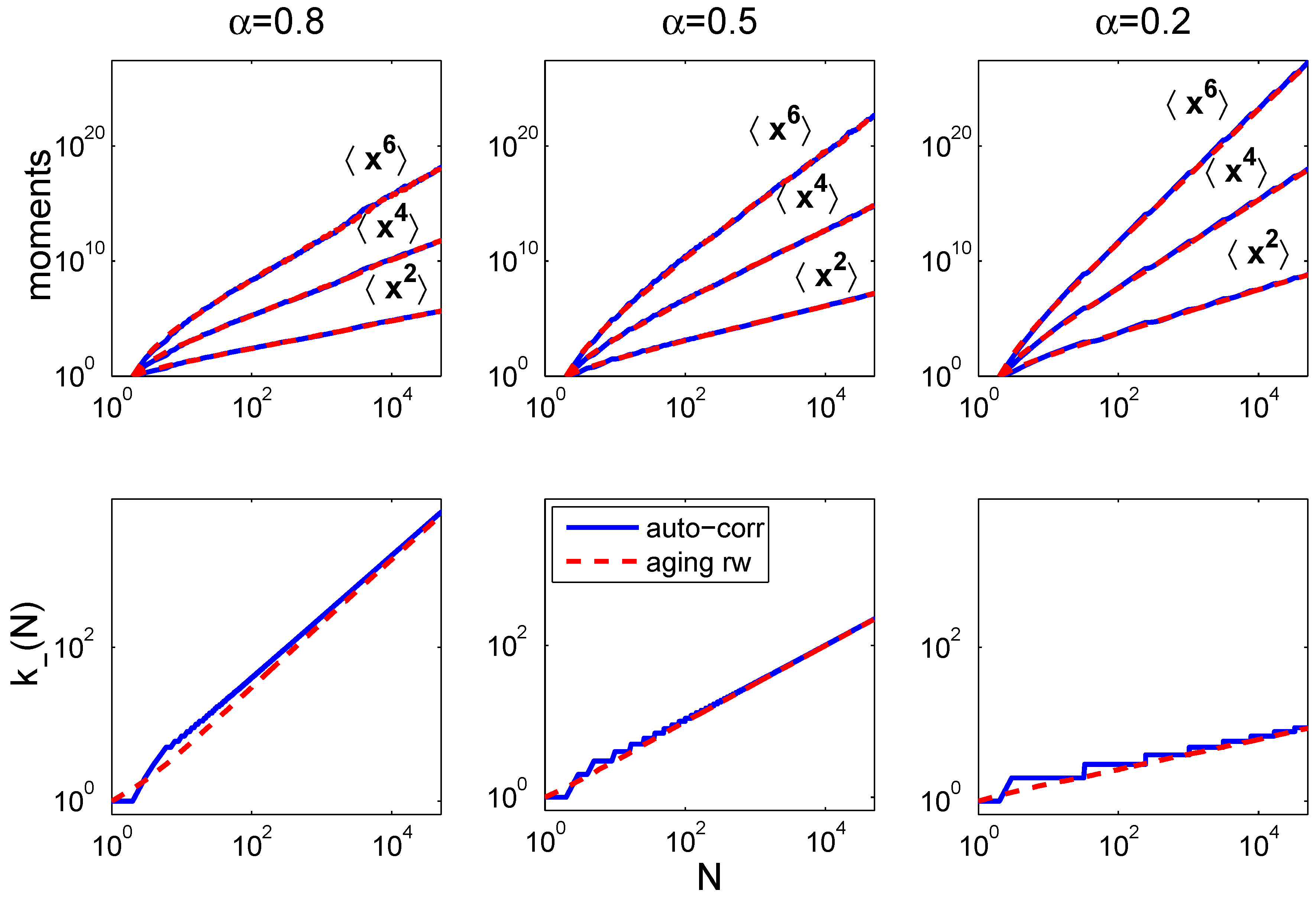
We demonstrated that the auto-correlated random walk characterized by $0<\alpha \le 1$ introduced in [2] cannot be distinguished from accelerating random walks in terms of distribution functions. Although the presented auto-correlated random walk is of entropy class $(c,d)=(1,1/\alpha )$, and the accelerated random walk is of class $(c,d)=(1,1)$, both processes have the same distribution function, since all moments, $\langle x^n\rangle$, are identical. We have shown that other classes of random walks can naturally be obtained, including those belonging to the $(c,d)=(q,0)$ (Tsallis) equivalence class. Moreover, we showed numerically that the auto-correlated random walk is asymptotically equivalent to a particular aging random walk, where the probability of a decision to reverse the direction of the walk depends on the path the random walk has taken. This concept of aging can easily be generalized to different forms of aging, and it can be expected that many of the admissible systems can be represented by a specific type of aging that is specified by the aging function, g. Finally, we have seen that different equivalence classes $(c,d)$ can be realized by specifying an aging function, g. The effective number of direction reversal decisions corresponding to the aging function remains finite, and therefore, the associated generalized entropy requires a class $(c,d)$ with $0<c<1$. We believe that it should be possible that the scheme of aging random walks can be naturally extended to aging processes in physical, biological and social systems.

References

1. Hanel, R.; Thurner, S. A comprehensive classification of complex statistical systems and an axiomatic derivation of their entropy and distribution functions. Europhys. Lett. 2011, 93, 20006. [Google Scholar] [CrossRef]
2. Hanel, R.; Thurner, S. When do generalized entropies apply? How phase space volume determines entropy. Europhys. Lett. 2011, 96, 50003. [Google Scholar] [CrossRef]
3. Thurner, S.; Hanel, R. What Do Generalized Entropies Look Like? An Axiomatic Approach for Complex, Non-Ergodic Systems. In Recent Advances in Generalized Information Measures and Statistics; Kowalski, A.M., Rossignoli, R., Curado, E.M.F., Eds.; Bentham Science eBook: Sharjah, United Arab Emirates, 2013; in press. [Google Scholar]
4. Shannon, C.E. A Mathematical theory of communication. Bell Syst. Tech. J. 1948, 27, 379–423, 623–656. [Google Scholar]
5. Khinchin, A.I. Mathematical Foundations of Information Theory; Dover Publications: Mineola, NY, USA, 1957. [Google Scholar]
6. Tsallis, C. Possible generalization of Boltzmann-Gibbs statistics. J. Stat. Phys. 1988, 52, 479–487. [Google Scholar] [CrossRef]
7. Anteneodo, C.; Plastino, A.R. Maximum entropy approach to stretched exponential probability distributions. J. Phys. A: Math Gen. 1999, 32, 1089–1097. [Google Scholar] [CrossRef]
8. Kaniadakis, G. Statistical mechanics in the context of special relativity. Phys. Rev. E 2002, 66, 056125. [Google Scholar] [CrossRef]
9. Curado, E.M.F.; Nobre, F.D. On the stability of analytic entropic forms. Phys. Stat. Mech. Appl. 2004, 335, 94–106. [Google Scholar] [CrossRef]
10. Tsekouras, G.A.; Tsallis, C. Generalized entropy arising from a distribution of q indices. Phys. Rev. E 2005, 71, 046144. [Google Scholar] [CrossRef]
11. Hanel, R.; Thurner, S. Generalized Boltzmann factors and the maximum entropy principle: Entropies for complex systems. Phys. Stat. Mech. Appl. 2007, 380, 109–114. [Google Scholar] [CrossRef]
12. Ubriaco, M.R. Entropies based on factional calculus. Phys. Lett. A 2009, 373, 2516–2519. [Google Scholar] [CrossRef]
13. Tsallis, C. Introduction to Nonextensive Statistical Mechanics; Springer: New York, NY, USA, 2009. [Google Scholar]
14. Shafee, F. Lambert function and a new non-extensive form of entropy. IMA J. Appl. Math. 2007, 72, 785–800. [Google Scholar] [CrossRef]
15. Hanel, R.; Thurner, S.; Gell-Mann, M. Generalized entropies and the transformation group of superstatistics. Proc. Natl. Acad. Sci. USA 2011, 108, 6390–6394. [Google Scholar] [CrossRef]
16. Hanel, R.; Thurner, S.; Gell-Mann, M. Generalized entropies and logarithms and their duality relations. Proc. Natl. Acad. Sci. USA 2012, 109, 19151–19154. [Google Scholar] [CrossRef] [PubMed]
17. Lesche, B. Instabilities of Rényi entropies. J. Stat. Phys. 1982, 27, 419–422. [Google Scholar] [CrossRef]
18. Abe, S. Stability of Tsallis entropy and instabilities of Rényi and normalized Tsallis entropies. Phys. Rev. E 2002, 66, 046134. [Google Scholar] [CrossRef]
19. Jizba, P.; Arimitsu, T. Observability of Rényis entropy. Phys. Rev. E 2004, 69, 026128. [Google Scholar] [CrossRef]
20. Kaniadakis, G.; Scarfone, A.M. Lesche stability of κ-entropy. Phys. Stat. Mech. Appl. 2004, 340, 102–109. [Google Scholar] [CrossRef]
21. Hanel, R.; Thurner, S.; Tsallis, C. On the robustness of q-expectation values and Rényi entropy. Europhys. Lett. 2009, 85, 20005. [Google Scholar] [CrossRef]
22. Tsallis, C.; Gell-Mann, M.; Sato, Y. Asymptotically scale-invariant occupancy of phase space makes the entropy Sq extensive. Proc. Natl. Acad. Sci. USA 2005, 102, 15377–15382. [Google Scholar] [CrossRef] [PubMed]