Dynamics of Instantaneous Condensation in the ZRP Conditioned on an Atypical Current

Abstract

Using a generalized Doob’s h-transform we consider the zero-range process (ZRP) conditioned to carry an atypical current, with focus on the regime where the Gallavotti-Cohen symmetry loses its validity. For a single site we compute explicitly the boundary injection and absorption rates of an effective process which maps to a biased random walk. Our approach provides a direct probabilistic confirmation of the theory of “instantaneous condensation” which was proposed some while ago to explain the dynamical origin of the the failure of the Gallavotti-Cohen symmetry for high currents in the ZRP. However, it turns out that for stochastic dynamics with infinite state space care needs to be taken in the application of the Doob’s transform—we discuss in detail the sense in which the effective dynamics can be interpreted as “typical” for different regimes of the current phase diagram.

1. Introduction

Non-equilibrium dynamics is rather generally governed by many so-called fluctuation relations, which can all be derived from a fundamental time-reversal property, as shown in [1] and recently further elaborated in [2]. In particular, the Gallavotti-Cohen Fluctuation Theorem relates the asymptotic probability of an entropy production to the probability of a negative entropy production of the same absolute value [3] and generically leads to a similar symmetry for currents in interacting particle systems [4]. Despite the very general validity of this Gallavotti-Cohen symmetry (GCS), subtle and often not well-understood effects can cause a breakdown. This was discussed in [5,6] for Langevin dynamics and in some detail in [7,8] in the context of current fluctuations in the zero-range process (ZRP) [9,10]. Specifically, in [7,8], a mechanism dubbed “instantaneous condensation” was proposed as the dynamical origin of the failure of the GCS at high currents. It was noted that unstable condensates (hence called “instantaneous”) can form due to fluctuations, and it was argued that if the dynamics enters a regime of atypically large current through a prolonged fluctuation, then the distribution of the current undergoes non-analytic changes. Indeed, an interesting current phase diagram with distinct regimes of current fluctuations was thus discovered.

Here we reconsider this scenario from a different angle which has become popular recently in the study of phase transitions induced by conditioning a particle system on atypical currents; see, e.g., [11,12,13,14,15,16,17]. In this approach one studies, through a generalized Doob’s h-transform [18,19], the external forces under which an atypical fluctuation becomes typical. This establishes an equivalence between (i) conditioning a given system on an atypical fluctuation and (ii) an effective dynamics with modified interactions in which the conditioned behaviour becomes typical. Thus, one gains direct insight into the dynamics that govern a system during a rare atypical fluctuation.

We shall demonstrate that the theory of “instantaneous condensation”, which was developed via a mathematical saddle-point analysis in [7,8] to explain the failure of the GCS is correct. Since this failure occurs already at the level of a single-site lattice, we focus here on this case and explicitly construct a corresponding Doob’s transform yielding effective dynamics, which is a biased random walk on the set of non-negative integers. Studying the exponential moments of the position of the random walk with a geometric initial distribution then not only reproduces the phase diagram found earlier, but also provides insight into the formation of instantaneous condensates. In the process, we highlight some subtleties involved in the application of Doob’s transform to systems with infinite state space and shed light on the conditions needed for the equivalence between (i) and (ii) above.

The paper is organized as follows. In Section 2, we informally describe the well-established, but not so widely known, tools required for studying grand-canonically conditioned dynamics. In Section 3, we perform the analysis of the current distribution in terms of the effective random walk dynamics, and in Section 4, we specifically consider the dynamics of instantaneous condensates. In Section 5, we conclude and discuss our findings in light of the results of [7,8].

2. The Zero Range Process and Grand Canonical Current Conditioning

The ZRP [9,10] describes the Markovian time evolution of identical particles on $\mathbb{Z}$ according to the following rules: (1) each particle jumps after an exponentially distributed random time with mean $n/w_n$ from a site with $n>0$ particles with probability $c_r$ to the right neighbouring site and $c_{\ell }$ to the left neighbouring site (zero-range interaction between particles); (2) the jumps occur independently of each other (Markov property). Without loss of generality, we shall assume $c_r>c_{\ell }$, which corresponds to a bias due to some external driving force. For a finite chain with L sites, these bulk rules have to be supplemented by boundary conditions. In the case of open boundary conditions, particles are injected onto Site 1 (L) with rate α (δ), and a particle is removed with rate $\gamma w_n$ ($\beta w_n$). One can think of these boundary processes as resulting from a left particle reservoir at a virtual Site 0 and a right particle reservoir at Site $L+1$.

A microstate of the system $\eta =\left\{\eta \right(1),\eta (2),\cdots ,\eta (L\left)\right\}$ is given by the non-negative integer occupation numbers $\eta \left(k\right)\in {\mathbb{N}}_0$ at sites $k\in \{1,2,\cdots ,L\}$. We define the kth bond of the lattice to be between sites k and $k+1$, including the virtual boundary sites. In a periodic chain an important family of invariant measures for this process are the Bernoulli product measures parametrised by the particle density ρ [9,10]. The stationary current expectation $j^{*}$ is then $j^{*}=(c_r-c_{\ell })z\left(\rho \right)$, where $z\left(\rho \right)$ is the fugacity thermodynamically conjugate to the density. For $c_r=c_{\ell }$ (symmetric ZRP), the dynamics is reversible, and one has $j^{*}=0$. In the open system the invariant measure (if it exists) is unique and given by a product measure with, in general, space-dependent local fugacities $z_k$ that depend on the boundary parameters $\alpha ,\beta ,\gamma ,\delta$ [20].

A convenient way to describe the stochastic time evolution is in terms of the quantum Hamiltonian formulation [21,22] of the master equation:

$$\frac{\mathrm{d}}{\mathrm{d}t}|P\left(t\right)\rangle =-H|P\left(t\right)\rangle$$

(1)

where the probability vector $|P\left(t\right)\rangle$ has as its components the time-dependent probabilities $P(\eta ,t)$ of finding the microstate η at time $t\ge 0$ and the generator H has as off-diagonal matrix elements the negative transition rates $w({\eta }^{\prime },\eta )$ for a transition from η to ${\eta }^{\prime }$ and on the diagonal the sum of outgoing rates ${\sum }_{\eta }w({\eta }^{\prime },\eta )$ from a microstate η. The solution of Equation (1) is given by

$$|P\left(t\right)\rangle ={\mathrm{e}}^{-Ht}|P\left(0\right)\rangle$$

(2)

for an initial distribution $|P\left(0\right)\rangle$. We shall denote an initial distribution concentrated on a single microstate by $|\eta \rangle$ and impose an orthogonality relation $\langle {\eta }^{\prime }|\eta \rangle ={\delta }_{{\eta }^{\prime },\eta }$ with the dual basis vectors $\langle \eta |$. By definition, the stationary probability vector, denoted $|P^{*}\rangle$, is a right eigenvector of H with an eigenvalue of zero. The left eigenvector of H with an eigenvalue of zero is the summation vector $\langle s|={\sum }_{\eta }\langle \eta |$ whose components are all equal to one, expressing conservation of probability $\langle s|P\left(t\right)\rangle =1$ $\forall t\ge 0$.

Expectation values of a function $f\left(\eta \right)$ are given by

$$\langle f\left(t\right)\rangle =\langle s|\widehat{f}|P\left(t\right)\rangle =\sum _{\eta }f\left(\eta \right)P(\eta ,t)$$

(3)

where the object $\widehat{f}$ is a diagonal matrix with elements $f\left(\eta \right)$ on the diagonal. Specifically, for a fixed initial state ${\eta }_1$ and $\widehat{f}=|{\eta }_2\rangle \langle {\eta }_2|$, we obtain the microscopic transition probability

$$P({\eta }_2,t|{\eta }_1,0)=\langle {\eta }_2|{\mathrm{e}}^{-Ht}|{\eta }_1\rangle .$$

(4)

An expectation value can also be expressed as the matrix element

$$\langle f\left(t\right)\rangle =\langle s|\widehat{f}\left(t\right)|P\left(0\right)\rangle$$

(5)

of the time-dependent operator

$$\widehat{f}\left(t\right)={\mathrm{e}}^{Ht}\widehat{f}{\mathrm{e}}^{-Ht}.$$

(6)

In this way, one can express multi-time expectations of observables $f_i$ at times $t_i$ as time-ordered matrix elements $\langle s|\widehat{f_n}\left(t_n\right)\cdots \widehat{f_1}\left(t_1\right)|P\left(0\right)\rangle$ with $t_i\ge t_{i-1}$.

Of particular interest in the study of the ZRP and other stochastic interacting particle systems, is the time-integrated current $J_k\left(t\right)=J_k^{+}\left(t\right)-J_k^{-}\left(t\right)$ across a bond $(k,k+1)$, where $J_k^{+}\left(t\right)$ is the number of jumps of particles from site k to $k+1$ up to time t, and analogously, $J_k^{-}\left(t\right)$ is the number of jumps from $k+1$ to k up to time t, starting from some initial distribution of the particles at time zero. A related quantity of interest is the time-integrated total current $J\left(t\right)={\sum }_k{J}_k\left(t\right)$, which is intimately related to the entropy production [1,4]. One also considers the (local) time-averaged current $j_k\left(t\right)=J_k\left(t\right)/t$ and the (global) time-averaged current density $j\left(t\right)=J\left(t\right)/\left(Lt\right)$. For the stationary distribution, one has, by the law of large numbers ${lim}_{t\to \infty }{j}_k\left(t\right)={lim}_{t\to \infty }j\left(t\right)=j^{*}$, where $j^{*}$ is the current expectation. The probability of observing for a long time interval t an atypical mean $j\ne j^{*}$ is exponentially small in t. This is expressed in the large deviation property [4,23] $\mathrm{Prob}\left[J\left(t\right)=J\right]\propto exp(-f(j\left)Lt\right)$, where $f\left(j\right)$ is the rate function, which plays a role analogous to the free energy in equilibrium statistical mechanics. Indeed, in complete analogy to equilibrium, one introduces a generalized chemical potential s and also studies the generating function $Y_s\left(t\right)=\langle {\mathrm{e}}^{sJ\left(t\right)}\rangle ={\sum }_J{\mathrm{e}}^{sJ}\mathrm{Prob}\left[J\left(t\right)=J\right]$ of the time-integrated current. The cumulant function $g\left(s\right)={lim}_{t\to \infty }ln{Y}_s\left(t\right)/\left(Lt\right)$ is the Legendre transform of the rate function for the time-averaged current, $g\left(s\right)={max}_j[js-f\left(j\right)]$. The intensive variable s is thus conjugate to the time-averaged current density j. The Gallavotti-Cohen symmetry (GCS) predicts [3,4]

$$f\left(j\right)-f(-j)=Fj$$

(7)

with a model-dependent constant F which in the context of particle systems, has a natural interpretation as a driving field [4,8].

As mentioned in the introduction, it was found in [7] that the GCS Equation (7) can fail in the ZRP for sufficiently atypical mean currents. This was demonstrated by direct solution of the master equation for a ZRP with a single site using a saddle-point approximation. In order to shed more light on this phenomenon, we choose here a different approach: We aim to study the dynamics conditioned on a prolonged atypical behaviour rather than analyzing rare fluctuations. A convenient way to do so is to consider the process in terms of the conjugate variable s. Fixing some $s\ne 0$ corresponds to studying atypical realizations of the process in which the current fluctuates around some non-typical mean. We shall refer to this approach as grand canonical conditioning, as opposed to a canonical condition in which the current would be conditioned to have some fixed value. We remark that the grand-canonically conditioned ensemble is sometimes called the s-ensemble, but we do not adopt this nomenclature here.

We outline the strategy of grand canonical conditioning in general terms, since it works in a similar way for any integrated current, in particular for the integrated bond currents $J_k\left(t\right)$, not just for the total current. Correspondingly, in the remainder of this section $Y_s\left(t\right)$ is a generic generating function for the current across some bond (which we do not specify here), $g\left(s\right)$ is the corresponding large deviation function (without a factor of L as above for the total current) and $j\left(s\right)$ is the current on which we condition as a function of the conjugate variable s.

The generator of the grand canonically conditioned dynamics $H\left(s\right)$ is obtained from H by multiplying each off-diagonal matrix element that corresponds to a positive (negative) increment of the current under consideration by ${\mathrm{e}}^s$ (${\mathrm{e}}^{-s}$) [1,23]. The conditioned probability distribution $P_s(\eta ,t)$ is given by the probability vector

$$|P_s\left(t\right)\rangle =\frac{{\mathrm{e}}^{-H\left(s\right)t}|P\left(0\right)\rangle }{Y_s\left(t\right)}$$

(8)

where the generating function $Y_s\left(t\right)=\langle s|{\mathrm{e}}^{-H\left(s\right)t}|P\left(0\right)\rangle$ acts as normalization. This is a non-trivial function of s and t since the matrix $H\left(s\right)$ does not conserve probability. (Grand canonically) conditioned expectations at time t are then computed as follows:

$${\langle f\left(t\right)\rangle }_s=\frac{\langle s|\widehat{f}{\mathrm{e}}^{-H\left(s\right)t}|P\left(0\right)\rangle }{\langle s|{\mathrm{e}}^{-H\left(s\right)t}|P\left(0\right)\rangle }.$$

(9)

For processes with finite state space, one can easily prove various intriguing properties of the conditioned dynamics. In particular, the large deviation property of the current $Y_s\left(t\right)\propto {\mathrm{e}}^{g\left(s\right)t}$ can be expressed through the lowest eigenvalue $E_0\left(s\right)$ of $H\left(s\right)$ by the simple relation

$$g\left(s\right)=-E_0\left(s\right),$$

(10)

and therefore one has

$$j\left(s\right)=-\frac{d}{ds}{E}_0\left(s\right).$$

(11)

In terms of s, the GCS Equation (7) then follows from the spectral relation

$$E_0\left(s\right)=E_0(F-s).$$

(12)

In order to study the dynamics that make an atypical current $j\left(s\right)$ typical, the established prescription is to introduce a generalized Doob’s h-transform [18,19]

$$\tilde{H}\left(s\right)=\Delta \left(s\right)H\left(s\right)\Delta {\left(s\right)}^{-1}-E_0\left(s\right)$$

(13)

where $\Delta \left(s\right)$ is the diagonal matrix, which has the components ${\Delta }_{\eta }\left(s\right)$ of the lowest left eigenvector of $H\left(s\right)$ on the diagonal. This construction is based on the observation that (by definition) ${\Delta }_{\eta }\left(s\right)$ is a harmonic function for the weighted generator $H\left(s\right)$. Thus, the summation vector $\langle s|$ is a left eigenvector of $\tilde{H}\left(s\right)$ with an eigenvalue of zero. According to Perron-Frobenius, all components of this eigenvector are strictly positive real numbers (up to an irrelevant normalization) and therefore the non-diagonal elements ${\tilde{H}}_{{\eta }^{\prime },\eta }\left(s\right)$ of $\tilde{H}\left(s\right)$ are transition rates of a transformed process, which we shall call “effective dynamics” or “effective process”. The h-transform provides a means to tilt the measure on path space, such that an atypical current value becomes typical. We denote by $P_s^{*}\left(\eta \right)$ the invariant measure of the effective process $\tilde{H}\left(s\right)$. It is easy to prove that $P_s^{*}\left(\eta \right)\propto {\Delta }_{\eta }\left(s\right){\overline{\Delta }}_{\eta }\left(s\right)$, where ${\overline{\Delta }}_{\eta }\left(s\right)$ are the components of the lowest right eigenvector $|\overline{\Delta }\left(s\right)\rangle$ of $H\left(s\right)$. Below, we shall drop the argument s of $\tilde{H}$, $E_0$ and Δ, if there is no danger of confusion.

Generally speaking, the desired property of the effective process is that by conditioning over a very large time interval the matrix $\tilde{H}\left(s\right)$ becomes the generator of a stochastic dynamics whose transition rates define the interactions for which the conditioned dynamics become typical, see [13,14,17] for applications to currents and also [24,25,26] for more general context. To prove this, for finite state space, we consider a large time interval $[0,T]$ and fix a time $t\in [0,T]$.We start the original process at some fixed microstate ${\eta }_1$ and take at time t the projector $\widehat{f}=|{\eta }_2\rangle \langle {\eta }_2|$ on a microstate ${\eta }_2$. Then the l.h.s. of Equation (9) is the conditioned transition probability $P_{s,T}({\eta }_2,t|{\eta }_1,0)=\langle s|{\mathrm{e}}^{-H\left(s\right)t^{\prime }}\widehat{f}{\mathrm{e}}^{-H\left(s\right)t}|P\left(0\right)\rangle /Y_s\left(T\right)$ from ${\eta }_1$ at time zero to ${\eta }_2$ at time t with $t^{\prime }=T-t$. Using Equation (13), one obtains for $T\to \infty$

$$\begin{array}{ccc}\hfill \underset{T\to \infty }{lim}{P}_{s,T}({\eta }_2,t|{\eta }_1,0)& =& \underset{T\to \infty }{lim}\frac{\langle s|{\Delta }^{-1}{\mathrm{e}}^{-\tilde{H}(T-t)}|{\eta }_2\rangle \langle {\eta }_2|{\mathrm{e}}^{-\tilde{H}t}\Delta |{\eta }_1\rangle }{\langle s|{\Delta }^{-1}{\mathrm{e}}^{-\tilde{H}T}\Delta |{\eta }_1\rangle }\hfill \\ & =& \frac{\langle s|{\Delta }^{-1}|P_s^{*}\rangle \langle s|{\eta }_2\rangle \langle {\eta }_2|{\mathrm{e}}^{-\tilde{H}t}\Delta |{\eta }_1\rangle }{\langle s|{\Delta }^{-1}|P_s^{*}\rangle \langle s|\Delta |{\eta }_1\rangle }\hfill \\ & =& \langle {\eta }_2|{\mathrm{e}}^{-\tilde{H}t}|{\eta }_1\rangle =P_s({\eta }_2,t|{\eta }_1,0)\hfill \end{array}$$

(14)

The last line holds since $\langle s|{\eta }_i\rangle =1$ and $\Delta |{\eta }_1\rangle ={\Delta }_{{\eta }_1}|{\eta }_1\rangle$. Hence, in the large time limit $T\to \infty$, the conditioned transition probability of the original process is the (conventional) transition probability $P_s({\eta }_2,t|{\eta }_1,0)$ of the transformed effective process. Thus it becomes clear that $\tilde{H}$ generates a process in which the originally atypical current becomes typical.

For general initial distributions $P_0$ and observables f one obtains

$$\begin{array}{ccc}\hfill \underset{T\to \infty }{lim}{\langle f\left(t\right)\rangle }_{s,T}& =& \underset{T\to \infty }{lim}\frac{\langle s|{\Delta }^{-1}{\mathrm{e}}^{-\tilde{H}(T-t)}f{\mathrm{e}}^{-\tilde{H}t}\Delta |P_0\rangle }{\langle s|{\Delta }^{-1}{\mathrm{e}}^{-\tilde{H}T}\Delta |P_0\rangle }\hfill \\ & =& \frac{\langle s|f{\mathrm{e}}^{-\tilde{H}t}\Delta |P_0\rangle }{\langle s|\Delta |P_0\rangle }\hfill \\ & =& \langle s|f{\mathrm{e}}^{-\tilde{H}t}|{\tilde{P}}_0\rangle \hfill \end{array}$$

(15)

which is an expectation of the effective dynamics for a modified initial distribution ${\tilde{P}}_0\left(\eta \right)=\Delta \left(\eta \right)P_0\left(\eta \right)/{\langle \Delta \rangle }_{P_0}$.

On the other hand, for $T=t$ finite, the conditional expectation Equation (9) reads in terms of the effective process

$$\begin{array}{ccc}\hfill {\langle f\left(t\right)\rangle }_{s,t}& =& \frac{\langle s|f{\mathrm{e}}^{-H\left(s\right)t}|P_0\rangle }{\langle s|{\mathrm{e}}^{-H\left(s\right)t}|P_0\rangle }\hfill \\ & =& \frac{\langle s|f{\Delta }^{-1}{\mathrm{e}}^{-\tilde{H}t}\Delta |P_0\rangle }{\langle s|{\Delta }^{-1}{\mathrm{e}}^{-\tilde{H}t}\Delta |P_0\rangle }\hfill \\ & =& \frac{{\langle f\left(t\right){\Delta }^{-1}\left(t\right)\rangle }_{s,{\tilde{P}}_0}}{{\langle {\Delta }^{-1}\left(t\right)\rangle }_{s,{\tilde{P}}_0}}.\hfill \end{array}$$

(16)

It is also instructive to split $0,T$ into three subintervals $[0,{\tau }_1]$, $[{\tau }_1,{\tau }_2]$ and $[{\tau }_2,T]$. We fix $t\in [{\tau }_1,{\tau }_2]$ and first send both ${\tau }_1$ and $T-{\tau }_2$ to infinity, such that $[{\tau }_1,{\tau }_2]$ remains finite. Then

$$\underset{{\tau }_1\to \infty }{lim}\underset{T-{\tau }_2\to \infty }{lim}{\langle f\left(t\right)\rangle }_s=\langle s|f|P_s^{*}\rangle \forall t\in [{\tau }_1,{\tau }_2].$$

(17)

Analogously one can prove for $t_1,t_2\in [{\tau }_1,{\tau }_2]$ and $t_2\ge t_1$

$$\underset{{\tau }_1\to \infty }{lim}\underset{T-{\tau }_2\to \infty }{lim}{\langle f_2\left(t_2\right)f_1\left(t_1\right)\rangle }_s=\langle s|f_2{\mathrm{e}}^{-\tilde{H}(t_2-t_1)}{f}_1|P_s^{*}\rangle \forall t_1,t_2\in [{\tau }_1,{\tau }_2],$$

(18)

and similarly for multiple conditioned joint expectations. Hence, for infinite initial and terminal time intervals, the conditioned joint expectations of the original process turn into (usual) stationary joint expectations of the effective process.

Notice that, throughout the above discussion, finite state space is implicitly assumed so that relation Equation (10) is guaranteed to hold and the large deviation function $g\left(s\right)$ does not depend on the initial distribution of the process. The point of our analysis below is to investigate scenarios in the ZRP in which these conditions do not, in general, hold. It will transpire here that the “effective” dynamics is not always equivalent to the conditioned dynamics in the sense that the transformed process does not always represent the typical behaviour of the original process under conditioning.

3. Current Phase Diagram of the Single-Site Effective Dynamics

From now on, we consider the ZRP with $L=1$ which has an infinite state space. Each microstate η corresponds to a lattice site with $n=\eta$ particles. The corresponding basis vectors are denoted by $|n\rangle$ with integer argument n. We study the effective process and the long-time behaviour of current fluctuations at the entrance bond of zero between the left reservoir and site 1. Correspondingly, from now on the variable s is conjugate to the integrated current across this bond, and g(s) is the associated large deviation function. We take the initial distribution $P_0\left(n\right)=(1-x)x^n{\prod }_{i=1}^n{w}_i^{-1}$, denoted as $|x\rangle$. In general, x is a non-stationary initial fugacity (a natural way to think of this setting is that one lets the ZRP relax to a stationary distribution given by $|x\rangle$ and then, at time $t=0$, changes the boundary parameters, such that $|x\rangle$ is no longer stationary. Then, for $t>0$, one studies the conditioned dynamics for t large. Note that in order to ensure the ergodicity of the unconditioned dynamics, we require

$$\alpha +\delta <\beta +\gamma .$$

(19)

Except for extreme values of s, to be discussed below, $H\left(s\right)$ has a gapped spectrum with the lowest eigenvalue [7]

$$E_0\left(s\right)=({\mathrm{e}}^{-s}-1)\frac{\alpha \beta {\mathrm{e}}^s-\gamma \delta }{\beta +\gamma }$$

(20)

which satisfies the GCS Equation (7) with

$${\mathrm{e}}^F=\frac{\gamma \delta }{\alpha \beta }.$$

(21)

The corresponding lowest weighted left eigenvector has components

$${\Delta }_n=v^n$$

(22)

with

$$v=\frac{\beta +\gamma {\mathrm{e}}^{-s}}{\beta +\gamma }.$$

(23)

We use this eigenvalue and eigenvector to construct an effective process $\tilde{H}\left(s\right)$ according to the prescription Equation (13).

Some subtleties may be anticipated here, since, in contrast to the discussion of Section 2, we deal with an infinite state space (in particular, it is known that for certain choices of $w_n$ the spectrum becomes gapless for large magnitude s and the lowest eigenvalue crosses over to a different functional form). We stress that a Doob’s transform defined with $E_0\left(s\right)$ of Equation (20) and $\Delta \left(s\right)$ of Equation (22) can always be made, but the question of whether the resulting effective dynamics represents the original conditioned dynamics is non-trivial. Indeed, in the following, we show that the equivalence is a delicate issue, even in regimes in which the spectrum of $H\left(s\right)$ does have a gap.

The transformation matrix can be written $\Delta =v^{\widehat{N}}$ where $\widehat{N}={\sum }_{n=0}^{\infty }n|n\rangle \langle n|$ is the particle number operator. Note that the injection rates are multiplied by a factor v under this transformation and the extraction rates by $v^{-1}$. Therefore the effective dynamics is a ZRP, where injection (extraction) at the left boundary is given by the rate $\alpha v{\mathrm{e}}^s$ $\left(\gamma v^{-1}{\mathrm{e}}^{-s}{w}_n\right)$. At the right boundary, we have rates $\delta v$ for injection and $\beta v^{-1}{w}_n$ for extraction.

The lowest right eigenvector of $H\left(s\right)$ has components

$${\overline{\Delta }}_n=u^n\prod _{i=1}^n{w}_i^{-1}$$

(24)

where

$$u=\frac{\alpha {\mathrm{e}}^s+\delta }{\beta +\gamma }.$$

(25)

Defining $z=uv$ the stationary distribution of the effective dynamics is then given by

$$P_s^{*}\left(n\right)=\frac{1}{Z}{z}^n\prod _{i=1}^n{w}_i^{-1}$$

(26)

where

$$Z=\sum _{n=0}^{\infty }{z}^n\prod _{i=1}^n{w}_i^{-1}$$

(27)

is the local analogue of the grand-canonical partition function. We conclude that a stationary distribution exists only for a finite radius of convergence $z^{*}$ determined by the asymptotic behaviour of the product over the rates $w_i$. The corresponding effective stationary current as a function of s is

$$j^{*}\left(s\right)=\frac{\alpha \beta {\mathrm{e}}^s-\gamma \delta {\mathrm{e}}^{-s}}{\beta +\gamma }=-\frac{d}{ds}{E}_0\left(s\right).$$

(28)

Notice that this stationary current is the same as the conditioned current $j\left(s\right)$, defined as the derivative of the large deviation function $g\left(s\right)$, only when the transformed dynamics is equivalent to the conditioned dynamics, as discussed below.

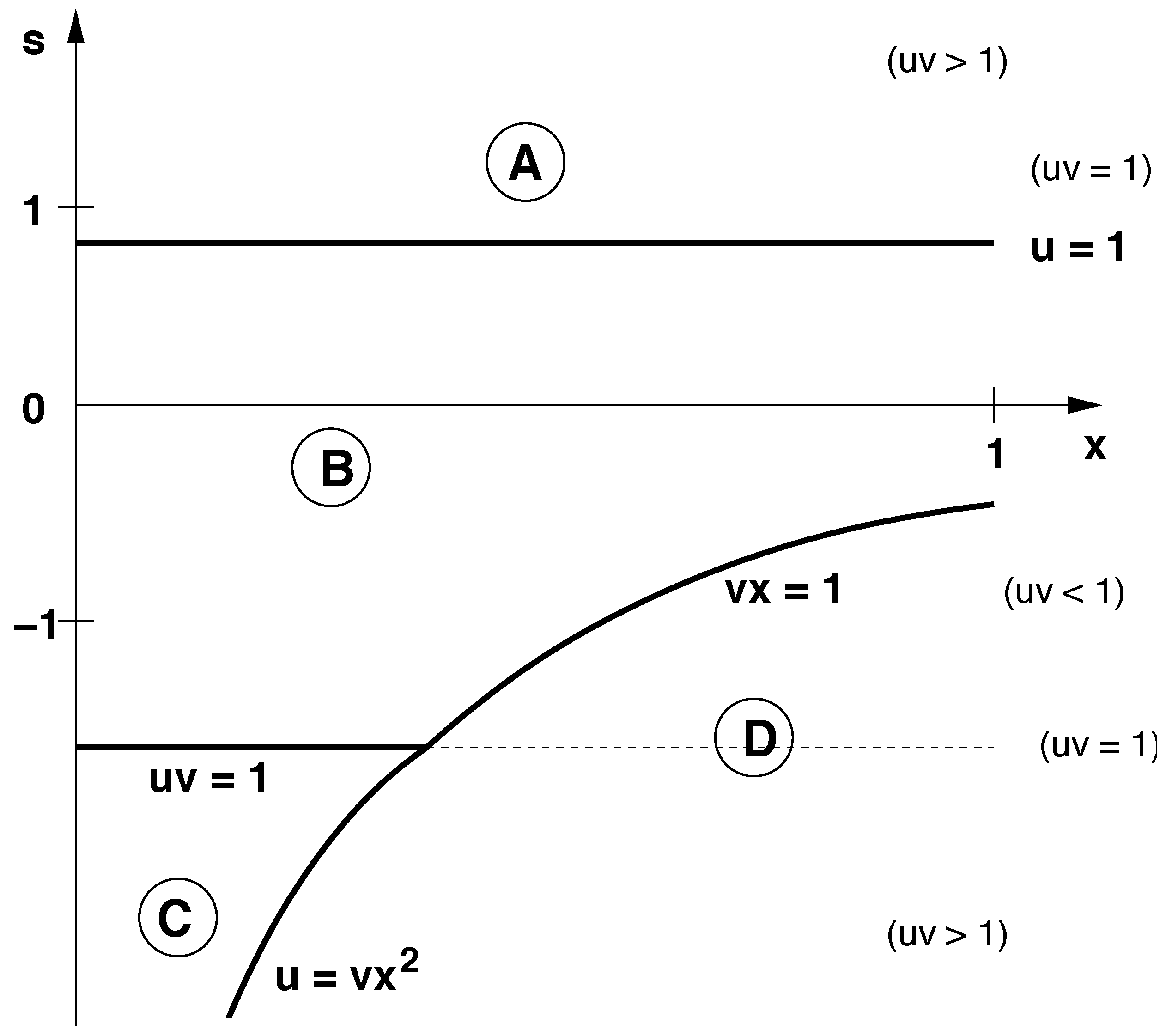
We focus now on the choice $w_n=1$, which implies a radius of convergence $z^{*}=1$. In this case, it was found in [7,8] that in terms of the conjugate variable s, there are four regimes with different distributions of the current and non-analytic changes along the transition lines— the phase diagram has the generic form shown in Figure 1. (One expects related phase diagrams for general hopping rates $w_n$ of the ZRP, with the location of the phase transition lines depending on the parameters.) In [7,8], the phase diagram was obtained through a saddle-point analysis of the normalization factor $Y_s\left(t\right)$. In this section, we consider the same problem from a more probabilistic perspective by analyzing in detail the properties of the transformed process. We thus not only recover the phase diagram, but also elucidate the validity of the equivalence between h-transformed and original conditioned dynamics and obtain more detailed insight into the formation of instantaneous condensates; see also the following section.

Figure 1. Generic phase diagram of the current distribution in terms of the conjugate parameter s and the initial distribution parameter x. The thick lines are phase transition lines between the phases A,B,C,D. The broken lines indicate the range of ergodicity $uv<1$ of the transformed dynamics.

Figure 1. Generic phase diagram of the current distribution in terms of the conjugate parameter s and the initial distribution parameter x. The thick lines are phase transition lines between the phases A,B,C,D. The broken lines indicate the range of ergodicity $uv<1$ of the transformed dynamics.

For the choice $w_n=1$, the effective dynamics of the single-site ZRP maps to a biased random walk on the non-negative integers ${\mathbb{N}}_0$ with hopping rate $p=uv(\beta +\gamma )$ to the right and hopping rate $q=\beta +\gamma$ to the left, identifying the occupation number n of the ZRP with the position of the random walker. The boundary at the origin is reflecting, i.e., jump attempts from zero to the left are rejected. By definition, the transition probability $C_{m,n}^{+}\left(t\right)=\langle m|{\mathrm{e}}^{-\tilde{H}t}|n\rangle$ of this random walk, with initial point n at time zero and end point m at time t, satisfies the master equation

$$\begin{array}{ccc}\hfill \frac{\mathrm{d}}{\mathrm{d}t}{C}_{m,n}^{+}\left(t\right)& =& p{C}_{m-1,n}^{+}\left(t\right)+q{C}_{m+1,n}^{+}\left(t\right)-(p+q)C_{m,n}^{+}\left(t\right)\mathrm{for} m>0\hfill \end{array}$$

(29)

$$\begin{array}{ccc}\hfill \frac{\mathrm{d}}{\mathrm{d}t}{C}_{0,n}^{+}\left(t\right)& =& q{C}_{1,n}^{+}\left(t\right)-p{C}_{0,n}^{+}\left(t\right)\hfill \end{array}$$

(30)

where $m,n\in {\mathbb{N}}_0$ with initial condition $C_{m,n}^{+}\left(0\right)={\delta }_{m,n}$. It is straightforward to verify that the solution for this problem is

$$\begin{array}{ccc}\hfill C_{m,n}^{+}\left(t\right)& =& {\mathrm{e}}^{-(p+q)t}{\left(\frac{p}{q}\right)}^{\frac{m-n}{2}}\left[I_{m-n}\left(2\sqrt{pq}t\right)+\sqrt{\frac{q}{p}}{I}_{m+n+1}\left(2\sqrt{pq}t\right)+\right.\hfill \\ \mathrm{(31)}& & & \left.\left(1-\frac{p}{q}\right)\sum _{k=2}^{\infty }{\left(\frac{q}{p}\right)}^{\frac{k}{2}}{I}_{m+n+k}\left(2\sqrt{pq}t\right)\right].\hfill \end{array}$$

To prove this one uses the relation $\mathrm{d}/\left(\mathrm{d}z\right)I_n\left(2z\right)=I_{n+1}\left(2z\right)+I_{n-1}\left(2z\right)$ of the modified Bessel function

$$I_n\left(2z\right)=\frac{1}{2\pi }{\int }_{-\pi }^{\pi }\mathrm{d}x{\mathrm{e}}^{ixn+2zcosx}.$$

(32)

In terms of the functions $u,v$ we may write

$$\begin{array}{ccc}\hfill C_{m,n}^{+}\left(t\right)& =& {\mathrm{e}}^{-E_{1}t}{\left(\sqrt{uv}\right)}^{m-n}[I_{m-n}\left(2E_{2}t\right)-(1-uv)I_{m+n}\left(2E_{2}t\right)\hfill \\ & & \left.+\sqrt{uv}{I}_{m+n+1}\left(2E_{2}t\right)+\left(1-uv\right)\sum _{k=0}^{\infty }{\left(\sqrt{uv}\right)}^{-k}{I}_{m+n+k}\left(2E_{2}t\right)\right]\hfill \\ & =:& {\mathrm{e}}^{-E_{1}t}{D}_{m,n}^{+}\left(t\right)\hfill \end{array}$$

(33)

with

$$E_1=p+q=(\beta +\gamma )(1+uv),E_2=\sqrt{pq}=(\beta +\gamma )\sqrt{uv}.$$

(34)

Here the function $D_{m,n}^{+}\left(t\right)$ has been introduced for convenience; see below. The random walk is ergodic for $p<q$ and relaxes to a geometric equilibrium distribution with parameter $p/q=uv<1$.

In random walk language, the quantities of interest for the calculation of the normalization factor $Y_s\left(t\right)$ (and hence extraction of the large deviation function) are the exponential moments $\langle v^{-m}\rangle$ of the particle position m at time t. This follows since

$$\begin{array}{ccc}\hfill Y_s\left(t\right)& =& \langle s|{\mathrm{e}}^{-H\left(s\right)t}|x\rangle \hfill \\ & =& {\mathrm{e}}^{-E_0\left(s\right)t}\langle s|{\Delta }^{-1}{\mathrm{e}}^{-\tilde{H}t}\Delta |x\rangle \hfill \\ & =& \frac{1-x}{1-vx}{\mathrm{e}}^{-E_0\left(s\right)t}\langle s|{\Delta }^{-1}{\mathrm{e}}^{-\tilde{H}t}|vx\rangle \hfill \end{array}$$

(35)

where the transformed initial condition is a geometric distribution with parameter $vx$. Hence, we can write

$$Y_s\left(t\right)=(1-x){\mathrm{e}}^{-(E_0+E_1)t}\sum _{m=0}^{\infty }\sum _{n=0}^{\infty }{v}^{n-m}{x}^n{D}_{m,n}^{+}\left(t\right).$$

(36)

Anticipating an exponential growth ${\mathrm{e}}^{Et}$ of the double sum yields the large deviation function

$$g\left(s\right)=-E_0\left(s\right)+E\left(s\right)-E_1\left(s\right).$$

(37)

We remark that power law prefactors that may arise in the double summation over $D_{m,n}^{+}\left(t\right)$ contribute only negligible corrections of order $ln\left(t\right)/t$ to $g\left(s\right)$.

For the subsequent analysis, we first list some exact formulae for sums of modified Bessel functions. By a shift of the integration variable $x\to x+i/2ln(p/q)$ in the complex plane one obtains the useful sum rule

$$\sum _{m=-\infty }^{\infty }{a}^m{I}_m\left(2zt\right)={\mathrm{e}}^{(a+a^{-1})zt}\forall a\in \mathbb{R}.$$

(38)

The following expressions for multiple sums for arbitrary arguments of the modified Bessel function can be obtained straightforwardly by shifting and reordering of the summation indices. First, one has

$$\sum _{m=0}^{\infty }\sum _{n=0}^{\infty }{a}^m{b}^n{I}_{n-m}=\frac{1}{1-ab}\sum _{n=0}^{\infty }(a^n+b^n)I_n-\sum _{n=0}^{\infty }{\left(ab\right)}^n{I}_n\left|ab\right|<1.$$

(39)

It turns out that the range $ab\ge 1$ is not required here, since in the double sum occurring in Equation (36), which involves $I_{n-m}$, we have

$$a=\sqrt{\frac{u}{v}},b=x\sqrt{\frac{v}{u}}$$

(40)

from which it follows that $ab=x<1$.

Moreover, for $a\ne b$ one has

$$\sum _{m=0}^{\infty }\sum _{n=0}^{\infty }{a}^m{b}^n{I}_{n+m+r}=\frac{a}{a-b}\sum _{n=0}^{\infty }{a}^n{I}_{n+r}+\frac{b}{b-a}\sum _{n=0}^{\infty }{b}^n{I}_{n+r}\forall r\in \mathbb{Z}.$$

(41)

For the triple sum we have

$$\begin{array}{ccc}\hfill \sum _{m=0}^{\infty }\sum _{n=0}^{\infty }\sum _{k=0}^{\infty }{a}^m{b}^n{c}^k{I}_{n+m+k}& =& \frac{a^2}{(a-b)(a-c)}\sum _{n=0}^{\infty }{a}^n{I}_n\hfill \\ & & +\frac{b^2}{(b-a)(b-c)}\sum _{n=0}^{\infty }{b}^n{I}_n\hfill \\ & & +\frac{c^2}{(c-b)(c-a)}\sum _{n=0}^{\infty }{c}^n{I}_n\hfill \end{array}$$

(42)

provided that all parameters $a,b,c$ are different from each other. In the triple sum occurring in Equation (36), we have

$$a=\sqrt{\frac{u}{v}},b=x\sqrt{\frac{v}{u}},c=\frac{1}{\sqrt{uv}}.$$

(43)

Similar expressions can be obtained when two or three parameters are equal, but these expressions turn out to be irrelevant here, since they change only prefactors that are algebraic in time and, hence, give only vanishing contributions to $g\left(s\right)$.

As a final preparatory step, we list well-known asymptotic properties of the modified Bessel function. For large z and $n\propto \sqrt{z}$ one has

$$I_n\left(2zt\right)=\frac{1}{\sqrt{4\pi zt}}{\mathrm{e}}^{-n^2/\left(4zt\right)}.$$

(44)

In particular, for n fixed and finite this yields $I_n\left(2zt\right)=\frac{1}{\sqrt{4\pi zt}}$ up to corrections of order $n^2/\left(zt\right)$. Equation (38) yields the following leading order asymptotics for the half-infinite sums

$$\sum _{m=0}^{\infty }{a}^m{I}_{m+r}\left(2zt\right)=\left\{\begin{array}{cc}\frac{1}{1-a}\frac{{\mathrm{e}}^{2zt}}{\sqrt{4\pi zt}}\hfill & \left|a\right|<1\hfill \\ & \\ \frac{1}{2}{\mathrm{e}}^{2zt}\hfill & a=1\hfill \\ & \\ a^{-r}{\mathrm{e}}^{(a+a^{-1})zt}\hfill & \left|a\right|>1.\hfill \end{array}\right.$$

(45)

Here r is fixed and finite, i.e., does not scale with z.

We are now in a position to determine the asymptotic properties of $Y_s\left(t\right)$ as a function of s and the initial value parameter x by extracting the leading order term in the sum Equation (36) over $D_{m,n}^{+}$.

For a given set of parameters $\alpha ,\beta ,\gamma ,\delta$ the asymptotics are encoded in $u\left(s\right)$ and $v\left(s\right)$. There are various regimes to consider.

(A) We observe that $u\ge 1$ implies $s>0$ (because of the ergodicity condition Equation (19)) which in turn implies $v<1$. Therefore in the range $u\ge 1$ one has $u>v$. Comparing the contributions in this range from the various sum Equations (39)–(42) applied to $D_{m,n}^{+}$ one finds that, independently of x and v, the leading contribution comes from the summation involving $a>1$. Then Equation (45) yields $D_{m,n}^{+}\left(t\right)\propto {\mathrm{e}}^{(a+a^{-1})E_{2}t}$. Thus Equation (37) together with Equation (34) leads to $E\left(s\right)=(\beta +\gamma )(u+v)$, and with Equation (20) we arrive at

$$g_A\left(s\right)=\alpha ({\mathrm{e}}^s-1)+\gamma ({\mathrm{e}}^{-s}-1)\ne -E_0\left(s\right).$$

(46)

Notice that the product $uv=p/q$ can be larger or smaller than 1one for $u\ge 1$. Hence in regime A it is not relevant for the large deviation function whether the random walk is ergodic ($uv<1$) or not $(uv\ge 1)$. This may appear surprising at first sight since in the transient case most of the weight is in configurations with large final positions of the random walk, which are highly unlikely (have exponentially small probability) in the ergodic case. However, although the decay of the ergodic stationary distribution is geometric with parameter $z=uv$, the exponential moment with parameter $1/v$ diverges for $u>1$, so, also, in this ergodic case, a lot of weight is given to random realizations of the biased random walk that ended up at large positions m.

This analysis is confirmed mathematically by approximating the transition probability $C_{m,n}^{+}\left(t\right)$ by its counterpart in an infinite lattice which is

$$\begin{array}{ccc}\hfill C_{m,n}\left(t\right)& =& {\left(\frac{p}{q}\right)}^{\frac{m-n}{2}}{\mathrm{e}}^{-(p+q)t}{I}_{m-n}\left(2\sqrt{pq}t\right)\hfill \\ \mathrm{(47)}& & =& {\mathrm{e}}^{-(p+q)t}\frac{1}{2\pi }{\int }_{-\pi }^{\pi }\mathrm{d}x{\mathrm{e}}^{ix(m-n)+(p{\mathrm{e}}^{-ix}+q{\mathrm{e}}^{ix})t}.\hfill \end{array}$$

The second line can be obtained from Equation (32) by a shift of the integration variable $x\to x+i/2ln(p/q)$ in the complex plane. Furthermore, since the contribution to $Y_s\left(t\right)$ is small for small final positions m, we can extend the summation over all final positions $m\in \mathbb{Z}$. This yields, indeed, Equation (46).

We note that the large weight attached to exponentially unlikely trajectories in the effective process indicates that the transformed dynamics in this regime does not represent the typical behaviour of the conditioned process. Technically, the effective dynamics is not equivalent to the conditioned dynamics since the quantity $\langle s|{\Delta }^{-1}|P_s^{*}\rangle$ in Equation (14) diverges. Nevertheless, as hinted at here and explored further in the next section, the transformed dynamics still provides useful information about the conditioned dynamics.

The remaining regimes all have $u<1$. First, we focus on small x.

(B) In addition to $u<1$ we consider the range $uv<1$ which is the ergodic regime $p/q=uv<1$ of the random walk and take $vx<1$. By inspection of the leading terms in the sums applied to $D_{m,n}^{+}$, one finds that in this range, the leading contribution comes from the summation involving $c=1/\sqrt{uv}>1$. Then Equation (37) together with Equation (45) yields $E\left(s\right)=(1/\sqrt{uv}+\sqrt{uv})(\beta +\gamma )\sqrt{uv}=(\beta +\gamma )(1+uv)=E_1\left(s\right)$. Therefore

$$g_B\left(s\right)=-E_0\left(s\right).$$

(48)

This result can be understood more directly in terms of the ergodicity of the random walk. For any finite initial position, it relaxes to a geometric equilibrium distribution with parameter $p/q=uv<1$. In this case ${lim}_{t\to \infty }{C}_{m,n}^{+}\left(t\right)=(1-uv){\left(uv\right)}^m$ and we obtain Equation (48) directly by noting that, for small x, the weight of large initial positions is small and, hence, does not contribute significantly to the double summation over $C_{m,n}^{+}\left(t\right)$. In this regime the effective dynamics is still equivalent to the conditioned dynamics, despite the infinite state space.

(C) We stay with small x and consider $u<1$ and $uv>1$ which is the transient regime of the random walk. In this case also $u<v$ and all three parameters $a,b,c$ are less than one, provided that $x<\sqrt{u/v}$. Hence, with the definition Equation (37) one has $E\left(s\right)=2E_2\left(s\right)=2\sqrt{uv}(\beta +\gamma )$. This yields

$$g_C\left(s\right)=2(\beta +\gamma )\sqrt{uv}-(\alpha +\beta +\gamma +\delta )\ne -E_0\left(s\right).$$

(49)

This result can also be directly derived by looking at the properties of the random walk. It is driven away from the origin and has a diffusive peak around its mean position $\overline{x}\left(t\right)=(p-q)t\gg 0$ for large t. Hence, we can approximate the transition probability $C_{m,n}^{+}\left(t\right)$ by its value Equation (47) in an infinite lattice, which is the first term in the sum Equation (31). In this case of small x the weight of large initial values of the random walk position is not strong enough to have an effect on the asymptotics of $Y_s\left(t\right)$. The expected exponential moment mainly picks up contributions from small final positions m. Hence the exponential growth of $D_{m,n}^{+}$ is dominated by the exponential factor ${\mathrm{e}}^{2\sqrt{uv}(\beta +\gamma )t}$ which together with the prefactor ${\mathrm{e}}^{-(\beta +\gamma )(1+uv)t}$ leads more directly to Equation (49).

Here again, the transformed dynamics does not represent typical behaviour of the conditioned process. In this case, the reason for the failure of the equivalence analysis in Equation (14) is that the spectrum of $H\left(s\right)$ becomes gapless. In fact, the lowest eigenvalue of this gapless spectrum is $-g_C\left(s\right)$.

For sufficiently large x, the situation is more complex, since large initial positions play a role in the double sum. First we consider the ergodic case $uv<1$.

(D1) For $u<1$, $uv<1$ and $vx>1$ the leading term in the sums applied to $D_{m,n}^{+}$ comes from $b=x\sqrt{(v/u)}>1$. Hence from Equation (37), it follows that $E\left(s\right)=(\beta +\gamma )(x\sqrt{(v/u)}+x^{-1}\sqrt{(u/v)})\sqrt{uv}=(\beta +\gamma )(xv+x^{-1}u)$. This yields

$$g_{D1}\left(s\right)=(\beta +\gamma {\mathrm{e}}^{-s})x+(\alpha {\mathrm{e}}^s+\delta )/x-(\alpha +\beta +\gamma +\delta )\ne -E_0\left(s\right).$$

(50)

In this case, a lot of weight is given to random realizations of the biased random walk, which started at large position n. Indeed, by time reversal we obtain $\langle s|{\Delta }^{-1}{\mathrm{e}}^{-\tilde{H}t}|y\rangle =(1-y)\langle s|X{\overline{\Delta }}^{-1}{\mathrm{e}}^{-\tilde{H}t}\overline{\Delta }|s\rangle =(1-y)/(1-y^{\prime })\langle s|{{\Delta }^{\prime }}^{-1}{\mathrm{e}}^{-\tilde{H}t}|y^{\prime }\rangle$, where ${\Delta }^{\prime }$ is similar to Δ but with v replaced by $u/x$, $y^{\prime }=u$ and X is the diagonal operator with $x^m$ on the diagonal. An analysis similar to Case B then also yields Equation (50).

(D2) For $u<1$, $uv>1$ and $x>\sqrt{u/v}$, the leading term in the sums applied to $D_{m,n}^{+}$ comes from $b=x\sqrt{(v/u)}>1$ as in Range (D1). Hence also here one has

$$g_{D2}\left(s\right)=(\beta +\gamma {\mathrm{e}}^{-s})x+(\alpha {\mathrm{e}}^s+\delta )/x-(\alpha +\beta +\gamma +\delta )=g_{D1}\left(s\right)\ne -E_0\left(s\right).$$

(51)

Since the behaviour of the large deviation function is identical in D1 and D2, we call the union of both domains D and define $g_D\left(s\right):=g_{D1}\left(s\right)=g_{D2}\left(s\right)$. In this regime, the transformed dynamics does not represent the typical behaviour of the conditioned process, because the matrix element $\langle s|\Delta |P_0\rangle$ in Equation (15) diverges, i.e., the modified initial distribution cannot be normalized. This is reflected in the dependence of the current large deviation function on the initial condition (via the fugacity x), even though we work in the limit of large t.

Finally, we discuss the critical line $uv=1$. Here the random walk is symmetric and its mean position diverges diffusively rather than ballistically. The transition probability reduces to

$$C_{m,n}^{+}\left(t\right)={\mathrm{e}}^{-(\beta +\gamma )t}\left[I_{m-n}\left(2(\beta +\gamma )t\right)+I_{m+n+1}\left(2(\beta +\gamma )t\right)\right].$$

(52)

For $x>1/v$ the analysis is similar to Case D. On the other hand, for $x<1/v$ one finds that, on the line $uv=1$, the functions $g_C\left(s\right)$ and $-E_0\left(s\right)$, coincide, and therefore, it is concluded that $Y_s\left(t\right)\propto {\mathrm{e}}^{-E_0\left(s\right)t}$. At $x=1/v$, one has $\Delta |x\rangle =|s\rangle$, where each component in $|s\rangle$ is 1. This vector is stationary w.r.t. $\tilde{H}$and therefore $Y_s\left(t\right)={\mathrm{e}}^{-E_0\left(s\right)t}$.

To summarize, there are four different regimes for the large deviation function, which is continuous, but non-analytic at the critical lines. Remarkably the ergodicity of the random walk is of limited significance for the form of the large deviation function. Only in Region B is the current distribution characterized by $g\left(s\right)=-E_0\left(s\right)$ where $E_0\left(s\right)$ is the lowest eigenvalue of $H\left(s\right)$ with a gapped spectrum. This reflects the fact that only in this regime is the effective random walk dynamics, constructed via a Doob’s transform with $E_0\left(s\right)$, equivalent to the original conditioned dynamics.

4. Conditional Dynamics of Condensation

In order to obtain some physical insight into realizations of the conditioned dynamics, we first focus on $x=0$ (the system starts with an empty lattice), we divide the time interval $T=t+t^{\prime }$ into two parts and take $T\to \infty$ with t large, but finite. We consider the conditioned probability $f_0\left(t\right)$ at time t to find the lattice empty again, i.e., we study the behaviour of

$$f_0\left(t\right):=\underset{t^{\prime }\to \infty }{lim}\frac{\langle s|{\mathrm{e}}^{-H\left(s\right)t^{\prime }}|0\rangle \langle 0|{\mathrm{e}}^{-H\left(s\right)t}|0\rangle }{\langle s|{\mathrm{e}}^{-H\left(s\right)(t^{\prime }+t)}|0\rangle }.$$

(53)

This quantity provides information about the growth of an instantaneous condensate under the conditioned dynamics: If, for large t, the function $f_0$ approaches a constant then typically the lattice will have a finite occupation and even under the conditioned dynamics the growth of an instantaneous condensate is a very rare event. On the other hand, if $f_0\left(t\right)$ decays in time, the occupation number typically diverges, and hence, the formation of instantaneous condensates is what typically realizes a rare current event of the original dynamics.

We observe that $\langle 0|{\Delta }^{-1}\left(s\right)=\langle 0|$ and $\Delta \left(s\right)|0\rangle =|0\rangle$. Therefore with $H\left(s\right)={\Delta }^{-1}\left(s\right)\tilde{H}\left(s\right)\Delta \left(s\right)+E_0\left(s\right)$, we have $\langle 0|{\mathrm{e}}^{-H\left(s\right)t}|0\rangle =\langle 0|{\mathrm{e}}^{-\tilde{H}\left(s\right)t}|0\rangle {\mathrm{e}}^{-E_0\left(s\right)t}$. In random walk language, the quantity $\langle 0|{\mathrm{e}}^{-\tilde{H}\left(s\right)t}|0\rangle =C_{00}^{+}\left(t\right)$ is the return probability of the biased random walk to the origin. Hence

$$f_0\left(t\right)=\underset{t^{\prime }\to \infty }{lim}\frac{Y_s\left(t^{\prime }\right)}{Y_s(t+t^{\prime })}{\mathrm{e}}^{-E_0\left(s\right)t}{C}_{00}^{+}\left(t\right).$$

(54)

Notice that here we do not assume the spectral large deviation relation Equation (10) to hold! Instead we use that asymptotically $Y_s\left(t\right)\propto {\mathrm{e}}^{g\left(s\right)t}$, where the large deviation function $g\left(s\right)$ depends on the region in the phase diagram as explored above. So we arrive at

$$f_0\left(t\right)={\mathrm{e}}^{(-g\left(s\right)-E_0\left(s\right))t}{C}_{00}^{+}\left(t\right)={\mathrm{e}}^{(E_1\left(s\right)-E\left(s\right))t}{C}_{00}^{+}\left(t\right).$$

(55)

From the first equality one realizes that the effective return probability is equal to the conditioned return probability only when $g=-E_0$, i.e., in the “regular” Region B. This is simply another manifestation of the fact that only in that regime is the effective dynamics equivalent to the conditioned dynamics. Nevertheless, it is also instructive to study the conditioned return probability outside Region B by expressing it, via Equation (55), in terms of the effective dynamics.

Using the asymptotic sum formula Equation (45) for the modified Bessel function we obtain

$$C_{00}^{+}\left(t\right)\propto \left\{\begin{array}{cc}1-\frac{p}{q}\hfill & p<q\hfill \\ & \\ \frac{1}{\sqrt{\pi t}}\hfill & p=q\hfill \\ & \\ \left(1+\sqrt{\frac{q}{p}}\right)\left(1+\frac{q}{p}\right)\frac{{\mathrm{e}}^{-(p+q-2\sqrt{pq})t}}{\sqrt{4\pi \sqrt{pq}t}}\hfill & p>q,\hfill \end{array}\right.$$

(56)

and, since $p+q-2\sqrt{pq}=E_1-2E_2$

$$f_0\left(t\right)\propto \left\{\begin{array}{cc}{\mathrm{e}}^{(E_1\left(s\right)-E\left(s\right))t}\hfill & uv<1\hfill \\ & \\ {\mathrm{e}}^{(E_1\left(s\right)-E\left(s\right))t}\frac{1}{\sqrt{\pi (\beta +\gamma )t}}\hfill & uv=1\hfill \\ & \\ {\mathrm{e}}^{(2E_2\left(s\right)-E\left(s\right))t}\frac{1}{\sqrt{4\pi (\beta +\gamma )\sqrt{uv}t}}\hfill & uv>1.\hfill \end{array}\right.$$

(57)

In Region A we have $E=(\beta +\gamma )(u+v)$. Therefore for $uv<1$ one gets $E_1-E=(\beta +\gamma )(1-u)(1-v)<0$. Likewise, for $uv>1$ one has $2E_2-E=-(\beta +\gamma ){(\sqrt{u}-\sqrt{v})}^2<0$. We conclude that $f_0\left(t\right)$ is exponentially decaying, which indicates a ballistic formation of instantaneous condensates, both in the ergodic and in the transient regime. Hence the rare realizations of the original process given by the conditioned dynamics are rare even in the effective process if the effective dynamics is in the ergodic range. Fundamentally, this behaviour has its origin in the fact that in this range, a strong weight is on large final values of the random walk position.

Region B is entirely inside the ergodic range $uv<1$. One has $E=E_1$ and therefore ergodic driven diffusive decay of the conditioned return probability $f_0\left(t\right)$ to a non-zero constant value at large times. In this “regular” region, the driven diffusive decay, where the final random walk position is typically finite on the lattice scale, does not correspond to the formation of instantaneous condensates [7,8].

For Region C, one has $uv>1$ and $E=2E_2$. Hence, $f_0\left(t\right)\propto 1/\sqrt{t}$, which corresponds to the diffusive dynamics of the instantaneous condensate. However, unlike in Region B, the effective random walk dynamics is transient, corresponding to ballistic motion as a typical event of the effective dynamics, reflected in the exponential decay of $C_{00}\left(t\right)$. Hence, the realizations of the original conditioned dynamics with site occupation of order $\sqrt{t}$ are rare even in the effective process, but they are given a strong weight.

In order to study the general case, which includes Region D we take the geometric initial distribution with $x\ne 0$ and compute

$$\begin{array}{ccc}\hfill f_x\left(t\right)& :=& \underset{t^{\prime }\to \infty }{lim}\frac{\langle s|{\mathrm{e}}^{-H\left(s\right)t^{\prime }}|0\rangle \langle 0|{\mathrm{e}}^{-H\left(s\right)t}|x\rangle }{\langle s|{\mathrm{e}}^{-H\left(s\right)(t^{\prime }+t)}|x\rangle }\hfill \\ & =& \frac{1-x}{1-vx}{\mathrm{e}}^{-E_0\left(s\right)t}\langle 0|{\mathrm{e}}^{-\tilde{H}\left(s\right)t}|vx\rangle \underset{t^{\prime }\to \infty }{lim}\frac{Y_{s,0}\left(t^{\prime }\right)}{Y_{s,x}(t^{\prime }+t)}\hfill \\ & =& \frac{1-x}{1-vx}{\mathrm{e}}^{-(E_0\left(s\right)+g_x\left(s\right))t}\langle 0|{\mathrm{e}}^{-\tilde{H}\left(s\right)t}|vx\rangle \underset{t^{\prime }\to \infty }{lim}{\mathrm{e}}^{(g_0\left(s\right)-g_x\left(s\right))t^{\prime }}\hfill \end{array}$$

(58)

with the slight change of notation $Y_{s,x}\left(t^{\prime }\right)=\langle s|{\mathrm{e}}^{-H\left(s\right)t^{\prime }}|x\rangle \propto {\mathrm{e}}^{g_x\left(s\right)t}$ to explicitly indicate the x-dependence of the generating function, Y, and the large deviation function g. According to the results derived above, we have $g_0\left(s\right)=g_x\left(s\right)$ except in Region D where $g_0\left(s\right)<g_x\left(s\right)$. Using the double summation formula Equation (41) and the asymptotic properties of the Bessel function, one finds that in regions A, B and C the behaviour of the return probability behaves as discussed above for $x=0$.

On the other hand, for Region D we find that $f_x\left(t\right)=0$, which means that, under the conditioning, the site occupation does not return to zero after any finite time t. This is consistent with the interpretation that the behaviour in Region D is determined by large initial occupations, i.e., initial instantaneous condensates, which are given a strong weight in the initial distribution above the critical x where Region D begins.

5. Conclusions

We have presented a probabilistic analysis of the current distribution in the zero-range process with particular emphasis on the underlying time fluctuations of the particle number in the regime of large atypical current where the Gallavotti-Cohen symmetry is known to break down. To this end, we have constructed from a generalized Doob’s h-transform an effective dynamics which turns out to make the rare fluctuations typical only inside a limited domain of parameter space. However, one can recover the whole phase diagram of current fluctuations of the original ZRP by studying the exponential moments of the effective process rather than through a saddle-point approximation of the large deviation function [7,8]. Thus the tilt in the measure in path space encoded in the parameter s of the h-transform provides a more probabilistic insight into the nature of the non-analytic changes of the current distribution. In terms of the variable s conjugate to the current, there are four regimes where the distribution of the current is different, with non-analytic changes of the current distribution along the phase transition lines. These results were obtained for a specific and simple choice of hopping rates for the input current in the ZRP with a single site, where the effective dynamics are a biased random walk. One expects related phase diagrams for different local currents and general hopping rates $w_n$ of the ZRP, with the location of the phase transition lines depending on the parameters and the bond current considered.

Of particular interest are the anomalous regions in parameter space where the GCS is not valid. In addition to the computations, an intuitive physical interpretation of the mathematical findings was offered in [7,8] which led to a theory of “instantaneous condensation”. It was argued that such instantaneous condensates, which build up through rare fluctuations, explain the different forms of the current distribution in the ZRP with any number of sites.

In contrast to the saddle-point approximation of [7,8], the present analysis provides direct probabilistic insight into the theory of instantaneous condensates by elucidating the spatio-temporal properties of the fluctuations that generate these rare events in terms of the transformed stochastic dynamics. With our approach, the idea of instantaneous condensation is proved to be correct with regard to the presence of instantaneous condensates. In particular, there are no instantaneous condensates in Domain B, where the effective process is ergodic and represents the dynamics conditioned over an infinite time interval in any finite initial time-range. Here, the current distribution is normal, i.e., it is given by the lowest eigenvalue Equation (20) in the gapped spectrum of the weighted generator $H\left(s\right)$ that gives rise to the transformed dynamics. In part of this domain, the GCS is valid, but there is also a subdomain where the GCS fails, since it relates this subdomain to other regions where the current distribution has a different functional form. For these regions, some of the earlier conclusions regarding the dynamics of instantaneous condensates can now be elucidated in terms of the effective dynamics: (i) For Region A, it was proposed in [8] that particles typically pile up. However, in this regime, there is a subdomain where the effective dynamics that realize the large current deviations are ergodic with an expected particle occupation number (or random walk position) which is exponentially decaying in size. Hence particles do not typically pile up in a finite initial time-interval in the effective dynamics. Instantaneous condensates are rare and contribute to the current distribution because a large weight is given to (rare) realizations of the process with a large final particle number after the infinite time of conditioning the process. In fact, with this observation, we are led to conclude that the transformed effective dynamics do not represent the true dynamics of the conditioned process. Nevertheless the transform is useful since the effect of ballistic instantaneous condensation is captured by the exponential moments of the transformed dynamics. (ii) For Region C, it was proposed in [8] that an instantaneous condensate grows diffusively, i.e., with a particle number growing $\propto \sqrt{t}$. Indeed, in the initial time range, $[0,t]$, we observe diffusive growth as typical realizations of the conditioned dynamics. However, it turns out that the effective dynamics of this region is transient, i.e., instantaneous condensates do build up, but typically grow ballistically, and the change of the current distribution here has its origin in the fact that a large weight is given to (rare) final configurations with a particle number of order $\sqrt{t}$. Hence, again, the effective dynamics is not equivalent to the conditioned dynamics. (iii) For Region D, it was conjectured in [8] that the current distribution gives a lot of weight to initial distributions with a large particle number. This is confirmed by our analysis of the conditioned probability to reach the empty lattice, which turns out to be zero. Furthermore, in this region, the transformed effective process does not directly reproduce the typical behaviour of the conditioned process.

To summarize, we conclude that the theory of instantaneous condensation does explain the failure of the GCS and the non-analytic changes in the current distribution in the ZRP. However, the spatio-temporal structure of the underlying particle dynamics requires careful analysis with regard to the time-scales involved. Both the presence of instantaneous condensates even in the ergodic regime of the effective process and the diffusive growth in the transient regime may seem somewhat surprising. The apparent contradiction, however, is resolved by remembering that the time interval $[0,t]$ is, no matter how long, only a negligible fraction of the total time interval $[0,T]$ over which one conditions. Hence there is no contradiction between an atypical initial behaviour as given by the effective dynamics and the expected long-time behaviour of the conditioned dynamics. One hence learns that some care needs to be taken in identifying the typical initial dynamics of the effective process with typical events of the long-time regime of the original conditioned dynamics. Phrased differently, the issue in question is whether the initial time range of the effective process obtained through the h-transform reflects the typical behaviour of the initial time range of the original process conditioned over a much longer time interval. As shown here, this is true generically (and in particular for stochastic dynamics with finite state space) but deviations may occur for stochastic dynamics with infinite state space in which a large weight is given to strongly non-typical initial or final states.