Next Article in Journal
Optimal Thermal Design of a Stacked Mini-Channel Heat Sink Cooled by a Low Flow Rate Coolant
Previous Article in Journal
Estimating Functions of Distributions Defined over Spaces of Unknown Size
 
 
Comment published on 17 December 2015, see Entropy 2015, 17(12), 8297-8298.
Article

Thermoelectric Effects under Adiabatic Conditions

Entropic Power Corp., 3980 Del Mar Meadows, San Diego, CA 92130, USA
Entropy 2013, 15(11), 4700-4715; https://doi.org/10.3390/e15114700
Submission received: 23 August 2013 / Revised: 20 October 2013 / Accepted: 22 October 2013 / Published: 31 October 2013

Abstract

:
This paper investigates not fully explained voltage offsets observed by several researchers during the measurement of the Seebeck coefficient of high Z materials. These offsets, traditionally attributed to faulty laboratory procedures, have proven to have an irreducible component that cannot be fully eliminated in spite of careful laboratory procedures. In fact, these offsets are commonly observed and routinely subtracted out of commercially available Seebeck measurement systems. This paper offers a possible explanation based on the spontaneous formation of an adiabatic temperature gradient in the presence of a force field. The diffusion-diffusion heat transport mechanism is formulated and applied to predict two new thermoelectric effects. The first is the existence of a temperature gradient across a potential barrier in a semiconductor and the second is the Onsager reciprocal of the first, that is, the presence of a measureable voltage that arises across a junction when the temperature gradient is forced to zero by a thermal clamp. Suggested future research includes strategies for utilizing the new thermoelectric effects.

1. Introduction

The historical development of thermoelectrics closely follows that of thermodynamics as a whole, having attracted many of its luminaries over the last 200 years, including William Thomson (Lord Kelvin) [1], Lord Rayleigh [2], Tolman [3], Callen [4,5,6,7,8], de Groot [9,10,11,12,13], and others. It is not surprising therefore, that thermoelectrics are connected to some of thermodynamics classic surprises and controversies as described by Capeck and Sheehan [14] and Trupp [15]. The theory presented in this paper explains anomalous experimental data collected and published by several researchers [16,17,18,19] (not the author) while measuring the properties of thermoelectric materials. This data, as of to-date, did not fit any theoretical framework. The paper is organized as follows:
  • The experimental procedures and the collected anomalous data is reviewed.
  • The well-known explanation for thermoelectric effects (Peltier, Seebeck and Thomson) is summarized as a manifestation of conventional adiabatic effects.
  • Built-in properties of semiconductor are discussed.
  • Adiabatic effects in a gas phase (as in the atmosphere) are described as analogous to effects due to charge carriers in semiconductors.
  • The Diffusion-Diffusion Model is presented and compared to the well-known Diffusion and Drift Model.
  • Thermoelectric materials are discussed as special kind of semiconductors capable of supporting observable diffusion-diffusion model phenomena.
  • Two hypothesized new thermoelectric effects are presented.
  • The experiments are discussed in light of the hypothesized effects.
  • A simulation is made available to the reader for desk-top experimentation of adiabatic phenomena.

2. Experiments

This paper cites two sets of experiments of the Seebeck coefficient specifically designed to study these offsets. These experiments were not performed by the author. The first set was conducted by Iwanaga et al. [17] and the second by Snyder [18,19].

2.1. Experiments 1

The reader is referred to the paper by Iwanaga et al. [17] for a detailed description of this set of experiments. A short summary is provided herein. The researchers identified and corrected various sources of measurement errors in their experiment. These sources of errors included:
  • Poor thermal contacts between the thermocouple and the sample surface,
  • Lack of steady state during the measurement of the temperature and voltage, and lack of simultaneity between temperature and voltage measurements.
  • Non-linearity in the voltage-temperature response.
  • Lack of co-location in measurements of voltage and temperature.
  • Chemical reaction between the sample and the thermocouple materials, including spurious Seebeck effects between the voltage probe and the thermoelectric sample.
The following precautions were used to reduce or eliminate these errors.
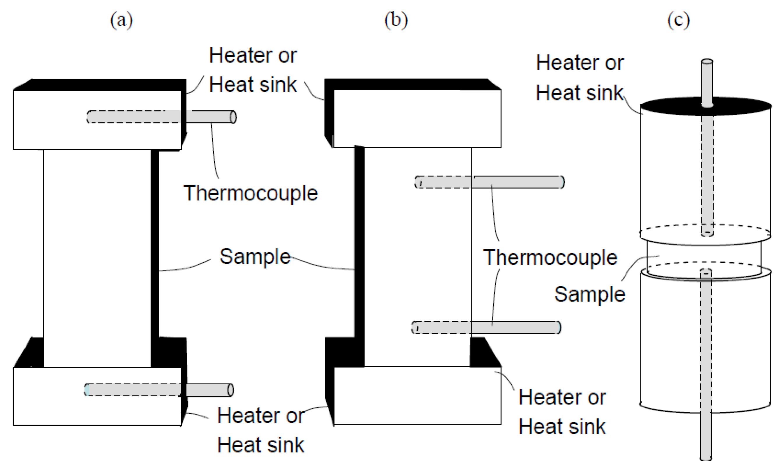
  • The uniaxial 4-point geometry of their apparatus allowed the thermocouples to make direct contact with the sample and produced an isothermal temperature distribution on the surface of the sample.
  • Compressive springs were used to exert a uniform force onto the sample allowing good thermo-mechanical contacts.
  • The spurious Seebeck effects caused by a temperature difference between the voltage probe and the sample were eliminated by using near-zero Seebeck coefficient materials with high thermal conductivity (tungsten and niobium) in the probe in combination with a high Seebeck material in the thermocouple. Lack of co-location in measurements of voltage and temperature.
  • Chemical reactions were eliminated by placing polycrystalline graphite foil between the sample and the thermocouple.
  • An algorithmic approach (delta method) was used to account for the lack of perfect thermal steady state, and correct the thermal drift in the sample.
Figure 1a,b illustrate error prone measurement methods and Figure 1c shows the configuration used by Iwanaga et al. to eliminate these errors.
Figure 1. Three general geometries for measuring the Seebeck coefficient use by Inawaga et al. (a) 2-point geometry where thermocouples are embedded in heater blocks; (b) off-axis 4-point method where thermocouples contact the side of the sample; and (c) Iwanaga et al.’s proposed uniaxial 4-point method. The upper and lower green blocks represent heaters and/or heat sinks, the center block the bulk sample and the narrow rods the thermocouples.
Entropy 15 04700 g001
In Figure 1a the thermoelectric sample is placed between two metal slabs which serve as heat source and sink. In this configuration the thermocouples which are used to measure both temperature and voltage, are embedded in the metal blocks. Measurement errors are produced because of “thermal and electrical contact resistance in these metal blocks themselves as well as across the interfaces between the sample and the metal blocks. In particular the thermal contact resistance may lead to offsets in the temperature measurement.”
In Figure 1b, the sample is placed between the heat source and sink. As Iwanaga et al. state: “The improvement can be understood by analogy to a 2- and 4- point electrical resistance measurement. When measuring materials with low electrical resistance measurement, 4-point measurements are necessary to eliminate the contact resistance errors. Likewise, a 4-point thermal design reduces the effect of thermal contact resistance.” This design, however, is prone to the “cold finger effect” according to which thermocouples can draw heat from the sample, thereby distorting their measurements. This approach also requires that the thermocouples be pressed against the sample with a high force to maintain a good thermal contact. Yet another problem is that the temperature profile at the point of contact is not isothermal.
The configuration used by Iwanaga et al. is shown in Figure 1c. The thermocouples make contact with the sample through the metal blocks. The advantages of this approach are, as these researchers state: “(1) the thermocouples make direct contact to the sample surface; (2) the thermocouple junctions contact an isothermal temperature surface; and (3) the uniaxial design allows thermocouples to exert larger forces onto the sample surface, contributing to the minimization of the thermal and electrical contact resistance.”
The results for the Seebeck measurements are presented as a graph of the voltage response to a temperature differential (Figure 2). The graph clearly shows an offset in the data. The Seebeck curve crosses the X and Y coordinates away from the origin indicating a voltage when the temperature difference is zero (Y intercept), and a temperature difference when the voltage is zero (X intercept). This bias was confirmed in a private communication between the researchers and this author.
Figure 2. Voltage response to temperature gradient has an offset as predicted by the theory.
Entropy 15 04700 g002
Iwanaga et al. assert the lack of an explanation for the observed bias in the data:
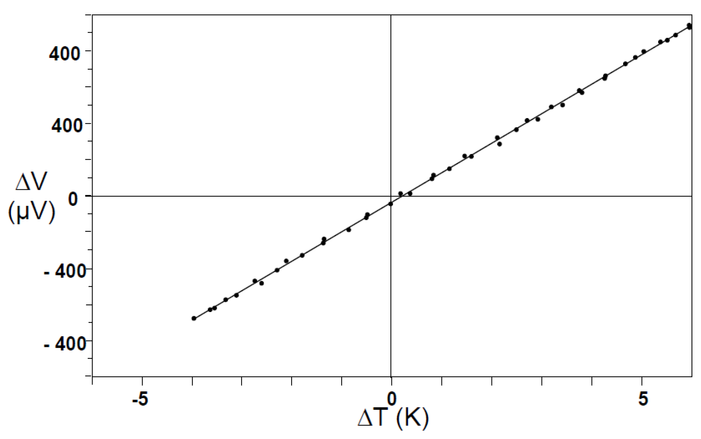
  • “During high temperature measurements, there is often a noticeable voltage offset, which can range from a few µV due to the electronics to almost 1mV, which can sometimes be observed at high temperatures. The origin of the large offset and its effect on the accuracy of the measured Seebeck coefficient is unknown.
Snyder [18], also an author of this set of experiments, makes the following statement:
  • “we and many other thermoelectric groups have observed a temperature offset at zero voltage difference in an attempt to measure Seebeck voltage across thermoelectric samples…. This is commonly observed and subtracted in Seebeck measurement systems including those sold commercially. An offset of about 0.1 K is clearly visible in the paper we published on the measurement of Seebeck coefficient in 2011. This temperature offset can vary greatly and depends on temperature and the type of material tested, and not simply due to errors in thermometry. I have had no less than three students and postdocs study this effect and have collected much data that characterizes it but none have been able to explain this effect.

2.2. Experiment 2

Another series of experiments also performed by Snyder [19] measured a peak voltage of 12 μ across a thermoelectric p+/p junction when the temperature difference between the two sides of the junction was forcibly (or actively) clamped to zero. This voltage was measured for various temperatures as illustrated in Figure 3.
Figure 3. Clamping the temperature to zero across a junction produces a voltage.
Entropy 15 04700 g003
The figure shows that as the temperature is increased from 320 K, the voltage decreases linearly until it reaches a minimum of −12 μV at 380 K. Above 380 K, the junction seems to experience a phase transition or a discontinuity in its operation, possibly a quantum step increase in coupling between the charge carriers and the solid matrix resulting in a sharp decrease in electrical conductivity.
This second experiment confirms the result obtained by the first experiment. A voltage that peaks at −12 μV can be measured across the sample even though the temperature across the sample is zero (Y intercept in Figure 1),
Snyder asserts the lack of a conventional explanation for this effect. He states in a private communication [19]:
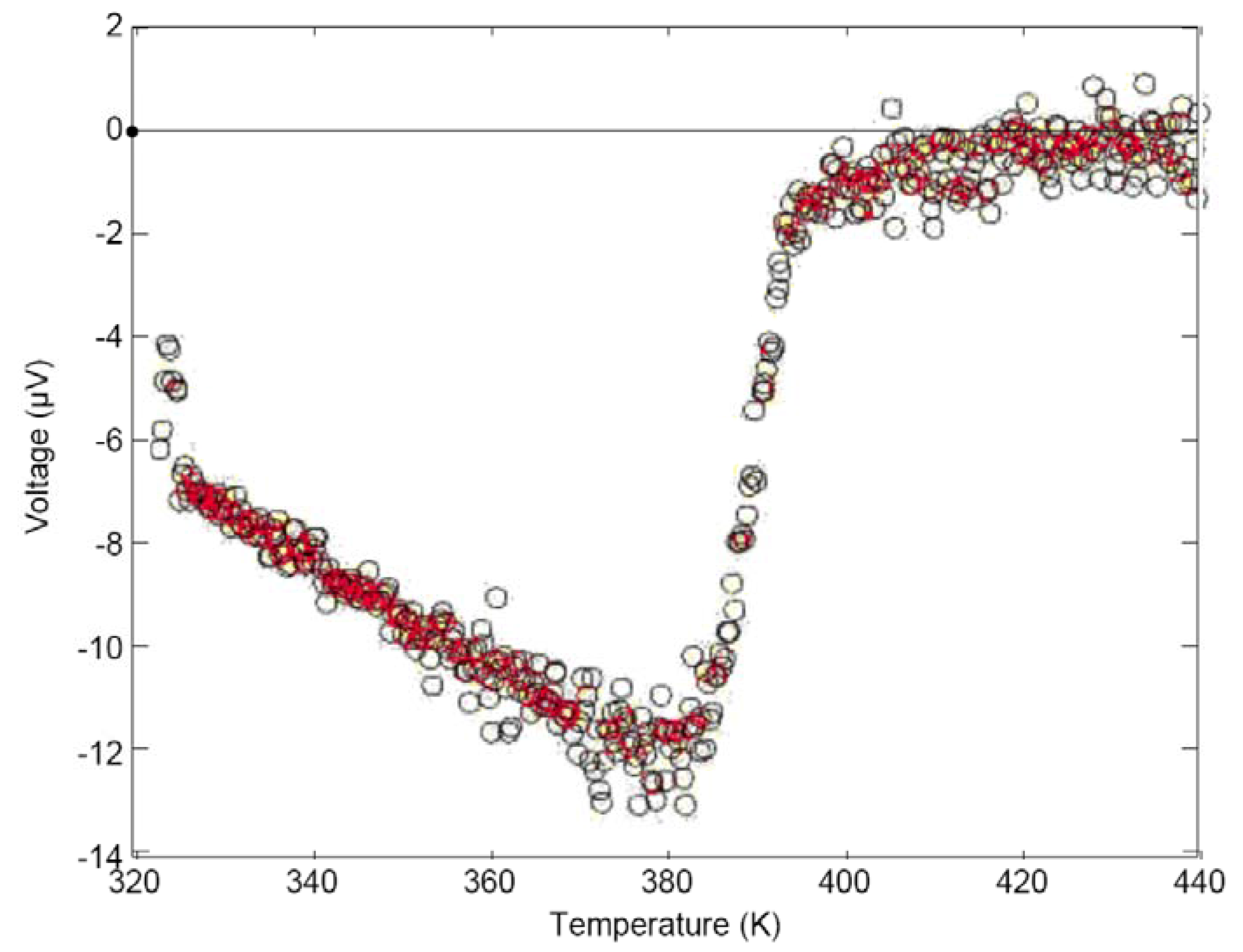
  • “We have no conventional explanation for this effect. From the extent of the data it is clearly reproducible and a property of the material tested because of the known transition in the material at 390K.

3. Theoretical Explanation

3.1. Known Adiabatic Phenomena in Semiconductors

Before advancing the theory behind the observed anomalous results, it is instructive to present known thermoelectric effects as phenomena produced by electrical carriers behaving as if they were in a gas phase [20,21]. As the electrons move in the semiconductor from one region to another with a different Fermi energy level, they undergo a change in temperature, like air being adiabatically compressed or expanded as it changes altitude. This phenomenon is at the core of thermoelectric effects. The Peltier effect [22], (the change in temperature across a junction occurring when a current is flowing) corresponds to the adiabatic cooling or heating of a gas as it is compressed or expanded. The Seebeck effect [23,24,25,26] (the generation of a voltage across a junction subjected to a temperature differential), corresponds to a differential pressure (leading to convection currents) produced when a gas is non-uniformly heated.

3.2. Build-in Properties across Junctions

Semiconductor junctions comprise two built-in properties. The first is the well-known built-in potential which is typically produced when two semiconductor crystals with different doping densities are in contact with each other. The built-in potential is a direct consequence of the Fermi-Dirac distribution [20]:
f ( E ) = 1 1 + e ( E E F ) / k B T
and is given by:
V b i = k B T q ln ( N A N D p o n o )
where NA and NB are the doping densities for acceptor and donor atoms respectively, p0 and n0 are the equilibrium concentration of free charges, T is the temperature, q is the carrier charge and kB is Boltzmann constant.
Even though this potential is responsible for the junction’s electrical properties, it cannot be exploited to produce energy because the electrical connections between two sides of the junction undergo exactly the same drop in potential as the junction itself and any electrical engine or measuring instrument connected across a junction would have an input voltage of exactly zero. The built-in potential can be likened to the pressure differential between different depths in the ocean. This ocean pressure differential cannot be exploited for energy production simply because the pipes connecting a turbine to two different ocean depths would generate a counter pressure exactly canceling the differential pressure between the different depths.
There is another built-in property, not often recognized, which is the converse of the built-in potential. It is the temperature drop of the carriers across a potential barrier in a semiconductor. This effect is a direct consequence of the potential barrier and analogous to the atmospheric adiabatic temperature lapse—that is the drop in temperature of the air with altitude. As illustrated in Figure 4, any carrier climbing the potential energy barrier (by diffusion) loses kinetic energy and, vice versa, any carrier going down the barrier gains energy.
Figure 4. Potential barrier in a semiconductor showing equipartition of energy between potential energy and kinetic energy.
Entropy 15 04700 g004
The Fermi-Dirac distribution implies that across a junction with a potential energy ∆W, the voltage Vbi and the temperature ∆T are related according to:
V b i = k B Δ T q
Substituting the potential energy barrier ∆W = qVbi, the above equation can be rewritten as
Δ T = Δ W / k B
The field can be intrinsic or extrinsic. It can be created in a number of ways, for example by a doping gradient, an n+/n junction, a p+/p junction, or a Schottky junction. The field can also be externally generated, as in a capacitor, by external electrodes on either sides of, and insulated from, the material. No direct current needs to flow through the slab. The presence of an electrical field is sufficient to generate a temperature gradient.
This equation states that a 300 K temperature drop corresponds to 25.86 mV. The built-in potential across a silicon diode’s junction of about 0.7 V corresponds to a temperature of 8100 K–hotter than the surface of the sun. At first sight, one could argue that such an obviously high temperature gradient has never been observed across a junction and therefore the whole idea of this temperature gradient is flawed. Yet theory indicates that there should be such a gradient.

3.3. Adiabatic Phenomena–An Analogy

Adiabatic phenomena in thermoelectric materials can best be understood by likening them to an analogous adiabatic process in the atmosphere, the temperature drop of air with elevation. This phenomenon is called the atmospheric adiabatic temperature lapse [27,28,29,30,31,32,33,34,35] and is well known in the field of aviation and meteorology. In the real atmosphere many factors contribute to this effect. However one can conceive of an adiabatic atmospheric model devoid of the influence of the sun, the wind, and in which the atmosphere consists of a perfect gas in thermal equilibrium and perfectly static. It can be shown from elementary thermodynamics that such a temperature lapse does exist and is spontaneous. Simply explained: molecules that randomly rise convert their kinetic energy into potential energy and, vice versa, molecules that randomly go down convert their potential energy to kinetic energy. Therefore air must be colder at higher altitudes. Another explanation is that as air rises, it encounters a lower pressure and therefore expands adiabatically. The work generated against the surrounding atmosphere is extracted from the kinetic energy of the gas molecules, and therefore air gets colder. When this process occurs slowly enough it becomes reversible and isentropic. The resulting temperature gradient corresponds to the state of maximum entropy. Even though the bottom is hotter than the top no heat flow occurs. The gas is in thermal equilibrium, no convection current is possible and no useful work can be generated from the gas. Since the heat CpT extracted from one mole of ideal gas must be equal to the change in potential energy M0gz of the gas, the adiabatic change in temperature ∆T with a change in altitude ∆z is given by:
CpT = - M0g ∆z
where Cp is the heat capacity per mole M0. Therefore, the change in temperature is,
T = - (M0g/ Cp) ∆z
This equation shows that ∆T is proportional to the molar weight of the gas and the altitude. In the context of thermoelectric material, as shown in Figure 5, the analogous set of equations governing the temperature of carriers is:
kBT = qV,
Since the electric field E = ∆V/∆z:
T = (q E/ kB) ∆z
The atmospheric analog provides an observable proof that adiabatic temperature gradients do exist. Why haven’t they been observed in semiconductors?
Figure 5. The potential barrier causes a gradient in the carrier’s density and in the carrier’s temperature.
Entropy 15 04700 g005

3.4. Diffusion-Diffusion Heat Flow Model

The reason for the lack of observation of such gradients is the following. In conventional semiconductors (low ZT factor), carriers are strongly coupled to the atoms of the crystal matrix and therefore, remain more or less in a state of thermal equilibrium with them. The carrier mean free path is in the order of nanometers and the thermal energy that carriers gain by traveling along the electrical potential gradient is quickly transmitted to the matrix and vice versa. Any temperature difference developed by carriers across a junction is quickly transmitted to heat phonons in the crystal and these phonons which are not affected by the electrical field, in turn, transmit the heat energy by diffusion from the hot region to the cold region as required by Clausius formulation of the Second Law. Essentially phonons operate as a thermal short circuit.
Heat is carried down the temperature gradient by means of phonons. However, the junction is in temperature steady state. Therefore in accordance with the First Law, there must be a reverse heat flow involving heat carried up the temperature gradient by diffusion of the electrical carriers. Heat flows down the temperature gradient by the phonons and up the gradient by the electrons or holes. Up and down in a cycle. This heat flow is circular and continuous. However, in a conventional semiconductor, no noticeable temperature gradient is observed as the two heat flows cancel each other out. This heat transport mechanism involves two decoupled diffusion processes. The first one is mediated by charge carriers, and the second one, by heat phonons. In conventional semiconductors these two processes are indistinguishable because of the strong coupling between the carriers and the phonons.

3.5. The Diffusion and Drift Model

As an aside, it is interesting to mention the diffusion and drift model. Like the above heat flow phenomenon, the well-known diffusion and drift model for semiconductor junctions entails a circular process. A junction is defined by a gradient in the number of fixed charges in a semiconductor solid matrix. These fixed charges which consist of doping atoms embedded in the crystal, generate an electrical field across the junction. A drift current that arises consisting of electrons or holes moving in response to the electrical field, results in the formation of a gradient in the carrier’s density. A second effect, a diffusion current which runs in the direction opposite to the drift current, re-establishes the uniformity of the carrier’s density by moving carriers down the density gradient. Carriers move in one direction, down the electrical field gradient, and in the other direction down the density gradient round and round. These two currents cancel each other out except when an electrical field is applied to the junction. Let’s take these models seriously. What is the source of energy that feeds these currents? How can heat flow up and down a temperature gradient?

3.6. Thermoelectric Materials

Thermoelectric materials are semiconductors specially selected because of the low coupling between the carriers and the crystal matrix. This property is quantified by the figure of merit, ZT, expressed as:
Z T = σ S 2 T / λ
where S is the Seebeck coefficient, T is the temperature and λ is the thermal conductivity of the material. The quantity σ, which stands for the electrical conductivity of the electrons, is really a proxy for their thermal conductivity, and the ratio σ/λ is really a measure of the thermal conductivity ratio of the electrons to the phonons. In good thermoelectric materials, electrons are strongly coupled to each other but not to the phonons. These materials, therefore, seem to be ideal for observing adiabatic temperature gradients generated by charge carriers in semiconductors as discussed above. It is therefore surmised that the researchers who performed the above experiments observed these gradients.

3.7. Hypothesized Thermoelectric Effects

Accordingly, two thermoelectric phenomena driven by field-induced adiabatic temperature gradients are being hypothesized:
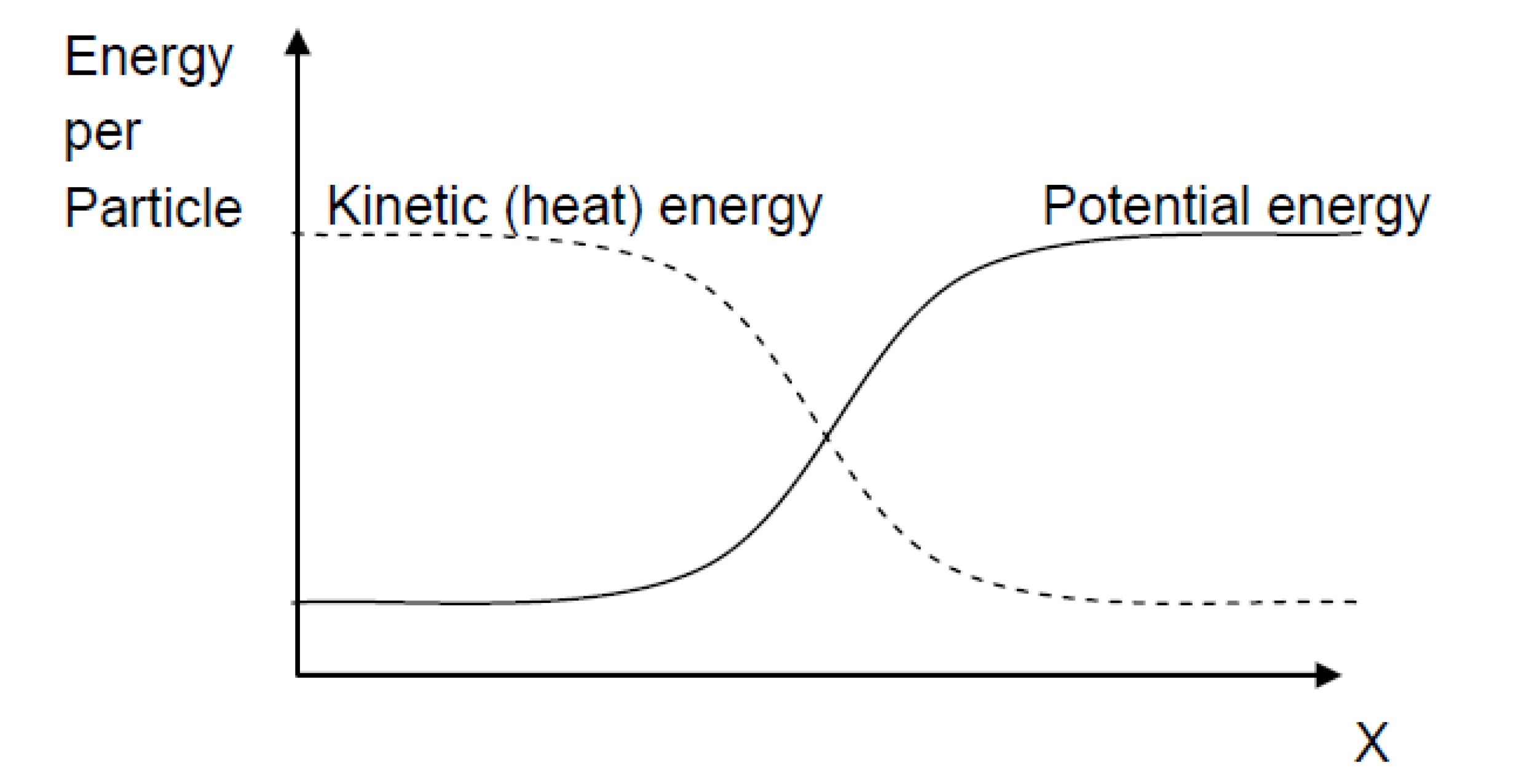
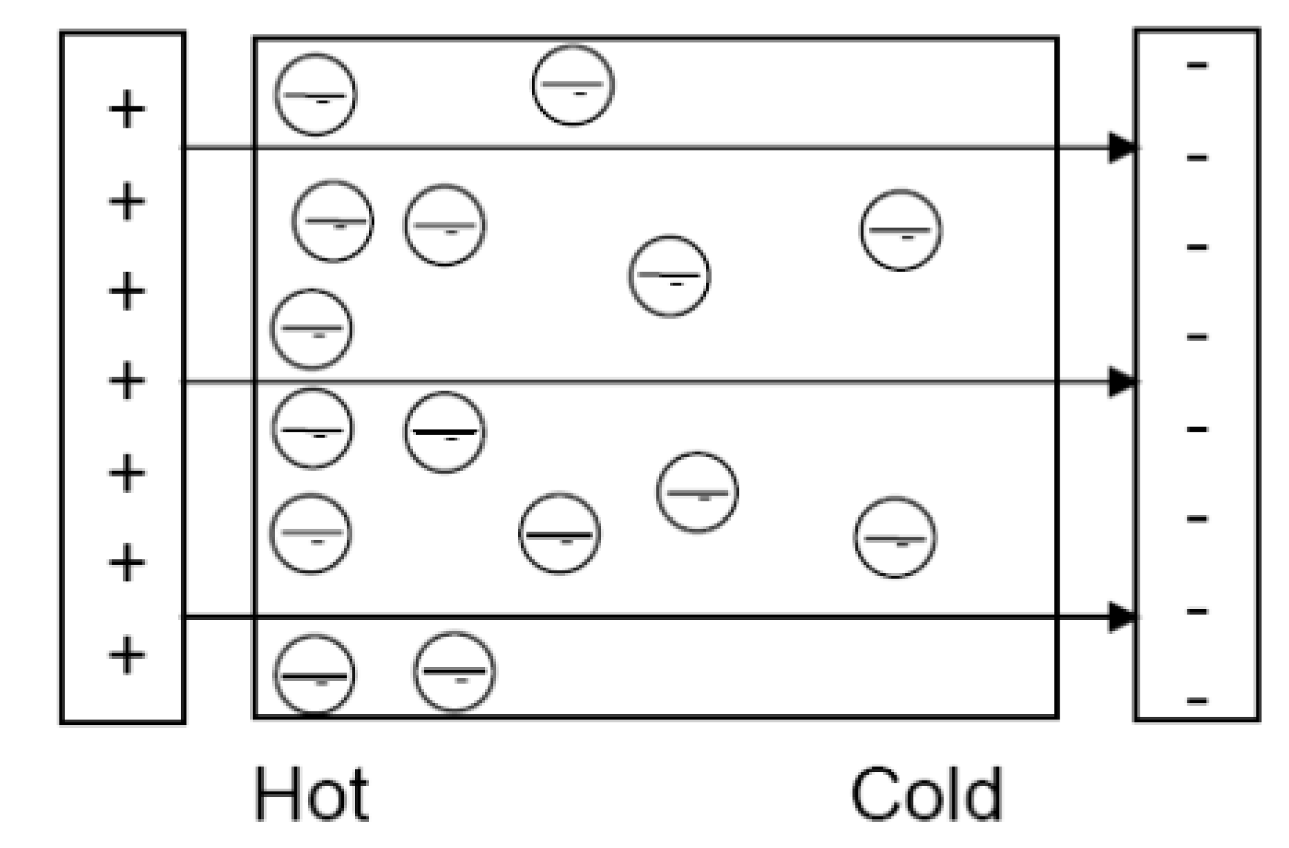
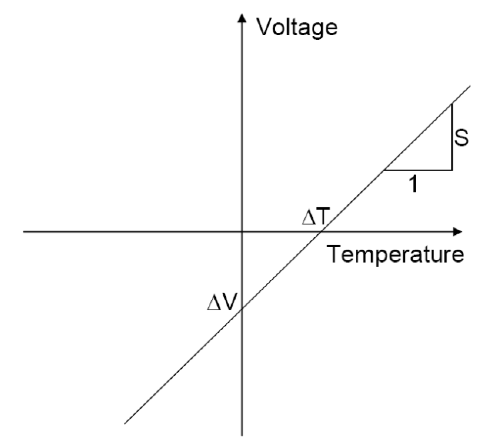
  • An adiabatic temperature difference, ∆T, spontaneously develops across a potential barrier ∆E in a semiconductor in the absence of current or voltage across the barrier. This temperature difference is expected to be most pronounced in materials having a high ratio of thermal conductivity mediated by charge carriers to thermal conductivity mediated by heat phonons. A measure of this ratio is σ/K, the ratio of electrical conductivity to thermal conductivity.
  • Conversely, a voltage ∆V is generated across the barrier if the temperature across the barrier is forcibly clamped to zero, thereby disturbing the temperature profile away from its equilibrium state. This voltage is proportional to the perturbation ∆Tp in the temperature away from its equilibrium state caused by the clamping, and its magnitude can be calculated using the Seebeck coefficient S. Thus:
    Δ V = S Δ T p
This voltage is caused by carriers moving toward the region of the semiconductor whose temperature has been lowered with respect its adiabatic equilibrium state (according to the hot probe phenomenon, carriers move toward the lowest absolute temperature. In this version of the phenomenon, when a temperature gradient is already intrinsic and electro-thermal equilibrium is already established, carriers will move toward the lowest relative temperature, that is, the region which is coolest with respect to the equilibrium profile). These two effects form an Onsager [36,37,38] reciprocal thermoelectric relation of the type described by Callen [39] and are illustrated in Figure 6.
Figure 6. The proposed thermoelectric effects can be represented as intercepts on the axes of a voltage response to a temperature gradient. When ∆V = 0, a temperature ∆T is measured, and when ∆T= 0, a voltage ∆V is measured.
Entropy 15 04700 g006
When a thermoelectric material is subjected to an intrinsic or extrinsic electrical potential three types of heat flow occur:
  • Conventional heat flow mediated by agents such as photons, phonons, or other particles not subjected to the force field. This heat flow occurs in the conventional direction, from hot to cold.
  • Reverse heat flow by diffusion through the electrical carriers subjected to the force field. This heat flow must occur in the reverse direction to counterbalance the forward phonon heat flow and to satisfy the First Law. In high Z thermoelectric materials, this reverse heat flow gives rise to a temperature difference which is not fully cancelled by the forward heat flow because of the low coupling between the carriers and the phonons. This temperature difference becomes observable.
  • Conventional heat flow due to an intentional thermal load such as a thermometer or a thermoelectric generator.

3.7. Heat Conductivity Equation

After a gas phase subjected to a force field reaches thermal equilibrium no heat flow occurs even though a temperature gradient is present. For a molecular gas, Fourier Law of conduction can be corrected by adding a bias term to the gradient:
d Q d t = k ( d T d x + B i a s )
This bias is actually the lapse rate of the gas (equation 6). Fourier’s Law of conduction can then be written as:
d Q d t = k ( d T d x M o g C p )
The equivalent equation for a gas phase in a semiconductor (see Equation (8)) comprised of electrons or holes is
d Q d t = k ( d T d x + q E k B )
where q is the charge of the particle, E is the electrical field and kB is Boltzmann constant.
In practice the temperature bias qE / kB in a semiconductor is partially short-circuited by phonons. If Cc is the thermal conductivity of the electrical carriers and Cp, the thermal resistivity of the phonons, the bias is attenuated by the conductivity ratio:
B i a s = ( q E k B ) ( C c C c + C p )
where Cc + Cp = λ, the thermal conductivity of the material which is used to express the ZT figure of merit. (see equation (9)). If a thermal load such as a thermometer or a heat engine with a conductivity of CL is connected across the semiconductor, the bias is further reduced to
B i a s = ( q E k B ) ( C c C c + C p + C L )
and Equation (13) becomes:
d Q d t = k [ d T d x + ( q E k B ) ( C c C c + C p + C L ) ]
The above equation clearly indicates that no temperature bias can be observed in a semiconductor when Cc << Cc + Cp + CL which is usually the case except in thermoelectric materials as is confirmed by the data collected by Iwanaga et al, and Snyder.

3.8. Seebeck Equation

The bias term applied to the temperature gradient in Equations (14) or (15) can be used to calculate a bias temperature for a given ∆x assuming a uniform field. Since E = dV/dx. The bias temperature Tb for ∆x is:
T b = ( q Δ V k B ) ( C c C c + C p + C L )
This temperature bias term can be incorporated into the Seebeck equation which in its original form is:
Δ V = S Δ T
where the Seebeck coefficient S relates the voltage ∆V to the temperature ∆T across a thermoelectric material. The corrected Seebeck relation is:
Δ V = S ( Δ T + T b )
The above equation states that for a zero temperature difference (∆T = 0,) the voltage ∆V = S Tb can be observed and when the sample is electrically short circuited (∆V = 0) a temperature ∆T = −Tb can be observed.

4. Discussion of Experimental Results

4.1. Discussion of Experiment 1

The experimental graph of Figure 1 is clearly matched by the theoretical prediction of Figure 5. The Seebeck coefficient is 80 µv/K. The adiabatic temperature gradient generates a temperature of 0.3 K at 0 volts (X intercept) indicating that the heat phonons cannot completely short circuit the carrier’s adiabatic gradient. Forcing the temperature to zero, generates a voltage of 24 µv (Y intercept) in accordance with the Seebeck coefficient.

4.2. Discussion of Experiment 2

The graph in Figure 2 comprises a highly non-linear step on the right hand side probably caused by a decrease in the mobility of the carrier above 390K.
The left side of the graph presents a linear increase in the magnitude of the voltage with the temperature of the sample. This behavior can be explained by the Steinhart–Hart equation [40].
1 T = A B ln ( σ ) C ( ln ( σ ) ) 3
where σ is the electrical conductivity of the material. As the temperature increases, σ increases which results in a stronger Seebeck effect as expressed by Equation (7). The curve appears linear because the temperature range is restricted to a small interval.
The experiment indicates that a voltage of 12 µv is generated even though the temperature difference across the sample is zero. The Seebeck coefficient of the sample was approximately 80 μV/K which implies that the temperature gradient across the sample was disturbed by about 12/80 = 0.15 K. In other words, if the junction had not been thermally clamped, it would have experienced a temperature difference of 0.15 K. Clamping generated a temperature perturbation of 0.15 K relative to the equilibrium thermal state, leading to a Seebeck generation of 12 μV.
Using Equation (19), and setting ∆T = 0 (heat clamping) and S = 80 μV/K, generates the bias temperature Tb = 0.15 K. The conductivity ratio in (17) can now be calculated. Iwanaga et al. and Snyder did not state what materials they used in their experiments and therefore the built-in potentials ∆V are not available. Assuming ∆V = 0.7 volts (silicon), q = −1 (electron) and kB = 8.6173324(78) × 10−5 eV/K, Equation (17) yields the conductivity ratio:
C c C c + C p + C L = 1.8 × 10 5
In other words, the thermal conductivity of the electrical carriers is five orders of magnitude lower than that of the phonons and the thermal load combined. This ratio is small but still sufficiently large to have been experimentally observed by Iwanaga et al., and Snyder [17,18,19].
Since a voltage measurement entails a current flow and extraction of power from the samples being tested, one must conclude that, in both sets of experiments described above, ambient heat in the samples was converted to electrical energy by a thermally short-circuited device in accordance with the First Law (notwithstanding the validity of the new thermoelectric effects presented in this paper).

4.3. Discussion of the Theory

As stated by the experimentalists the temperature effects discussed in this paper have been repeatedly observed by many researchers and usually attributed to faulty experimental procedures but these temperature effects have never been credited to adiabatic temperature gradients–probably because of the controversial nature of this assertion. This controversy was initiated in the late 19th century by Loschmidt and Whiting [14,15] and has never been resolved. Essentially the issue revolves around whether an adiabatic temperature gradient can arise spontaneously in a gas column subjected to a gravitational field, or, in the thermoelectric analog, whether an adiabatic temperature gradient can be generated by electrical carriers in a semiconductor subjected to an electrical field. Also in question are the associated thermodynamics effects that would be expected to emerge from such an adiabatic gradient. Such a gradient can readily be observed as a naturally and spontaneously occurring drop in temperature of the atmosphere with elevation.

4.4. Adiabatic Temperature Profile Simulation

The reader is encouraged to download a simulation program provided to the public by this author to perform experiments with a gas subjected to a force field. The program allows the user to observe the spontaneous formation of adiabatic temperature profiles in simulated gas molecules. It also permits the application of thermal perturbations to the temperature profile and lets the user observe the resulting heat flow and the direction of the heat flow as the adiabatic profile restores itself. Of particular interest is the spontaneous occurrence of an adiabatic temperature profile and the associated heat transfer that follows an initial isothermal state. The simulation package is a zip file containing an executable Visual Basic® file, a Microsoft library program for Visual Basic® and a User Manual describing suggested experiments. It can be downloaded from the Entropic Power web site [41].

4.5. Suggestion for Further Research

Biases in Seebeck devices have been viewed in the past as nuisances to be eliminated and/or calibrated out. In fact, research effort should be allocated to maximize these biases either through the selection of materials or the geometry of the devices as these biases present new opportunities in designing novel thermoelectric devices.
Adiabatic temperature gradients are ubiquitous. They arise whenever a force field acts on a gas phase, for example, gravity at the surface of the Earth, the electric field in a semiconductor, or van der Waals forces on the surface of a solid in contact with a gas. These gradients offer a rich source of research opportunities in a wide range of thermodynamics applications.

5. Conclusions

A heat transport mechanism has been formulated to elucidate unexplained experimental data. Two new thermoelectric effects have been identified. The first is the existence of a temperature gradient across a potential barrier in a semiconductor in the absence of any current across the barrier. This gradient is caused by the spontaneous adiabatic distribution of the electrical carriers in the semiconductor.
The second effect is the presence of a measurable voltage across a junction when the temperature gradient is forced to zero by a thermal clamp. This effect is the Onsager reciprocal of the first and is an extension of the hot probe phenomenon in which carriers move toward the lowest relative temperature, that is, the region which is coolest with respect the equilibrium adiabatic profile. The experimental data obtained, but so far, unexplained, was presented as proof that such effects do exist. Suggested future research includes strategies for maximizing and utilizing these effects.

Acknowledgments

I would like to thank Daniel Sheehan for his encouragement, guidance and invaluable suggestions.

Conflicts of Interest

The author declares no conflict of interest.

References and Notes

  1. Thomson, W. On the mechanical theory of thermo-electric currents. Trans. R. Soc. Edinburgh: Earth Sci. 1851, 3, 91–98. [Google Scholar]
  2. Rayleigh, L. On the thermodynamic efficiency of the thermopile. Philos. Mag. Ser. 5 1885, 20, 361–363. [Google Scholar] [CrossRef]
  3. Tolman, R.C.; Fine, P.C. On the irreversible production of entropy. Rev. Mod. Phys. 1948, 20, 51–57. [Google Scholar]
  4. Callen, H.B. The Application of onsager’s reciprocal relations to thermoelectric, thermomagnetic, and galvanomagnetic effects. Phys. Rev. 1948, 73, 1349–1358. [Google Scholar] [CrossRef]
  5. Callen, H.B. On the Theory of Irreversible Processes. Ph.D. Thesis, Massachusetts Institute of Technology—(M.I.T.), Cambridge, MA, USA, 1947. [Google Scholar]
  6. Callen, H.B.; Welton, T.A. Irreversibility and generalized noise. Phys. Rev. 1951, 83, 34–40. [Google Scholar] [CrossRef]
  7. Callen, H.B.; Greene, R.F. On a theorem of irreversible thermodynamics. Phys. Rev. 1952, 86, 702–710. [Google Scholar] [CrossRef]
  8. Callen, H.B. Thermodynamics; John Wiley & Sons, Inc.: New York, NY, USA, 1960. [Google Scholar]
  9. De Groot, S.R. Thermodynamics of Irreversible Processes; North-Holland Publishing Company: Amstedam, The Netherlands, 1963. [Google Scholar]
  10. Fieschi, R.; Groot, S.D.; Mazur, P.; Vlieger, J. Thermodynamical theory of galvanomagnetic and thermomagnetic phenomena II: Reciprocal relations for moving anisotropic mixtures. Physica 1954, 20, 245–258. [Google Scholar] [CrossRef]
  11. Fieschi, R.; Groot, S.D.; Mazur, P. Thermodynamical theory of galvanomagnetic and thermomagnetic phenomena. I: Reciprocal relations in anisotropic metals. Physica 1954, 20, 67–76. [Google Scholar] [CrossRef]
  12. Fieschi, R.; Groot, S.D.; Mazur, P. Thermodynamical theory of galvanomagnetic and thermomagnetic phenomena III: Explicit expressions for the measurable effects in isotropic metals. Physica 1954, 20, 259–273. [Google Scholar] [CrossRef]
  13. De Groot, S.; van Kampen, N. On the derivation of reciprocal relations between irreversible processes. Physica 1954, 21, 39–47. [Google Scholar] [CrossRef]
  14. Capeck, V.; Sheehan, D. Challenges to the Second Law of Thermodynamics; Springer: Norwell, MA, USA, 2005; ISBN 1-4020-3015-0(HB). pp. 202–203. [Google Scholar]
  15. Trupp, A. Energy, entropy: on the occasion of the 100th anniversary of Loschmidt’s death in 1895: Is Loschmidt’s greatest discovery waiting for its discovery? Phys. Essays 1999, 12, 614–628. [Google Scholar] [CrossRef]
  16. Martin, J.; Tritt, T.; Uher, C. High temperature seebeck coefficient metrology. J. Appl. Phys. 2010, 108, 121101. [Google Scholar] [CrossRef]
  17. Iwanaga, S.; Toberer, E.S.; LaLonde, A.; Snyder, G.J. A high temperature apparatus for measurement of the Seebeck coefficient. Rev. Sci. Instrum. 2011, 82, 063905-1–063905-6. [Google Scholar] [CrossRef] [PubMed]
  18. Snyder, Jeoffrey; Material Science, Caltech. Private communication on 20 January 2012.
  19. Snyder, Jeoffrey; Material Science, Caltech. Private communication on 9 April 2012.
  20. Von Zeghbroeck, B. Principles of Semiconductor Devices; Oxford University Press: New York, NY, USA, 2006; Available online: ecee.colorado.edu/~bart/book/book/ (accessed on 24 January 2013).
  21. Goupil, C.; Seifert, W.; Zabrocki, K.; Müller, E.; Snyder, J. Thermodynamics of thermoelectric phenomena and applications. Entropy 2011, 13, 1481–1517. [Google Scholar] [CrossRef]
  22. Peltier, J.C.A. Nouvelles expériences sur la caloricité des courants électriques. Ann. Chim. Phys. 1834, 56, 371–386. [Google Scholar]
  23. Seebeck, T.J. Ueber den Magnetismus der galvenischen Kette; Technical Report for the Royal Prussian Academy of Science: Berlin, Germany, 1821. [Google Scholar]
  24. Seebeck, T.J. Magnetische Polarisation der Metalle und Erze durch Temperatur-Differenz; Technical Report for the Royal Prussian Academy of Science: Berlin, Germany, 1823. [Google Scholar]
  25. Seebeck, T.J. Ueber die magnetische polarisation der metalle und erze durch temperatur-differenz. Annalen der Physik 1826, 82, 1–20. [Google Scholar] [CrossRef]
  26. In fact, Seebeck mistook the observed effect as a thermomagnetic coupling. The correct interpretation was later provided by Oersted.
  27. Jacobson, M.Z. Fundamentals of Atmospheric Modeling, 2nd ed.; Cambridge University Press: New York, NY, USA, 2005. [Google Scholar]
  28. Donald Ahrens, C. Meteorology Today, 8th ed.; Brooks/Cole Publishing: Belmont, CA, USA, 2006. [Google Scholar]
  29. Glickman, T.S. Glossary of Meteorology, 2nd ed.; American Meteorological Society: Boston, MA, USA, 2000. [Google Scholar]
  30. Salomons, E.M. Computational Atmospheric Acoustics, 1st ed.; Springer: Secaucus, NJ, USA, 2001. [Google Scholar]
  31. Stull, R.B. An Introduction to Boundary Layer Meteorology, 1st ed.; Kluwer Academic Publishers: Dordrecht, The Netherlands, 1988. [Google Scholar]
  32. Calvert, J.G. Glossary of Atmospheric Chemistry Terms Atmospheric Chemistry Division, National Center for Atmospheric Research, page 2171. In Pure&App/. Chem.; Vol. 62, No. 11; Boulder, CO, USA, 1990. [Google Scholar]
  33. Danielson, E.W.; Levin, J.; Abrams, E. Meteorology; McGraw Hill: Dubuque, Iowa, IA, USA, 2003. [Google Scholar]
  34. Fluid mechanics. In Course of Theoretical Physics, Volume 6; Landau, L.D.; Lifshitz, E.M. (Eds.) Pergamon Press: New York, NY, USA, 1982.
  35. Fronsdal, C. Heat and Gravitation. I. The Action Principle. 2011. [Google Scholar] [CrossRef]
  36. Onsager, L. Reciprocal relations in irreversible processes. I. Phys. Rev. 1931, 37, 405–426. [Google Scholar] [CrossRef]
  37. Onsager, L. Reciprocal relations in irreversible processes. II. Phys. Rev. 1931, 38, 2265–2279. [Google Scholar] [CrossRef]
  38. Onsager, L. Theories and problems of liquid diffusion. Ann. N. Y. Acad. Sci. 1945, 46, 241–265. [Google Scholar] [CrossRef] [PubMed]
  39. Callen, H.B. The application of Onsager’s reciprocal relations to thermoelectric, thermomagnetic, and galvanomagnetic effects. Phys. Rev. 1948, 73, 1349–1358. [Google Scholar] [CrossRef]
  40. Steinhart, J.S.; Hart, S.R. Calibration curves for thermistors. Deep Sea Res. Oceanogr. Abstr. 1968, 15, 497–503. [Google Scholar] [CrossRef]
  41. Entropic Power, Simulator. Available online: http://www.entropicpower.com/simulation (accessed on 24 October 2013).

