Wavelet q-Fisher Information for Scaling Signal Analysis

Abstract

This article first introduces the concept of wavelet q-Fisher information and then derives a closed-form expression of this quantifier for scaling signals of parameter α. It is shown that this information measure appropriately describes the complexities of scaling signals and provides further analysis flexibility with the parameter q. In the limit of $q\to 1$, wavelet q-Fisher information reduces to the standard wavelet Fisher information and for $q>2$ it reverses its behavior. Experimental results on synthesized fGn signals validates the level-shift detection capabilities of wavelet q-Fisher information. A comparative study also shows that wavelet q-Fisher information locates structural changes in correlated and anti-correlated fGn signals in a way comparable with standard breakpoint location techniques but at a fraction of the time. Finally, the application of this quantifier to H.263 encoded video signals is presented.

1. Introduction

The study of the properties of computer network traffic is important for many aspects of computer network design, performance evaluation, network simulation, capacity planning, network algorithmic design, among others. In the very beginning of computer network traffic modelling, the traffic itself was considered Markovian (with Poisson arrivals), because older telephone network traffic was suitably described by this model and thus it was unsurprising to consider the characteristics of network traffic similar to that of the telephone network. Markovian models permitted straightforward computations of performance issues due to its short-range dependent (SRD) nature and because of the ease of computation and lack of memory, they became very popular. The modelling of computer network traffic with Markovian models ended when Leland and co-workers [1,2], based on detailed studies of high-resolution network measurements, discovered that network traffic did not follow the Markovian model but instead it was more appropriately modeled by self-similar or fractal stochastic processes. Subsequent studies not only validated this finding but also found self-similar features in additional network configurations [3,4] and traffic expected to flow in future networks [5,6]. The self-similar nature of network traffic (local area network (LAN), Delay, variable-bit rate (VBR) video, etc.) indicated that computer network traffic behaves “statistically" similar at different scales of observation. As a matter of fact, persistence behavior was observed in LAN traffic at small as well as on high levels of observation. This finding was contrary to commonly observed features of Markovian models where for large scales the traffic appeared to reduce to white noise. The self-similar nature of network traffic implied that numerous results based on the Markovian model needed to be thoroughly revised. Later, many authors reported that when considering traffic as a self-similar process, many Internet quality of service (QoS) metrics such as delay, packet-loss rate and jitter increased. This performance degradation implied that based on the observed characteristics, not only was it necessary to characterize the traffic flowing through a network, but also specifically designed actions were required to maintain the QoS of the network at acceptable levels.

The characterization of traffic was in principle performed by estimating the parameters which determine most of its properties and behavior. The Hurst parameter (or the self-similarity parameter) provided a rather complete characterization of self-similar processes. However, due to the complex characteristics of observed traffic, nowadays it is clear that complementary techniques are required [7,8,9]. Self-similar processes are related to long-memory, fractal and multifractal processes and it is common to find in the scientific literature claims that traffic is self-similar, fractal or multifractal. Self-similar processes along with long-memory, fractal, $1/f$ and multifractal processes belong to the class of scaling or scale-invariant signals. The theory of scaling signals has been relevant for the study of many phenomena occurring in diverse fields of science and technology. Some aspects of physiology such as heart-rate variability [10] are suitably modeled by scaling signals and the parameter estimated from scaling signals determines much of the properties of the heart and the individual under study [10]. Electroencephalogram (EEG) signals obtained in humans and animals are also appropriately described by scaling signals [11]. They also model the traffic flowing through computer communications [3,12,13], the turbulence in physics, the noise observed in electronic devices [14] and the time series obtained in economy [4] and finance, among others.

Many techniques and methodologies have been proposed to analyze these processes [15,16,17]; however, they have shown to be limited for the rich set of complexities observed in the data [8,18]. Moreover, many articles have concluded that no single technique of analysis is sufficient for providing efficient and robust estimation of the scaling parameter [15]. Because of this, current works concentrate on developing cutting-edge techniques that are robust to trends, level-shifts and missing values embedded in the data under study. The presence of these phenomenologies significantly impact the estimation process and can lead to misinterpretation of the phenomena [10,15]. In this context, recent results which attempt to study the complexities of the underlying process using wavelet based entropies provide interesting alternatives. As a matter of fact, it has been demonstrated, for example, that wavelet Tsallis q-entropies behave as a sum-cosh window [9] and that this behavior can be used to detect multiple mean level-shifts embedded in the scaling signal under study and for the classification of scaling signals as stationary or non-stationary as well [18].

This article defines the concept of wavelet q-Fisher information and shows that this information quantifier can be used for the important problem of detecting level-shifts embedded in scaling signals, in particular to H.263 signals. Closed-form expressions are found for the wavelet q-Fisher information of scaling signals and information planes are also constructed. Wavelet q-Fisher information generalizes wavelet Fisher information [19] and provides further analysis flexibility with the parameter q. Parameter q in wavelet q-Fisher information permits to adapt the analyses to the type and characteristics of the data. Extensive experimental studies using simulated signals validate the theoretical findings. It is shown that wavelet q-Fisher information not only detects but also locates level-shifts in synthesized fractional Gaussian noise (fGn) signals and H.263 encoded video signals.

The rest of the article is organized as follows, in Section 2, the properties and definitions of scaling signals are briefly studied and its wavelet analysis explored. Some important results are reviewed for fractional Brownian motion (fBm), fGn and discrete pure power-law (dPPL) signals. Section 3 defines the wavelet q-Fisher information concept and derives a closed-form expression (based on the q-analysis) of this quantifier for scaling signals. Information planes are constructed from the theoretical formulas and the behaviors of the quantifiers are explored for a range of the parameter α. The potential applications of wavelet q-Fisher information are also presented in this section. Section 4 details the level-shift detection problem and describes the way in which wavelet q-Fisher information is expected to detect level-shifts embedded in scaling signals. Section 5 presents the level-shift detection properties of wavelet q-Fisher information in synthesized fGn signals and later, a comparative study using correlated and anti-correlated fGn signals is performed using the Bai and Perron [20] algorithm and a version of the Bai and Perron technique along with with wavelet q-Fisher information. The rest of Section 5 presents the analysis of H.263 encoded video signals with wavelet q-Fisher information. Finally, Section 6 presents the conclusion of the article.

2. Wavelet Analysis of Scaling Processes

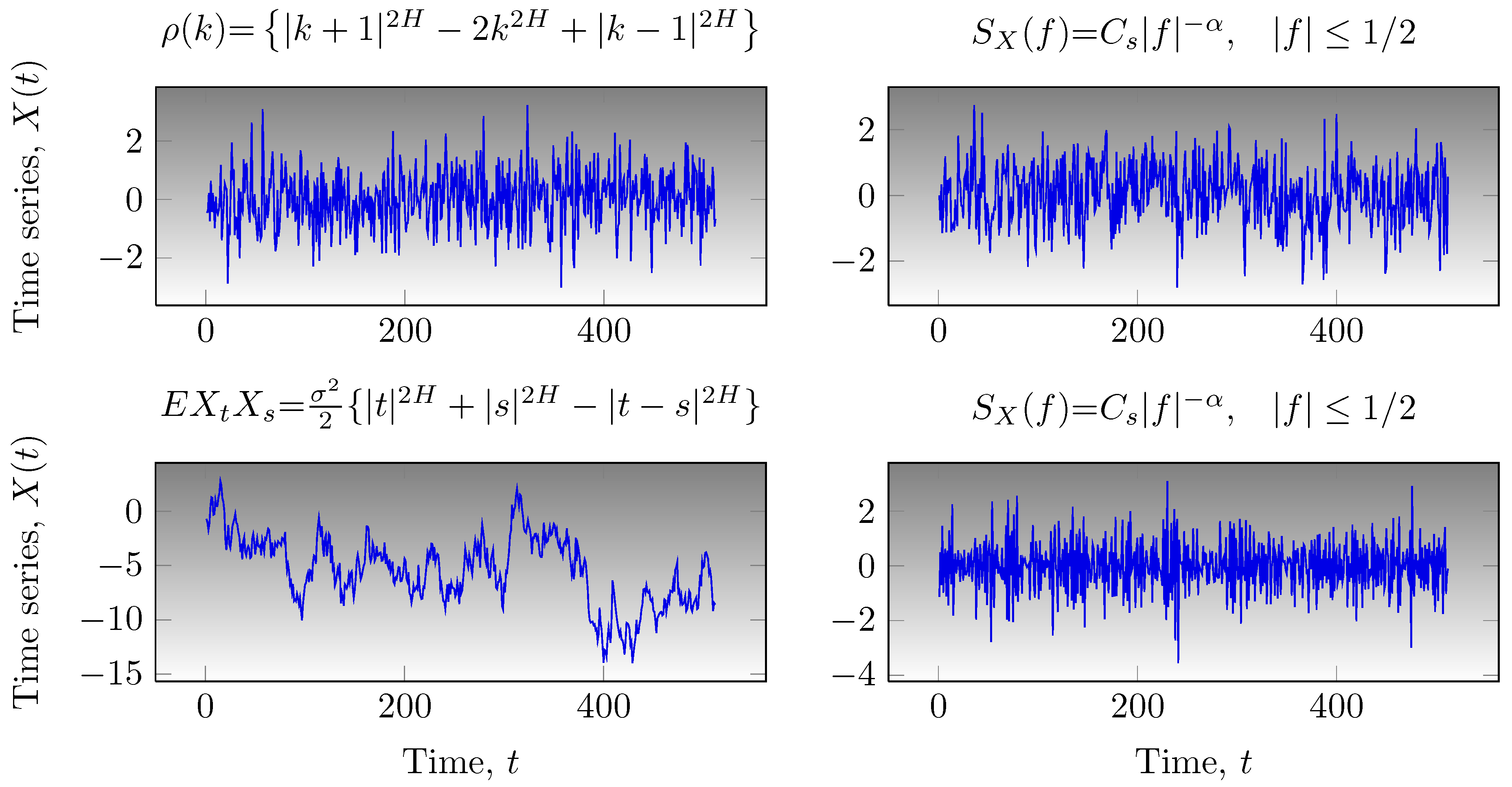
2.1. Scaling Processes

Scaling processes of parameter α, also called $1/f^{\alpha }$ or power-law processes, have been extensively applied and studied in the scientific literature since they model diverse phenomena [12,13] within these fields. These processes are sufficiently characterized by the parameter α, called the scaling-index, which determines many of their properties. Various definitions of the scaling property have been proposed in the scientific literature, some based on their characteristics such as self-similarity or long-memory, others based on the behaviour of their power spectral density (PSD). In this article, a scaling process is a random process for which the associated PSD behaves as a power-law in a range of frequencies [3,21], i.e.,

$$S\left(f\right)\sim c_f{\left|f\right|}^{-\alpha },f\in (f_a,f_b)$$

(1)

where $c_f$ is a constant, $\alpha \in \mathbb{R}$ the scaling index and $f_a,f_b$ represent the lower and upper bound frequencies upon which the power-law scaling holds. Depending upon $f_a$, $f_b$ and α, several particular scaling processes and behaviours can be identified. Independently of α, local regularity and band-pass power-law behaviour is observed whenever $f_a\to \infty$ and $f_b>f_a\gg 0$ respectively. When the scaling-index α is taken into consideration, long-memory behaviour is observed when both $0<\alpha <1$ and $f_b>f_a\to 0$. Self-similar features (in terms of distributional invariance under dilations) are observed in all the scaling-index range for all f. Scaling-index α determines not only the stationary and non-stationary condition of the scaling process but also the smoothness of their sample path realizations. The greater the scaling index α, the smoother their sample paths. As a matter of fact, as long as $\alpha \in (-1,1)$, the scaling process is stationary (or stationary with long-memory for small f and $\alpha \in (0,1)$) and non-stationary when $\alpha \in (1,3)$. Some transformations (e.g., the Lamperti transformation) can make a stationary process appear non-stationary and vice versa. Outside the range $\alpha \in (-1,3)$, several other processes can be identified, e.g., the so-called extended fBms and fGns defined in the work of Serinaldi [15]. The persistence of scaling processes can also be quantified by the index α and within this framework, scaling processes possess negative persistence as long as $\alpha <0$, positive weak long-persistence when $0<\alpha <1$ and positive strong long-persistence whenever $\alpha >1$. Scaling signals encompasses a large family of well-known random signals, e.g., fBms, fGns [22], pure power-law processes [21], multifractal processes [3], etc. FBm, $B_H\left(t\right)$, comprises a family of Gaussian, self-similar processes with stationary increments and because of the Gaussianity, it is completely characterized by its autocovariance sequence (ACVS), which is given by,

$$\mathbb{E}{B}_H\left(t\right)B_H\left(s\right)=R_{B_H}(t,s)=\frac{{\sigma }^2}{2}\left\{{\left|t\right|}^{2H}+{\left|s\right|}^{2H}-{|t-s|}^{2H}\right\}$$

(2)

where $0<H<1$ is the Hurst index. FBm is non-stationary and theoretically no spectrum can be defined on it. However, fBm possesses an average spectrum of the form $S_{\text{fBm}}\left(f\right)\sim c{\left|f\right|}^{-(2H+1)}$ as $f\to 0$ which implies that $\alpha =2H+1$ [23]. FBm appears very often as a model for many non-stationary phenomena; however, when the signal under study is stationary, the fGn process (obtained from a transformation of fBm) is rather used. FGn, $G_{H,\delta }\left(t\right)$, obtained by sampling a fBm process and computing increments of the form $G_{H,\delta }\left(t\right)=1/\delta \{B_H(t+\delta )-B_H\left(t\right)\},\delta \in {\mathbb{Z}}_{+}$ (i.e., by differentiating fBm), is a well-known Gaussian self-similar and long-memory process. The ACVS of this process is given by:

$$\mathbb{E}{G}_{H,\delta }\left(t\right)G_{H,\delta }(t+\tau )=\frac{{\sigma }^2}{2}{\left\{\right|\tau +\delta |}^{2H}{+|\tau -\delta |}^{2H}-{2\left|\tau \right|}^{2H}\}$$

(3)

where $H\in (0,1)$ is the Hurst index. The associated PSD of fGn is given by [21]:

$$S_{\text{fGn}}\left(f\right)=4{\sigma }_X^2{C}_H{sin}^2\left(\pi f\right)\sum _{j=-\infty }^{\infty }\frac{1}{{|f+j|}^{2H+1}}\left|f\right|\le \frac{1}{2}$$

(4)

where ${\sigma }_X$ is the process’ variance and $C_H$ is a constant. FGn is stationary and for large enough τ and under the restriction of $1/2<H<1$ possesses long-memory or long-range dependence (LRD). The scaling index α associated to fGn signals is given by $\alpha =2H-1$ as its PSD, given by Equation (4), behaves asymptotically as $S_{\text{fGn}}\left(f\right)\sim c{\left|f\right|}^{-2H+1}$ for $f\to 0$. Another scaling process of interest is the family of discrete pure power-law processes (dPPL) which are defined as processes for which their PSD behaves as $S_X\left(f\right)=C_S{\left|f\right|}^{-\alpha }\text{for}\left|f\right|\le 1$, where $\alpha \in \mathbb{R}$ and $C_s$ represent a constant. PPL signals are stationary when the power-law parameter $\alpha <1$ and non-stationary whenever $\alpha >1$. As stated in the work of Percival [21], the characteristics of these processes and those of fBms/fGns are similar, however, the differences between fBms and PPLs with $\alpha >1$ are more evident. As a matter of fact, differentiation of stationarity/non-stationarity is far more difficult for PPL than for fBms/fGns. Figure 1 displays some realizations of fGn, fBm and PPL processes. The scaling-index α of the PPL signals are identical to the scaling-index of the associated fGn and fBm. Note that the characteristics of the sample paths of fGn are fairly different from those of fBm. In the case of PPL processes, this differentiation is not so evident and as a matter of fact, when the scaling indexes approach the boundary $\alpha =1$, classification becomes complex. For further information on the properties, estimators and analysis techniques of scaling processes please refer to [3,12,13,15,16,21,24].

Figure 1. Sample path realizations of some scaling processes. Top left depicts a fGn with $\alpha =-0.1$, top right shows a PPL process with $\alpha =-0.1$, bottom left plots a fBm signal with $\alpha =1.9$ and finally, bottom right plots a PPL process with $\alpha =1.9$.

Figure 1. Sample path realizations of some scaling processes. Top left depicts a fGn with $\alpha =-0.1$, top right shows a PPL process with $\alpha =-0.1$, bottom left plots a fBm signal with $\alpha =1.9$ and finally, bottom right plots a PPL process with $\alpha =1.9$.

2.2. Wavelet Analysis of Scaling Signals

Wavelets and wavelet transforms have been extensively applied for the analysis of deterministic and random signals in almost every field of science [8,25,26]. The advantages of wavelet analysis over standard techniques of signal analysis has been widely reported in the literature and its potential for non-stationary signal analysis proven. Wavelet analysis represents a signal $X_t$ in time-scale domain by the use of an analyzing or mother wavelet, ${\psi }_o\left(t\right)$ [27]. For the purposes of the paper, ${\psi }_o\left(t\right)\in L_1\cap L_2$ and the family of shifted and dilated ${\psi }_o\left(t\right)$ form an orthonormal basis of $L_2\left(\mathbb{R}\right)$. In addition, the finiteness of the mean average energy ($\mathbb{E}\int {\left|X\left(u\right)\right|}^{2}du<\infty$) on the scaling process allows to represent it as a linear combination of the form:

$$X_t=\sum _{j=1}^L\sum _{k=-\infty }^{\infty }{d}_X(j,k){\psi }_{j,k}\left(t\right)$$

(5)

where $d_X(j,k)$ is the discrete wavelet transform (DWT) of $X_t$ and $\{{\psi }_{j,k}\left(t\right)=2^{-j/2}{\psi }_o(2^{-j}t-k),j,k\in \mathbb{Z}\}$, is a family of dilated (of order j) and shifted (of order k) versions of ${\psi }_o\left(t\right)$. The coefficients $d_X(j,k)$ in Equation (5), obtained by DWT, represent a random process for every j, a random variable for fixed j and k and as such many statistical analyses can be performed on them. Equation (5) represents signal $X_t$ as a linear combination of L detail signals, obtained by means of the DWT. DWT is related to the theory of multi-resolution signal representation (MRA), in which signals (or processes) can be represented at different resolutions based on the number of detail signals added to the low-frequency approximation signal. This can be written by the following equation

$$X_t=X_L+\sum _{j=1}^L\sum _{k=-\infty }^{\infty }{d}_X(j,k){\psi }_{j,k}\left(t\right)$$

(6)

where $X_L$ is the approximation signal at scale L, which is obtained by projection of $X_t$ in approximation spaces ${\mathcal{V}}_j$, and the right represent the L detail signals obtained by projections of $X_t$ in wavelet spaces ${\mathcal{W}}_j$. In the study of scaling processes, wavelet analysis has been primarily applied in the estimation of the wavelet variance [7,8]. Wavelet variance or spectrum of a random processes accounts for computing variances of wavelet coefficients at each scale. Wavelet variance not only has permitted to propose estimation procedures for the scaling-index α but also to compute entropies and other information measures associated to scaling signals. Wavelet spectrum has also been used for detecting non-stationarities embedded in Internet traffic [8] and has been shown to describe appropriately the second-order properties of some well-known processes. For stationary zero-mean processes, wavelet spectrum is given by:

$$\mathbb{E}{d}_X^2(j,k)={\int }_{-\infty }^{\infty }{S}_X\left(2^{-j}f\right){|\Psi \left(f\right)|}^{2}df$$

(7)

where $\Psi \left(f\right)=\int \psi \left(t\right){\text{e}}^{-j2\pi ft}dt$ is the Fourier integral of ${\psi }_o\left(t\right)$ and $S_X(.)$ represents the PSD of $X_t$. Table 1 summarizes the wavelet spectrum for some standard scaling processes. Note that $\mathbb{E}(.)$ and $\text{Var}(.$) represent the expectation and the variance operator and $C(\psi ,\alpha )$ and C constants. The mathematical properties and the estimation procedures for the class of long-memory, self-similar and Hsssi processes are defined further in the work of Beran [13] and for the class of dPPL signals in the work of Percival [21]. Hsssi processes are signals for which both the self-similarity property and the stationarity of the increments is satisfied. It permits to obtain in the limit a long-memory signal as long as $H\in (1/2,1)$. This process is of fundamental importance since it has stationary properties and as a consequence is extensively used in the literature to model many phenomena. For further details on the analysis, estimation and synthesis of scaling processes, please refer to the works of Abry [27,28], Bardet [29,30] and references therein.

Table 1. Wavelet spectrum or wavelet variance associated to different types of scaling processes. $\mathbb{E}(.)$, $\text{Var}(.)$ and $\Psi (.)$ represent expectation, variance and Fourier integral operators respectively.

Type of scaling process	Associated wavelet spectrum or variance
Long-memory process	$\mathbb{E}{d}_X^2(j,k)\sim 2^{j\alpha }C(\psi ,\alpha )$,   $C(\psi ,\alpha )=c_{\gamma }\int {\left|f\right|}^{-\alpha }{|\Psi \left(f\right)|}^{2}df$
Self-similar process	$\mathbb{E}{d}_X^2(j,k)=2^{j(2H+1)}\mathbb{E}{d}_X^2(0,k)$
Hsssi process	$\text{Var}{d}_X^2(j,k)=2^{j(2H+1)}\text{Var}{d}_X(0,0)$
dPPL process	$\mathbb{E}{d}_X^2(j,k)=C{2}^{j\alpha }$

Table 1. Wavelet spectrum or wavelet variance associated to different types of scaling processes. $\mathbb{E}(.)$, $\text{Var}(.)$ and $\Psi (.)$ represent expectation, variance and Fourier integral operators respectively.

Type of scaling process	Associated wavelet spectrum or variance
Long-memory process	$\mathbb{E}{d}_X^2(j,k)\sim 2^{j\alpha }C(\psi ,\alpha )$,   $C(\psi ,\alpha )=c_{\gamma }\int {\left|f\right|}^{-\alpha }{|\Psi \left(f\right)|}^{2}df$
Self-similar process	$\mathbb{E}{d}_X^2(j,k)=2^{j(2H+1)}\mathbb{E}{d}_X^2(0,k)$
Hsssi process	$\text{Var}{d}_X^2(j,k)=2^{j(2H+1)}\text{Var}{d}_X(0,0)$
dPPL process	$\mathbb{E}{d}_X^2(j,k)=C{2}^{j\alpha }$

3. Wavelet q-Fisher Information of $1/f^{\alpha }$ Signals

3.1. Time-Domain Fisher’s Information Measure

Fisher’s information measure (FIM) has recently been applied in the analysis and processing of complex signals [31,32,33]. In [31], FIM was applied to detect epileptic seizures in EEG signals recorded in human and turtles. Later, the work of Martin [32] reported that FIM can be used to detect dynamical changes in many non-linear models such as the logistic map, Lorenz model, among others. The work of Telesca [33] reported on the application of FIM for the analysis of geoelectrical signals. Recently, Fisher information has been extensively applied in quantum mechanical systems for the study of single particle systems [34] and also in the context of atomic and molecular systems [35]. Fisher’s information measure has also been used in combination with Shannon entropy power to construct the so-called Fisher–Shannon information plane/product (FSIP) [36]. The Fisher–Shannon information plane was recognized in that work to be a plausible method for non-stationary signal analysis and has been applied to study geoelectrical and other nonstationary signals. Let $X_t$ be a random signal with associated probability density $f_X\left(x\right)$. Fisher’s information (in time-domain) of signal $X_t$ is defined according to the following relation

$$I_X=\int {\left(\frac{\partial }{\partial x}{f}_X\left(x\right)\right)}^2\frac{dx}{f_X\left(x\right)}$$

(8)

Fisher’s information $I_X$ is a non-negative quantity that yields large (possibly infinite) values for smooth signals and small values for random disordered data. Accordingly, Fisher’s information is large for narrow probability densities and small for wide (flat) ones [37]. Fisher information is also a measure of the oscillatory degree of a waveform, where highly oscillatory functions have large Fisher information [34]. The purpose of the article is to study the behavior of Fisher information (defined in wavelet domain) of scaling signals of parameter α. Fisher’s information has mostly been applied in the context of stationary signals using a discretized version of Equation (8), which is given by the following equation,

$$I_X=\sum _{k=1}^L\left\{\frac{{\left(p_{k+1}-p_k\right)}^2}{p_k}\right\}$$

(9)

for some probability mass function (pmf) ${\left\{p_k\right\}}_{k=0}^L$. Fisher information can be generalized in various ways to provide further analysis flexibility and to adapt the analyses to the characteristics of the data under study. Several generalizations have been proposed in the literature. This article uses and studies the q-Fisher information of Plastino and coworkers [11]. Plastino and co-workers defined the q-Fisher information of a probability mass functions as [11]

$${\mathcal{I}}_q\equiv \sum _j{\left\{p_{j+1}-p_j\right\}}^2{p}_j^{q-2}$$

(10)

As stated above, parameter q provides further analysis flexibility and can highlight possible nonstationarities embedded in the signal under study. In this context, q-Fisher information is again a descriptor of the complexities associated to random signals and shares similar properties as the standard Fisher’s information in the sense that it is large for narrow probability density and also for highly oscillatory data.

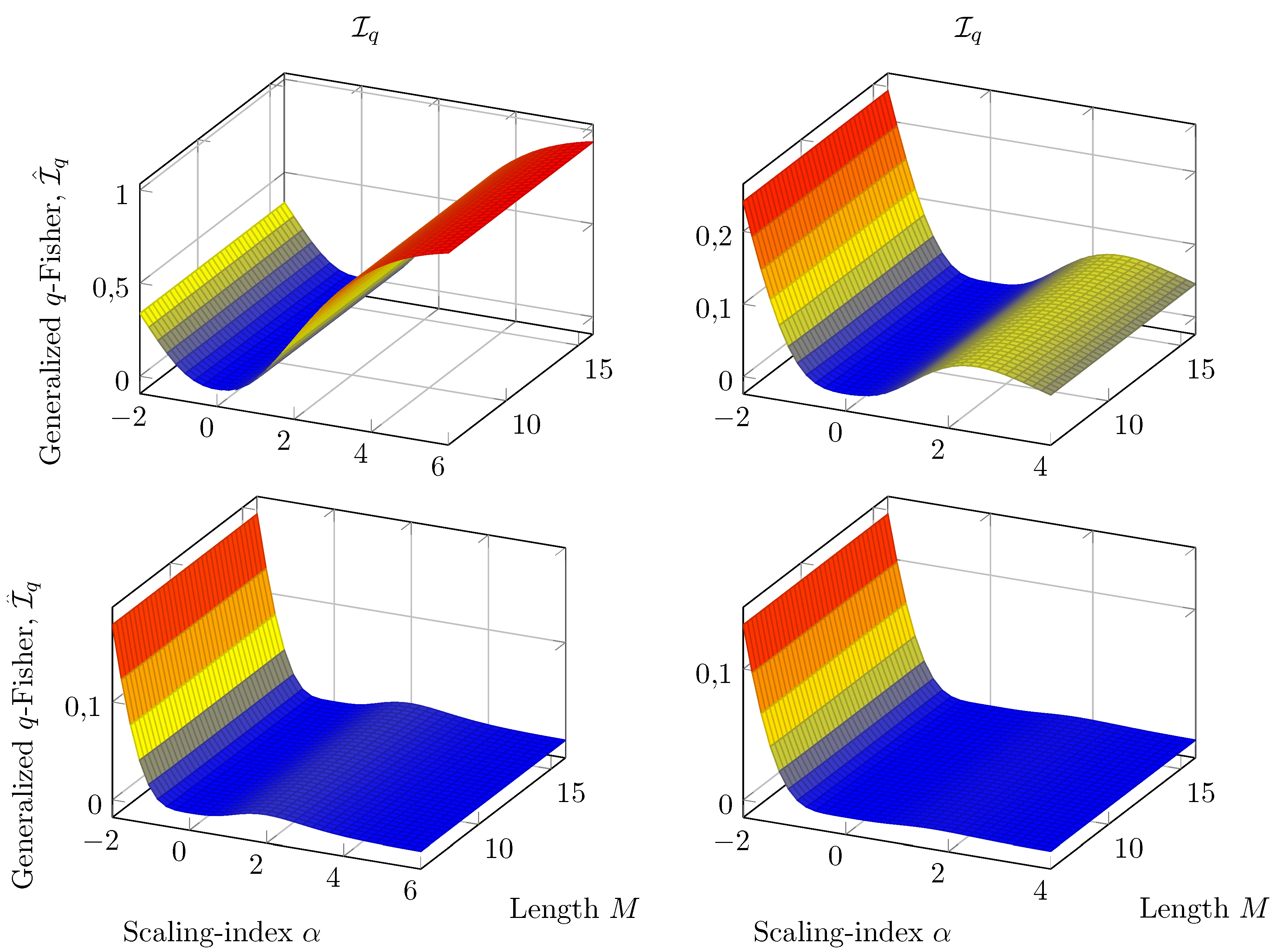
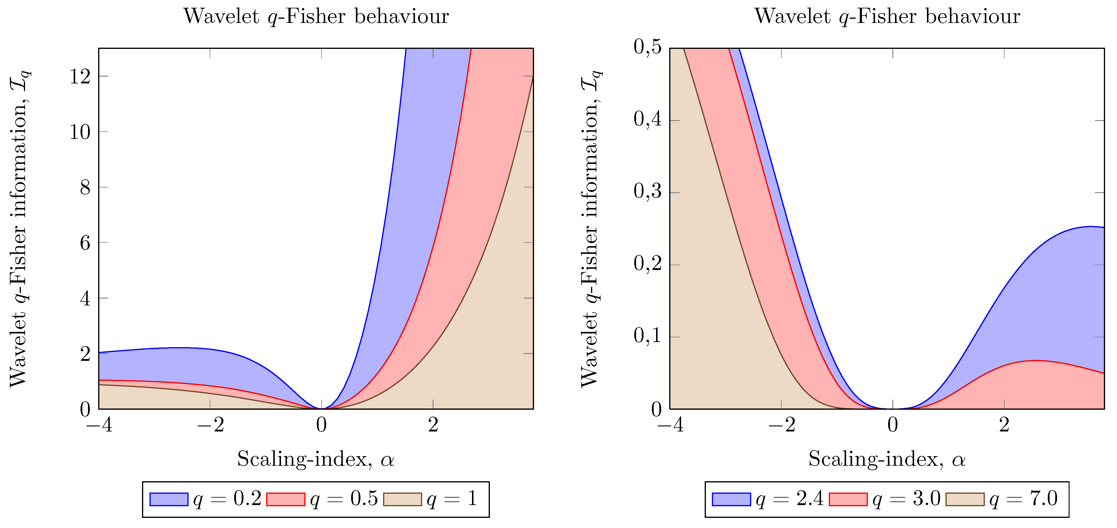
3.2. Wavelet q-Fisher Information

This article defines a generalized version of Fisher information in the wavelet domain (called wavelet q-Fisher information), derives a closed-form expression of this quantifier for scaling signals, and explores the possibility of using wavelet q-Fisher information for the analysis of scaling signals. Let $\{X_t,t\in \mathbb{R}\}$ be a real-valued scaling process satisfying Equation (1), with DWT $\{d_X(j,k),(j,k)\in {\mathbb{Z}}^2\}$ and associated wavelet spectrum $\mathbb{E}|d_X{(j,k)|}^2\sim c_{X_t}{2}^{j\alpha }$ ($c_{X_t}$ a constant and $\mathbb{E}$ the expectation operator) [8]. A pmf obtained from the wavelet spectrum of scaling signals is given by the expression [9,38,39,40,41]

$$p_j\equiv \frac{1/N_j{\sum }_k\mathbb{E}{d}_X^2(j,k)}{{\sum }_{i=1}^M\left\{1/N_i{\sum }_k\mathbb{E}{d}_X^2(i,k)\right\}}=2^{(j-1)\alpha }\frac{1-2^{\alpha }}{1-2^{\alpha M}}$$

(11)

where $N_j$ (respectively $N_i$) represents the number of wavelet coefficients at scale j (respectively i), $M={\text{log}}_2\left(N\right)$ with $N\in {\mathbb{Z}}_{+}$ the length of the data and $j=1,2,\dots ,M$. Substituting Equation (11) into Equation (10) results in the wavelet q-Fisher information of a scaling signal which is given by

$$\begin{array}{ccc}\mathrm{(12)}& \hfill {\mathcal{I}}_q& =& {\left(1-2^{\alpha }\right)}^2{\left\{\frac{1-2^{\alpha }}{1-2^{\alpha M}}\right\}}^q\left\{\frac{1-2^{\alpha q(M-1)}}{1-2^{\alpha q}}\right\}\hfill & =& 2^{\alpha (1-q/2)+2}\left\{{sinh}_{1-v_1}^2\left(u_2\right)\right\}\left\{\frac{{sinh}_{1-v_2/(M-1)}^q\left(u_2\right)}{{sinh}_{1-v_1}\left(u_1\right)}\right\}\hfill \\ \mathrm{(13)}& & \times & \left\{\frac{{sinh}_{1-v_1}\left(u_1\right)}{{sinh}_{1-v_2}^q\left(u_2\right)}\right\}\left\{\frac{P_{\text{num}}}{P_{\text{den}}}\right\}\hfill \end{array}$$

where $P_{\text{num}}$ and $P_{\text{den}}$ are given by the following polynomial expressions

$$\begin{array}{ccc}\hfill P_{\text{num}}& =& 2{cosh}_{1-\frac{v_1}{(M-2)}}\left(u_1(M-2)\right)+2{cosh}_{1-\frac{v_1}{(M-4)}}\left(u_1(M-4)\right)\hfill \\ \mathrm{(14)}& & +& 2{cosh}_{1-\frac{v_1}{(M-6)}}\left(u_1(M-6)\right)+\dots \hfill \end{array}$$

$$\begin{array}{ccc}\hfill P_{\text{den}}& =& 2{cosh}_{1-\frac{v_2}{(M-1)}}\left(u_2(M-1)\right)+2{cosh}_{1-\frac{v_2}{(M-3)}}\left(u_2(M-3)\right)\hfill \\ \mathrm{(15)}& & +& 2{cosh}_{1-\frac{v_2}{(M-5)}}\left(u_2(M-5)\right)+\dots \hfill \end{array}$$

with $u_1=\alpha q{\text{ln}}_q\left(2\right)/2,u_2=q{u}_1,v_1=2(1-q)/\left(\alpha q\right)$ and $v_2=q{v}_1$ Equations (13)–(23) involve the use of the q-analysis [42], where

$${sinh}_q\left(x\right)\equiv \{{\text{e}}_q^x-{\text{e}}_q^{{\ominus }_{q}x}\}/2$$

(16)

$${cosh}_q\left(x\right)\equiv \{{\text{e}}_q^x+{\text{e}}_q^{{\ominus }_{q}x}\}/2$$

(17)

denote the q-sinh and q-cosh functions and

$${\text{e}}_q^x\equiv {\{1+(1-q)x\}}^{1/(1-q)}$$

(18)

$${\ominus }_{q}x\equiv (-x)/\{1+(1-q)x\}$$

(19)

denote the q-exponential and q-difference functions. Equation (13) allows to relate the results of wavelet q-Fisher information with the ones of the standard wavelet Fisher information measure. As a matter of fact, in the $q\to 1$ limiting case, wavelet q-Fisher information turns out to be the standard wavelet Fisher information for which the following holds:

$$I_1=\frac{{\left(2^{\alpha }-1\right)}^2\left(1-2^{\alpha (M-1)}\right)}{1-2^{\alpha M}}$$

(20)

$$=2^{\frac{\alpha }{2}+2}{sinh}^2(\alpha ln2/2).\left\{\frac{P_{num}^M\left(2cosh(\alpha ln2/2)\right)}{P_{den}^{M+1}(2cosh(\alpha ln2/2))}\right\}$$

(21)

where $P_{num}^M(.)$ and $P_{den}^{M+1}(.)$ denote polynomials of argument $2cosh(\alpha ln2/2)$ that are given by

$$\begin{array}{ccc}\hfill P_{num}^M(.)& =& {(2coshu)}^M-\frac{2(M-3)}{2!}{(2coshu)}^{M-2}\hfill \\ \mathrm{(22)}& & +& \frac{3(M-4)(M-5)}{3!}{(2coshu)}^{M-4}-\dots \hfill \end{array}$$

$$\begin{array}{ccc}\hfill P_{den}^{M+1}(.)& =& {(2coshu)}^{M+1}-\frac{(M-2)}{1!}{(2coshu)}^{M-1}\hfill \\ \mathrm{(23)}& & +& \frac{(M-3)(M-4)}{2!}{(2coshu)}^{M-3}-\dots \hfill \end{array}$$

where $u=\alpha ln2/2$. Parameter q provides further analysis flexibility and allows to potentially emphasize some characteristics in the data under study. In [19], the wavelet Fisher’s information was introduced and the wavelet Fisher information plane was presented. An interesting question is how the information plane is affected by the value of the parameter q. Since q is allowed to vary from −∞ to +∞, the present article studies relevant features in some key ranges of q. Figure 2 shows the effect of the parameter q on the information planes obtained by wavelet q-Fisher information, and as a consequence, it is possible to study with some detail the complexities of scaling signals in different ranges of the scaling parameter α.

The wavelet q-Fisher information planes shown in Figure 2 display the Fisher information (in wavelet domain) for $q\in (0,1)$ for various stationary and nonstationary scaling processes. Note that as $q\to 0$, the wavelet q-Fisher information of nonstationary signals ($\alpha >0$) increases exponentially. Nonstationary signals are therefore more perceptible or attain high Fisher’s information (when $q\to 0$) than stationary scaling signals. Note that as long as $q\in (0,1)$, the form of the wavelet q-Fisher information planes are similar in shape. This shape is preserved as long as $q<2$. For the special case $q>2$, a completely different behaviour is observed on Fisher planes. Also note that as long as $q\in (0,1)$, the stationary scaling signals Fisher information are small. Figure 3 displays the wavelet q-Fisher information plane for scaling signals when $q\ge 2$. When $q=2$, wavelet q-Fisher information is symmetrical around $\alpha =0$ and the Fisher information observed at the right of $q=2$ are identical to those observed at the left of that point. For $q=3$, wavelet q-Fisher information is high for stationary signals and low for nonstationary ones. Note that this behaviour is contrary (opposite) to the behaviour observed for this quantifier when $q\in (0,1)$. Based on this, wavelet q-Fisher information reverses its behaviour as long as $q>2$. The boundary $q=2$, therefore, permits wavelet q-Fisher information to highlight nonstationary or stationary phenomena (or processes). For $q\to \infty$, nonstationary phenomena is zero. Figure 4 reviews the behavior observed in the wavelet q-Fisher information planes for $q<2$ and $q\ge 2$.

Figure 2. Wavelet q-Fisher information for $1/f^{\alpha }$ signals. Top left plot displays the Fisher information with $q=0.2$, top right with $q=0.4$. Bottom left graph represents Fisher information for $q=0.6$ and bottom right plot with $q=0.8$.

Figure 2. Wavelet q-Fisher information for $1/f^{\alpha }$ signals. Top left plot displays the Fisher information with $q=0.2$, top right with $q=0.4$. Bottom left graph represents Fisher information for $q=0.6$ and bottom right plot with $q=0.8$.

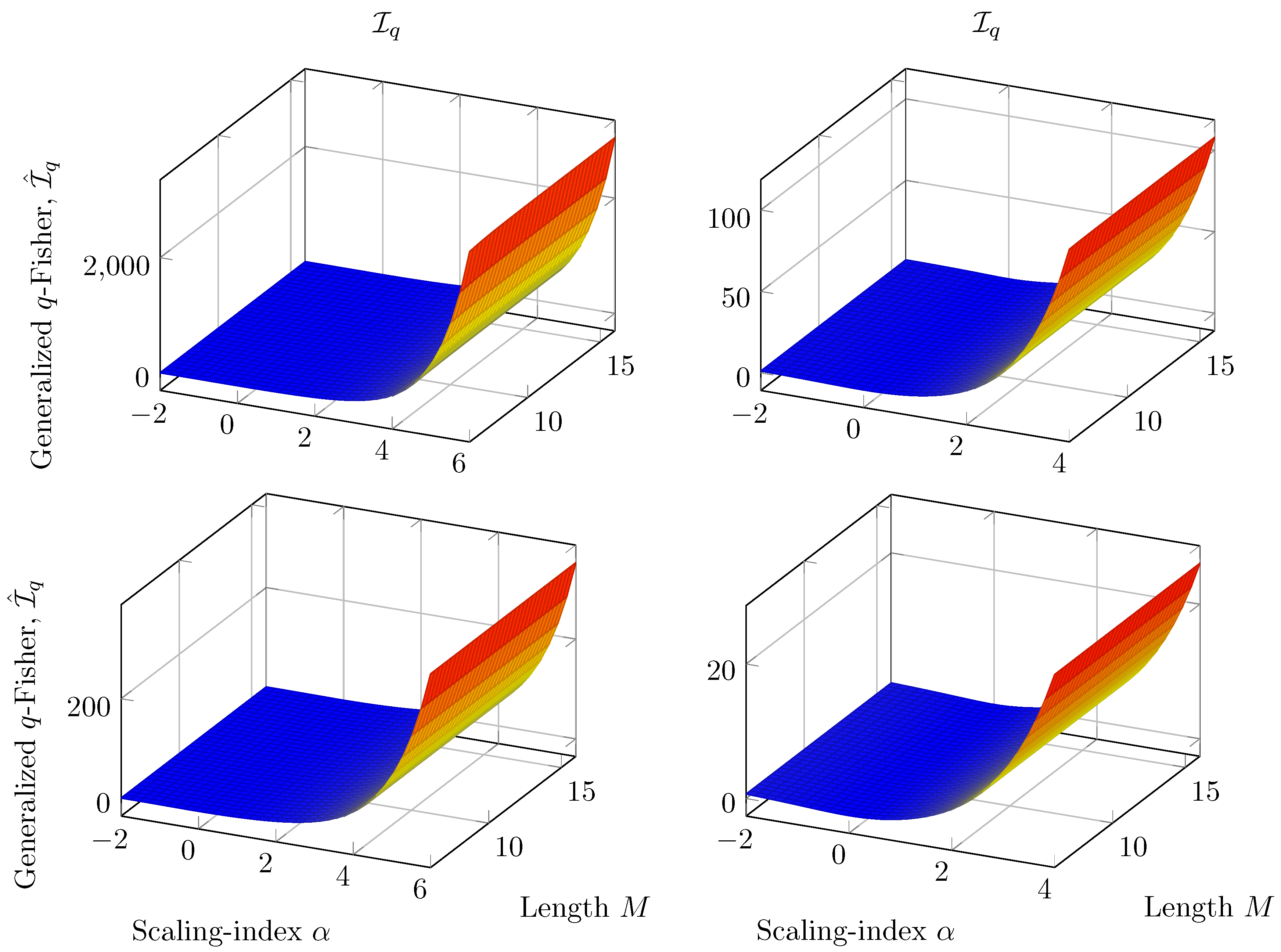
3.3. Applications of Wavelet Fisher’s Information Measure

As studied above, wavelet q-Fisher information allows to discern between stationary and nonstationary scaling signals, which equivalently, allows to suitably describe the complexities within these signals. Based on the fact that wavelet q-Fisher information has large values for non-stationary signals and small values for stationary ones (for the case $q\in (0,1)$), a potential application area of wavelet q-Fisher information is in the classification of fractal signals as fractional noises and motions. Classification of $1/f^{\alpha }$ signals as motions or noises remains as an important, attractive and unresolved problem in scaling signal analysis [10,43,44] since the nature of the signal governs the selection of estimators, the shape of quantifiers such as $qth$ order moments, the nature of correlation functions, etc. [45]. The correct classification of scaling signals avoids many estimation issues, however, it is not trivial in the limit of $\alpha \to 1$. Another important potential application of wavelet q-Fisher information, related to the classification of signals, is in the blind estimation of scaling parameters [46]. Blind estimation refers to estimating α, independently of signal type (stationary or non-stationary). Wavelet q-Fisher information can also be utilized for the detection of structural breaks in the mean embedded in $1/f^{\alpha }$ signals. Structural breaks in the mean affect significantly the estimation of scaling parameters leading to biased estimates of the parameter α and consequently in misinterpretation of the phenomena.

Figure 3. Wavelet q-Fisher information for $1/f^{\alpha }$ signals. Top left plot displays the Fisher information with $q=2.5$, top right with $q=3$. Bottom left graph represents Fisher information for $q=3.5$ and bottom right plot with $q=4$.

Figure 3. Wavelet q-Fisher information for $1/f^{\alpha }$ signals. Top left plot displays the Fisher information with $q=2.5$, top right with $q=3$. Bottom left graph represents Fisher information for $q=3.5$ and bottom right plot with $q=4$.

Stoev and coworkers [8] demonstrated that the well-known Abry–Veitch estimator [27,28] overestimates the scaling index α in the presence of a single level-shift which gives rise to values of $H=(\alpha +1)/2>1$, which in principle are not permissible in the theory of self-similar signals. In the following, the paper concentrates on the detection of structural breaks in the mean embedded in synthesized stationary fGn signals by the use of wavelet q-Fisher information. Figure 5 illustrates a flowchart that can be used for enhancing the estimation of the scaling parameter α for scaling signals with multiple structural changes. The first step is to detect and locate structural changes followed by the quantification of the amplitude of the structural changes and the elimination of the structural changes in the signal.

Figure 4. Wavelet q-Fisher information of scaling signals. Wavelet q-Fisher information is exponentially increasing (or decreasing) for signals with $\alpha >0$ (or $-\infty <\alpha <0$) and minimum for scaling signals with $\alpha =0$.

Figure 4. Wavelet q-Fisher information of scaling signals. Wavelet q-Fisher information is exponentially increasing (or decreasing) for signals with $\alpha >0$ (or $-\infty <\alpha <0$) and minimum for scaling signals with $\alpha =0$.

Figure 5. Estimation of the scaling index α in the presence of structural changes in the mean. The estimation involves three steps, level-shift detection & location, level-shift quantification & elimination and estimation of the scaling index in a time series with no structural changes.

Figure 5. Estimation of the scaling index α in the presence of structural changes in the mean. The estimation involves three steps, level-shift detection & location, level-shift quantification & elimination and estimation of the scaling index in a time series with no structural changes.

The final step is to estimate the scaling parameter α with some standard method of estimation such as the Abry–Veitch estimator. Without the use of this methodology, significant biases in the estimation of α can be obtained, which in turn gives rise to misinterpretation of the phenomena under study. This article studies anti-correlated and correlated versions of fractional Gaussian noises and the power of wavelet q-Fisher information in detecting single structural breaks in the mean within these signals.

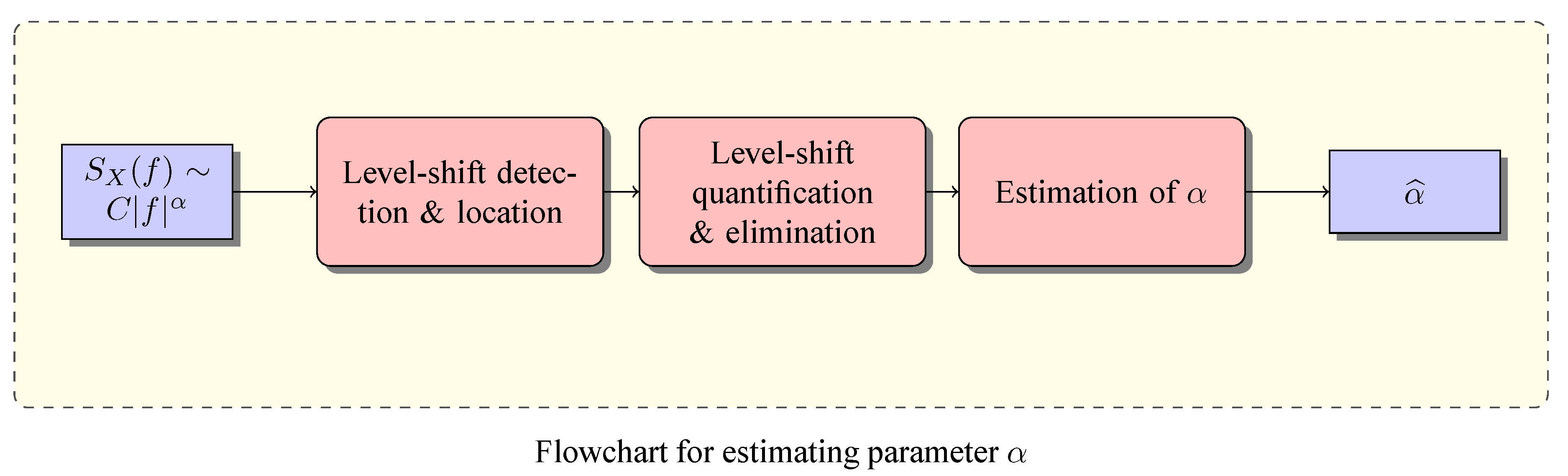
4. Level-Shift Detection Using Wavelet q-Fisher Information

4.1. The Problem of Level-Shift Detection

Detection and location of structural breaks in the mean (level-shifts) has been recognized as an important research problem in many areas of science [47,48]. In the Internet traffic analysis framework, detection, location and mitigation of level-shifts significantly improves on the estimation process. Moreover, it has been demonstrated [8] that the presence of a single level-shift embedded in a stationary fGn will result in an estimated $H>1$ [8] (estimated using wavelet-based methodologies). This is turn results in misinterpretation of the phenomena under study, inadequate construction of $qth$-order moments, etc. Let $B\left(t\right),t\in \mathbb{R}$ be a $1/f$ signal with level-shifts at time instants $\{t_1,t_{1+L},\dots t_j,t_{j+L}\}$. $B\left(t\right)$ can be represented as

$$B\left(t\right)=X\left(t\right)+\sum _{j=1}^J{\mu }_j{\mathbf{1}}_{[t_j,t_{j+L}]}\left(t\right)$$

(24)

where $X\left(t\right)$ is a signal satisfying Equation (1) and ${\mu }_j{\mathbf{1}}_{[a,b]}\left(t\right)$ represents the indicator function of amplitude ${\mu }_j$ in the interval $[a,b]$. The problem of level-shift detection reduces to identify the points ${\{t_j,t_{j+L}\}}_{j\in J}$ where a change in behaviour occurs. Often, the change is perceptible by eye, but frequently this is not the case and alternative quantitative methods are preferred. In what follows, a description of the procedure for detecting level-shifts in $1/f$ signals by wavelet q-Fisher information is described and later results on simulated fGn and H$.263$ encoded video signals are presented.

4.2. Level-Shift Detection Using Wavelet q-Fisher Information

To detect the presence of level-shifts in fractal $1/f$ signals, wavelet q-Fisher information is computed in sliding windows. A window of length W, located in the interval $m\Delta \le t_k<m\Delta +W$ applied to signal $\{X\left(t_k\right),k=1,2,\dots N\}$ is

$$X(m;W,\Delta )=X\left(t_k\right)\Pi \left(\frac{t-m\Delta }{W}-\frac{1}{2}\right)$$

(25)

where $m=0,1,2,\dots m_{max}$, Δ is the sliding factor and $\Pi (.)$ is the well-known rectangular function. Note that Equation (25) represents a subset of $X\left(t_k\right)$ and thus by varying m from 0 to $m_{max}$ and computing wavelet q-Fisher’s information on every window, the temporal evolution of wavelet q-Fisher information is followed. Suppose the wavelet q-Fisher information at time m (for sliding factor Δ) is denoted as ${\mathcal{I}}_X\left(m\right)$, then a plot of the points

$${\left\{\left(W+m\Delta ,{\mathcal{I}}_X\left(m\right)\right)\right\}}_{m=0}^{m_{max}}:={\mathcal{I}}_q$$

(26)

represents such time-evolution. In [8], it was demonstrated that the presence of a sudden jump in a stationary fractal signal will cause the estimated $\widehat{H}>1$. The level-shift, thus, causes the signal under observation to become non-stationary. In the wavelet Fisher’s information framework, this sudden jump will cause its value to increase suddenly. Therefore a sudden jump increase (in the form of an impulse) in the plot of Equation (26) can be considered as an indicator of the occurrence of a single level-shift in the signal. These theoretical findings are experimentally tested by the use of synthesized scaling signal with level-shifts. The synthesized signals correspond to fGn signals generated using the circular embedding algorithm [49,50] (also known as the Davies and Harte algorithm).

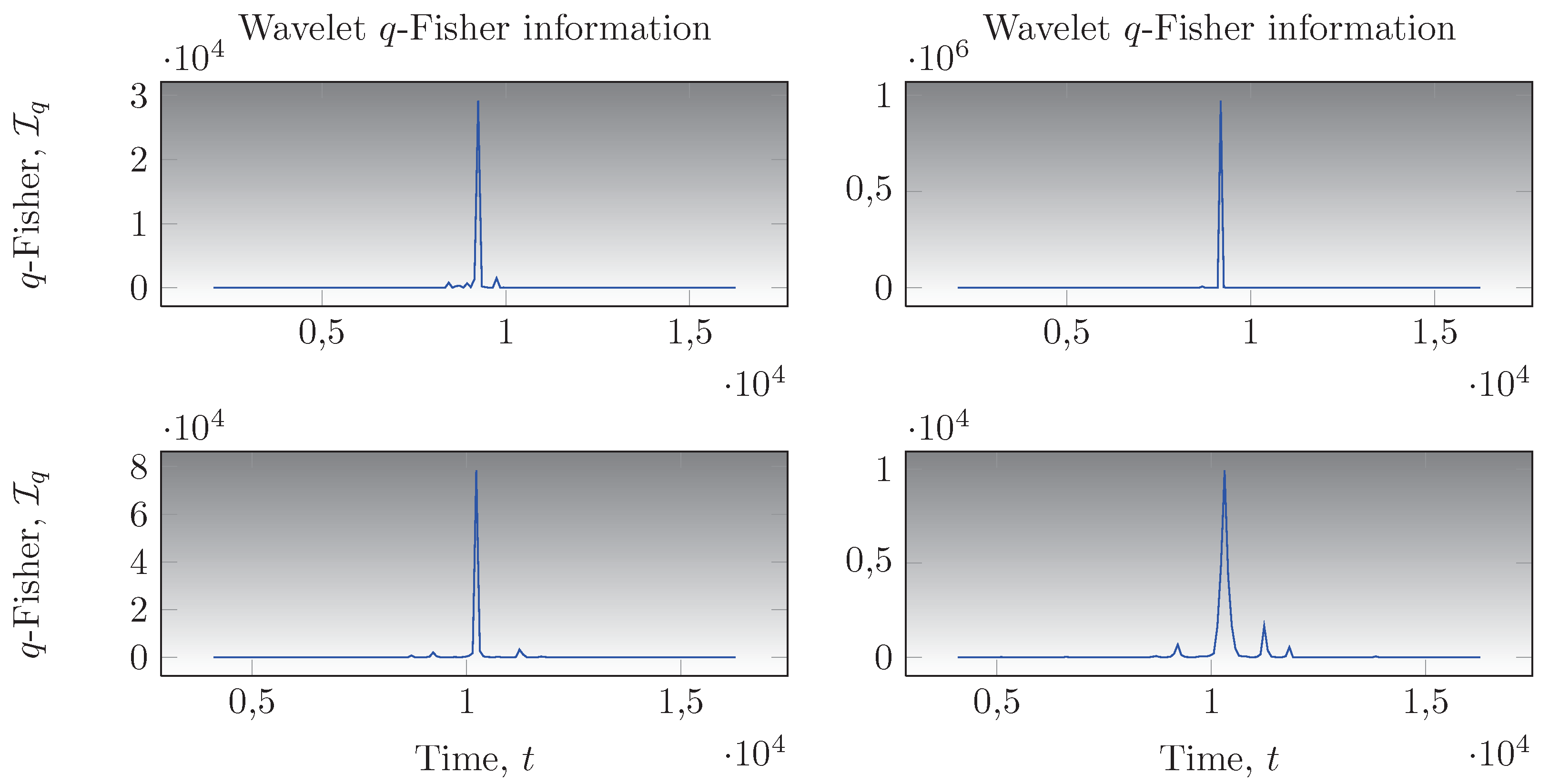
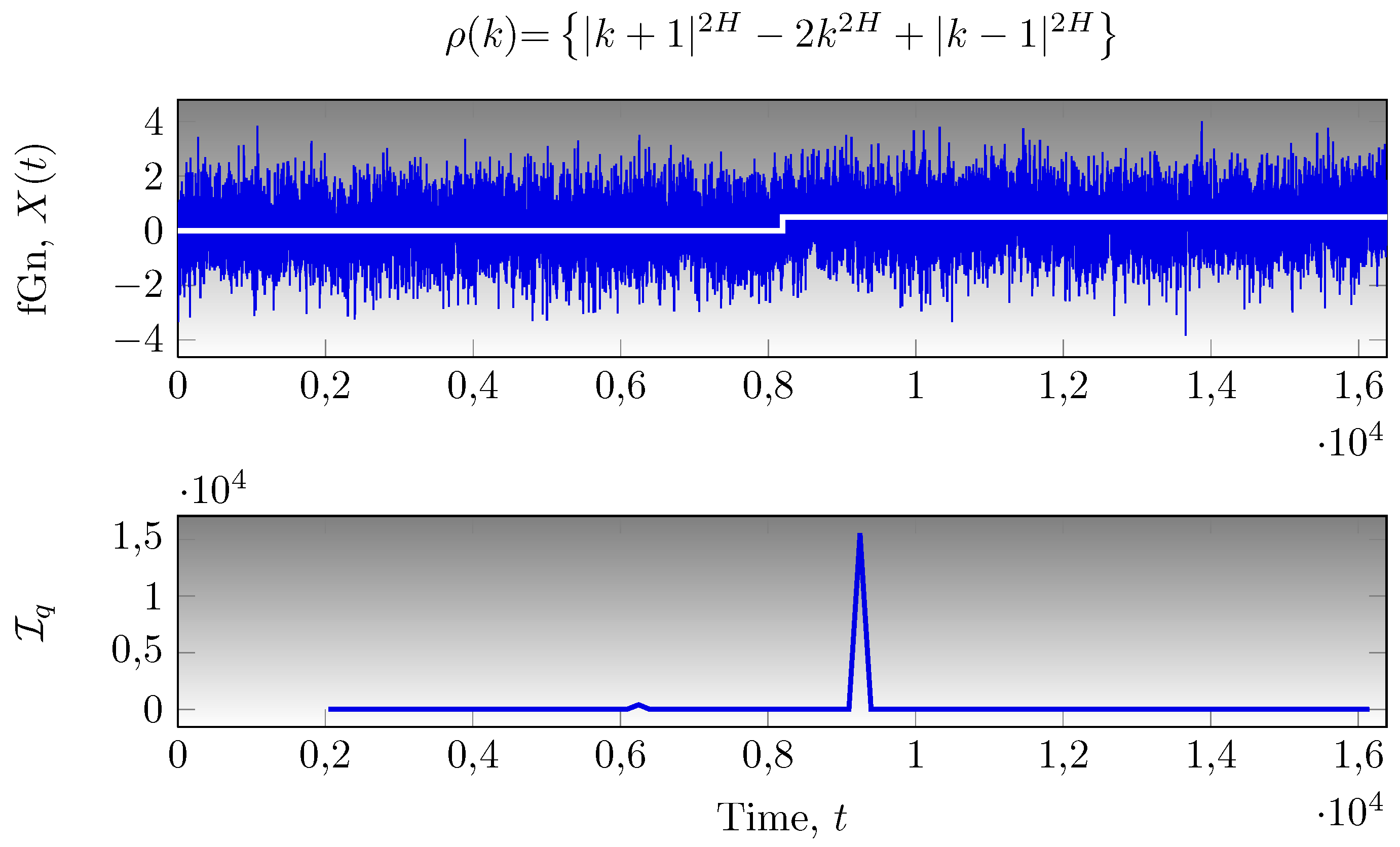
5. Results and Discussion

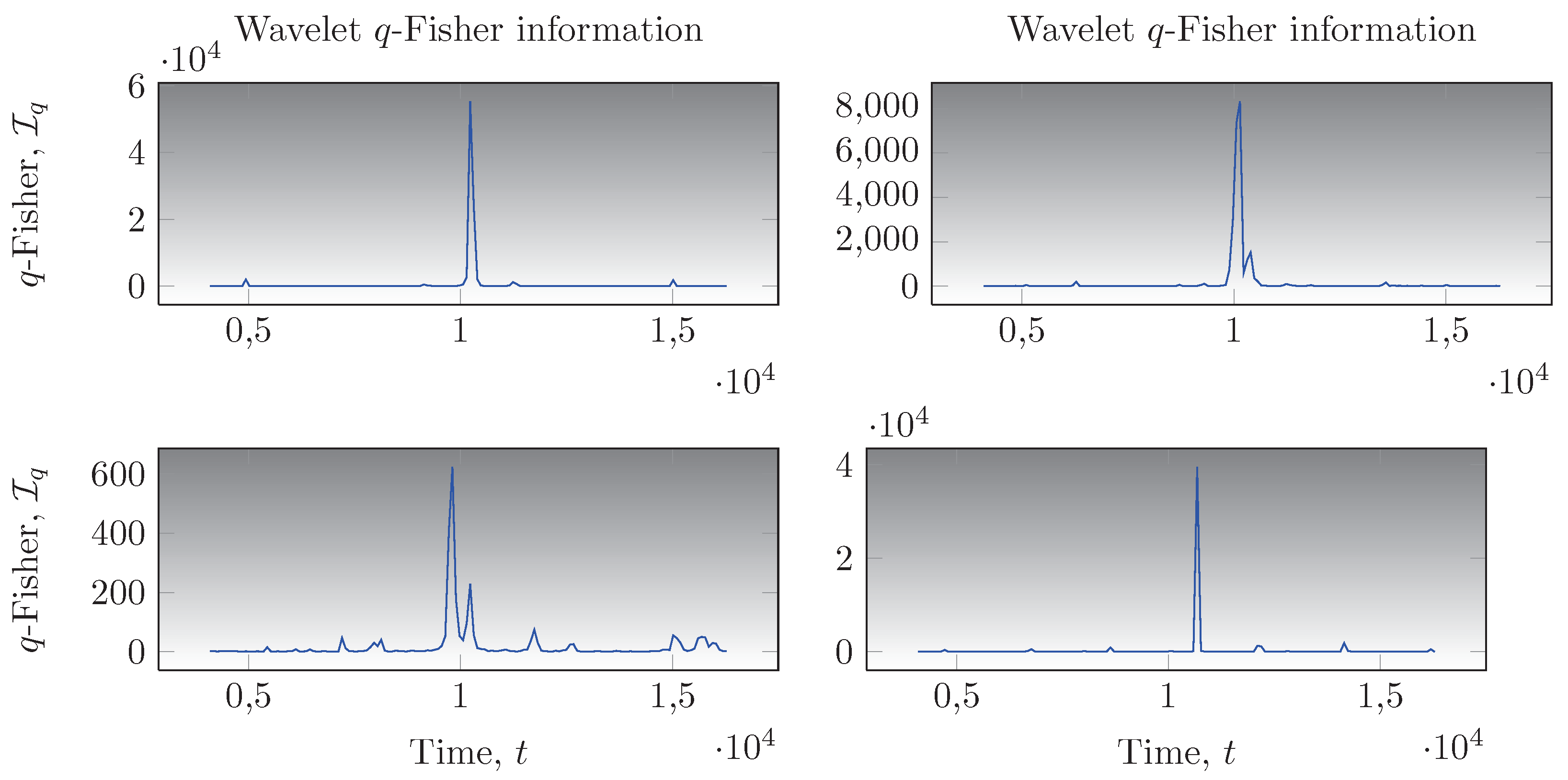
5.1. Analysis of fGn Signals with Single Level-Shifts

Figure 6 displays the level-shift detection capabilities of wavelet q-Fisher information for a self-similar, long-memory fGn with Hurst exponent $H=0.7$ and a single structural break embedded within its structure.

Figure 6. Detection of a single structural break at $t_b=8192$ embedded in a fractional Gaussian noise signal with parameter $H=0.7$.

Figure 6. Detection of a single structural break at $t_b=8192$ embedded in a fractional Gaussian noise signal with parameter $H=0.7$.

The structural break is located at $t_b=8192$, i.e., in the middle of the time series. The amplitude of the level-shift is $\sqrt{{\sigma }_X^2}/2$, where ${\sigma }_X^2$ is the variance of the analyzed fGn signal. Top plot displays the graph of a stationary fGn signal with a single level-shift. For illustration purposes, the level-shift is also shown in white within this figure. Note that the level-shift embedded within the fGn is imperceptible, therefore, its detection becomes complex. Many articles in the literature claim that a given technique is a good level-shift detection tool, however, they present results on solely anticorrelated signals with large level-shifts. As stated above, an impulse-like peak in the wavelet q-Fisher plot is an indicator of a level-shift in the analyzed signal. Note from bottom plot of Figure 6 that wavelet q-Fisher information not only detects the weak level-shift but also locates it with reasonable accuracy. Level-shifts with amplitudes greater than $\sqrt{{\sigma }_X^2}/2$ are also efficiently detected by wavelet q-Fisher information. The results presented in bottom plot of Figure 6 were computed using a value of $q=0.6$. In order to efficiently detect weak level-shifts embedded in correlated fGn signals, the value of q must lie within $(0,1)$; the more correlated the signal (and also the more weaker the level-shift) the lower the value of q. Decreasing the value of q has the effect of increasing the amplitude of the impulse-shaped peak in the wavelet q-Fisher information which in consequence makes the detection easier. Multiple weak level-shifts are also efficiently detected by wavelet q-Fisher information. As wavelet q-Fisher information is computed in sliding windows, multiple weak level-shifts are not only detected but also located. The more correlated the signal, the more difficult it is to detect and locate the level-shifts. Figure 7 displays the wavelet q-Fisher information for anticorrelated fGn signals with a single level-shift.

Figure 7. Wavelet q-Fisher information for anticorrelated fGn signals. Top left plot displays the wavelet q-Fisher information for a fGn signal with $H=0.1$, top right plot with $H=0.2$, bottom left plot for $H=0.3$ and finally bottom right plot for $H=0.4$. The amplitude of level-shifts was set to $\sqrt{{\sigma }_X^2}/2$.

Figure 7. Wavelet q-Fisher information for anticorrelated fGn signals. Top left plot displays the wavelet q-Fisher information for a fGn signal with $H=0.1$, top right plot with $H=0.2$, bottom left plot for $H=0.3$ and finally bottom right plot for $H=0.4$. The amplitude of level-shifts was set to $\sqrt{{\sigma }_X^2}/2$.

The level-shift amplitude is $\sqrt{{\sigma }_X^2}/2$ and is located in the middle of the time series with length $N=2^{14}$. Top left plot displays the wavelet q-Fisher information for a fGn signal with Hurst exponent $H=0.1$. Note that a large impulse-shaped peak indicates the presence of a single level-shift embedded in the fGn signal under study. The wavelet q-Fisher information was computed in sliding windows with window-length $W=2^{11}$ at sliding factor of $\Delta =90$. Parameter q was set to $q=0.6$. Top right plot displays the Fisher information of a fGn signal (with $H=0.2$) with a single level-shift. Note that the presence of the level-shift is shown by the large impulsive peak in the wavelet q-Fisher information plot. Bottom plots display the wavelet q-Fisher information for fGn signals with $H=0.3$ and $H=0.4$. Wavelet q-Fisher information plot detects, as in the previous cases, the presence of the single level-shift by an impulse shaped peak in the middle of the time series. Similar results are obtained when analyzing anti-correlated fGn with $H<0.5$, which in principle indicates that wavelet q-Fisher information detects the presence of a single weak level-shift embedded in anticorrelated self-similar signals. Recall that anti-correlated signals share the property that large values are likely to be followed by low values, or equivalently, positive values are likely to be followed by negative values. Figure 8 displays the wavelet q-Fisher information plots for long-memory, self-similar fGn signals.

Figure 8. Wavelet q-Fisher information for Gaussian white noise and correlated fGn signals. Top left plot displays the wavelet q-Fisher information for a Gaussian white noise signal ($H=0.5$), top right plot for a fGn signal with $H=0.6$, bottom left plot for a fGn signal with $H=0.8$ and finally bottom right plot for a fGn with $H=0.9$. The amplitude of level-shifts was set to $\sqrt{{\sigma }_X^2}/2$.

Figure 8. Wavelet q-Fisher information for Gaussian white noise and correlated fGn signals. Top left plot displays the wavelet q-Fisher information for a Gaussian white noise signal ($H=0.5$), top right plot for a fGn signal with $H=0.6$, bottom left plot for a fGn signal with $H=0.8$ and finally bottom right plot for a fGn with $H=0.9$. The amplitude of level-shifts was set to $\sqrt{{\sigma }_X^2}/2$.

Top left plot displays the wavelet q-Fisher information for a random Gaussian white noise (fGn with $H=0.5$). As in the previous analyses, wavelet q-Fisher information is computed using $q=0.6$ and sliding windows with $W=2^{11}$ and $\Delta =90$. This and the previous results indicate that wavelet q-Fisher information detects the presence of level-shifts embedded in fGn signals which are either anticorrelated or completely random, i.e., level-shifts are detected as long as the Hurst parameter in fGn signals is $H\le 5$. The rest of the plots of Figure 8 display the level-shift detection capabilities of wavelet q-Fisher information for correlated fGn signal. The stationarity and self-similarity conditions are still satisfied and the correlation within observations varied. Top right plot displays the wavelet q-Fisher information for a fGn signal with weak long-memory ($H=0.6$) and a single level-shift (with amplitude $\sqrt{{\sigma }_X^2}/2$). The level-shift within the signal is correctly detected by wavelet q-Fisher information. Bottom left and bottom right plots of Figure 8 display the wavelet q-Fisher information for strongly correlated ($H=0.8$ and $H=0.9$ respectively) stationary fGn signals with a single level-shift within its structure. Note that in both plots the level-shifts are correctly detected by wavelet q-Fisher information and for the case of single level-shifts, wavelet q-Fisher information detects effectively these nonstationarities for anti-correlated, random and correlated stationary fGn signals.

5.2. Comparison with Other Methods

Wavelet q-Fisher information not only detects but also, with some accuracy, locates single and multiple level-shifts embedded in fGn signals of parameter H. To test the accuracy of wavelet q-Fisher information as a structural break detection and location technique, a comparative study with some standard methodology of breakpoint location is performed using synthesized fGn signals. Anticorrelated and correlated fGn signals are used to test how well wavelet q-Fisher’s information (along with some breakpoint detection/location technique) locates single structural breaks embedded in the middle of the process. The well-known Bai & Perron algorithm [20] for multiple structural change detection is used in this article. The Bai & Perron algorithm is tested against a reduced size time series of wavelet q-Fisher information for which the same Bai & Perron algorithm is applied. Thus, the Bai & Perron algorithm is used along with wavelet q-Fisher information in order to date the structural change detected by wavelet q-Fisher information. The advantage of using the Bai & Perron algorithm in wavelet q-Fisher information time series is that it is possible to investigate the presence of multiple structural changes in long traces in a fraction of the time required in the standard Bai & Perron algorithm.

Table 2. Comparison of wavelet q-Fisher information based Bai & Perron technique for breakpoint detection with Bai & Perron algorithm. The traces used were synthesized using the fGn model with length $N=4096$ and a single break at $t_b=2048$.

Statistics	Breakpoint detection using fGn signals
	Nominal H
	Bai & Perron algorithm			Wavelet FIM Bai & Perron
	0.3	0.5	0.7	0.3	0.5	0.7
BIAS	$-0.53$	$-0.83$	456.1	$-464.6$	$-490$	$-439$
σ	4.41	32.2	569	138	256	562
$\sqrt{\text{MSE}}$	4.37	31.64	722.33	484.1	551.1	706.4
μ	2048	2048	1591	2512	2538	2487
$\text{min}\left(\right)$	2040	2000	646	2184	2104	1444
$\text{max}\left(\right)$	2058	2186	2159	2844	3624	3624

Table 2. Comparison of wavelet q-Fisher information based Bai & Perron technique for breakpoint detection with Bai & Perron algorithm. The traces used were synthesized using the fGn model with length $N=4096$ and a single break at $t_b=2048$.

Statistics	Breakpoint detection using fGn signals
	Nominal H
	Bai & Perron algorithm			Wavelet FIM Bai & Perron
	0.3	0.5	0.7	0.3	0.5	0.7
BIAS	$-0.53$	$-0.83$	456.1	$-464.6$	$-490$	$-439$
σ	4.41	32.2	569	138	256	562
$\sqrt{\text{MSE}}$	4.37	31.64	722.33	484.1	551.1	706.4
μ	2048	2048	1591	2512	2538	2487
$\text{min}\left(\right)$	2040	2000	646	2184	2104	1444
$\text{max}\left(\right)$	2058	2186	2159	2844	3624	3624

For instance, the Bai & Perron algorithm analyzes a trace of $N=4096$ points in almost 10 minutes, while for the wavelet FIM based Bai & Perron algorithm it is performed in seconds. Table 2 presents a comparison of the standard Bai & Perron methodology for structural change detection and location against the same technique using pre-processed (using wavelet q-Fisher information) time series. The techniques were tested using 30 time series of fGn type with Hurst exponents $H=\{0.3,0.5,0,7\}$. The statistics were computed as $\text{BIAS}=\widehat{{\tau }_b}-{\tau }_0$, where ${\tau }_0$ is the location of the structural break and $\widehat{{\tau }_b}$ is the mean structural break dated with some technique. The rest of the statistics are the mean, $\mu =\widehat{{\tau }_b}$, the standard deviation, σ, the min, max and the $\sqrt{MSE}=1/L{\sum }_{j=1}^L{(\widehat{{\tau }_b^j}-{\tau }_0)}^2$. Note from the Table 2 that wavelet q-Fisher information has a BIAS of around $\sim 450$, this BIAS can be explained by the fact that wavelet q-Fisher information detects level-shifts by the presence of a phased impulse-shaped peak. The $\sqrt{MSE}$ values for the wavelet q-Fisher information can also be explained by this phased nature of the peaks within wavelet q-Fisher information. Note that when applied to correlated fGn signals, the wavelet FIM based Bai & Perron algorithm performs better than the standard Bai & Perron algorithm. These results indicate that wavelet FIM based Bai & Perron technique works reasonably well for detecting and locating weak structural changes in fGn signals and that can be applied to long traces since it is fast and robust.

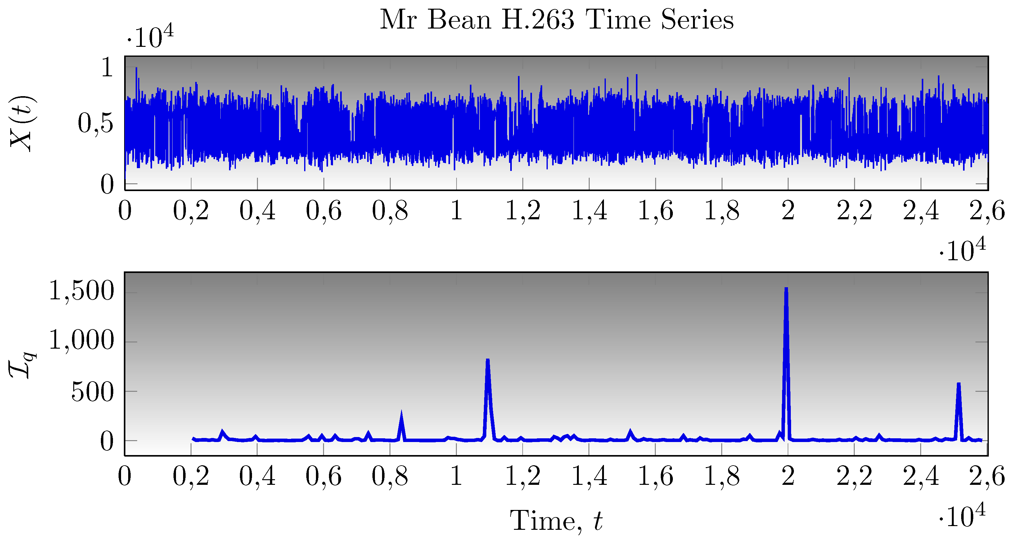
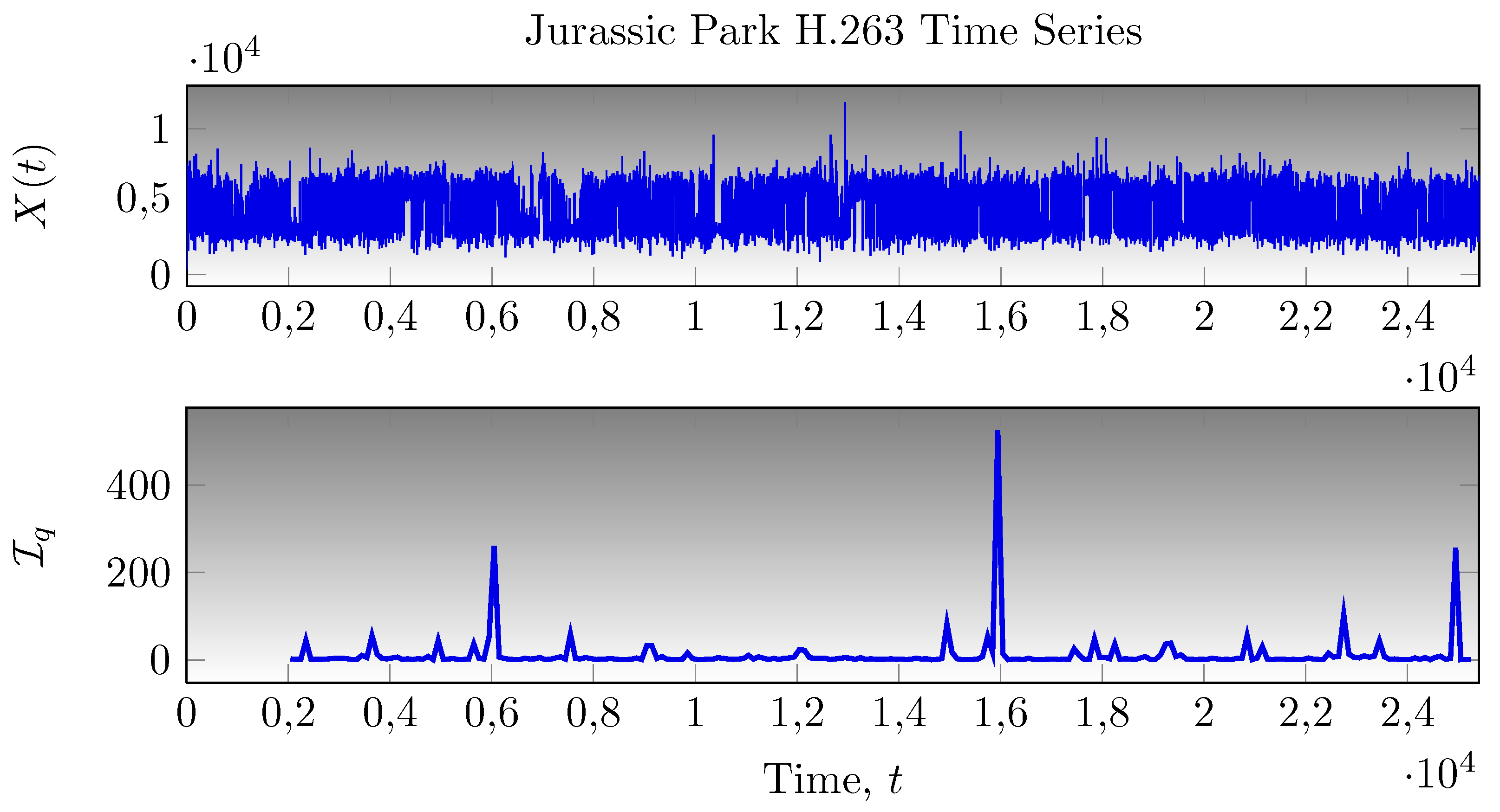
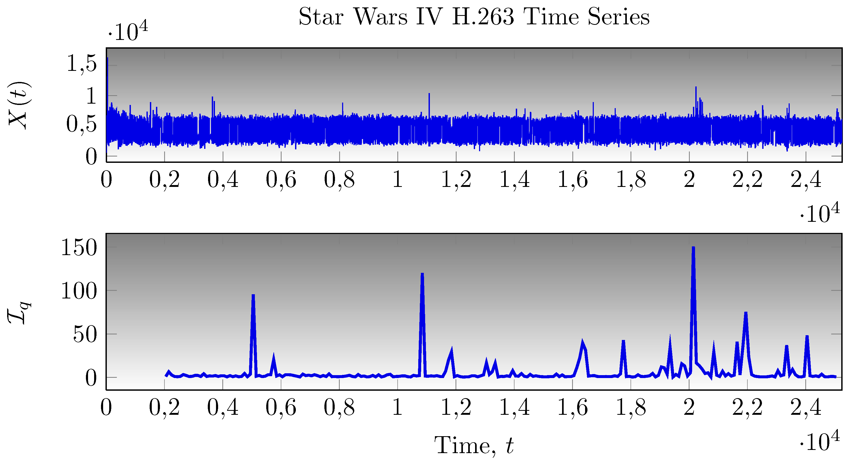
5.3. Application to H.263 Video Traces

H.263 video encoded traffic, along with MPEG-4 video traffic, is expected to account for a large amount of the traffic in both future wireline and wireless computer communications networks [6]. Video traffic is recognized in the literature to possess long-memory characteristics independently of the encoding algorithm used to generate the video trace [5]. Reported statistical studies, for some video traces, indicate the presence of nonstationarities within the traces due to the Hurst parameter estimation $H>1$ and a test for time constancy of the scaling exponent α indicates that the Hurst parameter varies with time. As reported in the work of Stoev [8], a Hurst parameter estimation greater than 1 indicates the presence of a level-shift embedded in the time series under study. A single level-shift in a fGn time series causes the estimated Hurst parameter within the signal (using wavelet based estimation) to be greater than 1. In this section, we explore the wavelet q-Fisher information for some publicly available video traces and discuss the stationarity nature of the video traces based on the estimated wavelet Fisher information. The traces studied were obtained at Technical University of Berlin web page and represent 60 minutes of H.263 video encoded traffic using 256 kbit/s target bit rate. Top plot of Figure 9 displays the time series of H.263 encoded Mr. Bean movie. Each point of the time series represents the number of bits of each frame size. The total length of the encoded Mr. Bean movie is $26,034$ points. The Hurst parameter of Mr. Bean movie is $H>1$, which indicates the presence of some nonstationarity within the signal. Bottom plot of Figure 9 display the wavelet q-Fisher information (with $q=0.8$) of Mr. Bean movie computed in sliding windows of length $W=2048$ and sliding factor of $\Delta =100$. Note that the wavelet q-Fisher information of Mr. Bean movie displays some impulse-shaped peaks at $t\sim \{8000,11000,20000,25000\}$ which according to the previous discussion on simulated signals indicate the presence of level-shifts embedded in the time series under study. The presence of peaks within a signal indicates in consequence that different regions of similar behavior are observed within the signal. This is turn indicates that current stationary models for video sequences need to be revised thoroughly. Similar behavior of the wavelet q-Fisher information is observed when varying the parameter q in the interval $q\in (0,1)$. By approaching $q\to 0$, some level-shifts in the form of impulses are amplified. The results of the wavelet q-Fisher information are similar as those presented in [6] in the sense that the presence of peaks indicate that the scaling exponents are not constant in time and that the presence of level-shifts causes the estimated Hurst parameter $H>1$.

Figure 10 displays the time series obtained by encoding the Jurassic Park movie with H.263 algorithm and the wavelet q-Fisher information of the encoded video trace. The length of the time series is $25,407$ points and the wavelet q-Fisher information was computed with $q=0.8$, $W=2048$ and $\Delta =100$.

Note from the bottom plot of Figure 10 that the wavelet q-Fisher information of Jurassic Park movie presents, as in the previous case, several impulse-shaped peaks indicating the presence of level-shifts within the encoded video signal. Finally Figure 11 displays the encoded video signal of Star Wars IV movie along with the wavelet q-Fisher information of this signal computed with $q=0.8$, $W=2048$ and $\Delta =100$. The length of this H.263 encoded video signal is $25,243$. Note that as in the previous analyses, impulse shaped peaks are found in the wavelet q-Fisher information of this signal. These results indicate that H.263 encoded video signals display nonstationary features which need to be taken into account since future wireline and wireless networks will likely support this type of traffic.

Figure 9. Wavelet q-Fisher information for an H.263 encoded video signal. Top plot displays the time series (frame size in bits) of Mr. Bean movie and bottom plot shows the wavelet q-Fisher information of Mr. Bean movie using a $q=0.8$.

Figure 9. Wavelet q-Fisher information for an H.263 encoded video signal. Top plot displays the time series (frame size in bits) of Mr. Bean movie and bottom plot shows the wavelet q-Fisher information of Mr. Bean movie using a $q=0.8$.

Figure 10. Wavelet q-Fisher information for an H.263 encoded video signal. Top plot displays the time series (frame size in bits) of Jurassic Park movie and bottom plot shows the wavelet q-Fisher information of Jurassic Park movie using a $q=0.8$.

Figure 10. Wavelet q-Fisher information for an H.263 encoded video signal. Top plot displays the time series (frame size in bits) of Jurassic Park movie and bottom plot shows the wavelet q-Fisher information of Jurassic Park movie using a $q=0.8$.

Figure 11. Wavelet q-Fisher information for an H.263 encoded video signal. Top plot displays the time series (frame size in bits) of Star Wars IV movie and bottom plot shows the wavelet q-Fisher information of Star Wars IV movie using a $q=0.8$.

Figure 11. Wavelet q-Fisher information for an H.263 encoded video signal. Top plot displays the time series (frame size in bits) of Star Wars IV movie and bottom plot shows the wavelet q-Fisher information of Star Wars IV movie using a $q=0.8$.

6. Conclusions

In this article, the definition of wavelet q-Fisher information was presented and the properties of this quantifier for scaling or $1/f^{\alpha }$ processes studied. A closed-form expression of wavelet q-Fisher information was derived for scaling signals in terms of the q-analysis and it was demonstrated that in the $q\to 1$ limit, it converged to the standard wavelet Fisher information. Wavelet q-Fisher information provides further analysis flexibility since q can be adjusted according to the properties and characteristics of the data. For $q>2$, wavelet q-Fisher information reverses its behavior and when $q\in (0,1)$ it can be used for the detection of level-shifts embedded in scaling signals. Experimental studies using synthesized fGn signals and the Bai & Perron algorithm demonstrate that wavelet q-Fisher information not only detects but also locates weak level-shifts embedded within these signals. The application of wavelet q-Fisher information to H.263 encoded video signals was also presented.

References

1. Leland, W.E.; Taqqu, M.S.; Willinger, W.; Wilson, D. On the self-similar nature of ethernet traffic (extended version). IEEE/ACM Trans. Netw. 1994, 2, 1–15. [Google Scholar] [CrossRef]
2. Paxson, V.; Floyd, S. Wide area traffic: The failure of poisson modeling. IEEE/ACM Trans. Netw. 1995, 3, 226–244. [Google Scholar] [CrossRef]
3. Lee, I.W.C.; Fapojuwo, A.O. Stochastic processes for computer network traffic modelling. Comput. Commun. 2005, 29, 1–23. [Google Scholar] [CrossRef]
4. Beran, J. Statistical methods for data with long-range dependence. Stat. Sci. 1992, 7, 404–416. [Google Scholar] [CrossRef]
5. Beran, J.; Sherman, R.; Taqqu, M.S.; Willinger, W. Long-range dependence in variable-bit-rate video traffic. IEEE Trans. Commun. 1995, 43, 1566–1579. [Google Scholar] [CrossRef]
6. Fitzek, F.H.P.; Reisslein, M. MPEG-4 and H.263 video traces for network performance evaluation. IEEE Netw. 2001, 15, 40–54. [Google Scholar] [CrossRef]
7. Shen, H.; Zhu, Z.; Lee, T. Robust estimation of the self-similarity parameter in network traffic using the wavelet transform. Signal Process. 2007, 87, 2111–2124. [Google Scholar] [CrossRef]
8. Stoev, S.; Taqqu, M.S.; Park, C.; Marron, J.S. On the wavelet spectrum diagnostic for Hurst parameter estimation in the analysis of internet traffic. Comput. Netw. 2005, 48, 423–445. [Google Scholar]
9. Ramirez-Pacheco, J.; Torres-Roman, D. Cosh window behaviour of wavelet Tsallis q-entropies in 1 / f α signals. Electron. Lett. 2011, 47, 186–187. [Google Scholar] [CrossRef]
10. Eke, A.; Hermán, P.; Bassingthwaighte, J.B.; Raymond, G.; Percival, D.B.; Cannon, M.; Balla, I.; Ikrényi, C. Physiological time series: Distinguishing fractal noises and motions. Pflugers Arch. 2000, 439, 403–415. [Google Scholar] [CrossRef] [PubMed]
11. Plastino, A.; Plastino, A.R.; Miller, H.G. Tsallis nonextensive themostatistics and Fisher’s information measure. Phys. A 1997, 235, 557–588. [Google Scholar] [CrossRef]
12. Samorodnitsky, G.; Taqqu, M. Stable Non-Gaussian Random Processes: Stochastic Models with Infinite Variance; Chapman & Hall/CRC Press: New York, NY, USA, 1994. [Google Scholar]
13. Beran, J. Statistics for Long-Memory Processes; Chapman & Hall/CRC Press: New York, NY, USA, 1994. [Google Scholar]
14. Mandal, S.; Arfin, S.K.; Sarpeshkar, R. Sub-pHz MOSFET 1/f noise measurements. Electron. Lett. 2009, 45, 81–82. [Google Scholar] [CrossRef]
15. Serinaldi, F. Use and misuse of some Hurst parameter estimators applied to stationary and non-stationary financial time series. Phys Stat Mech Appl. 2010, 389, 2770–2781. [Google Scholar] [CrossRef]
16. Malamud, B.D.; Turcotte, D.L. Self-affine time series: Measures of weak and strong persistence. J. Statist. Plann. Inference 1999, 80, 173–196. [Google Scholar] [CrossRef]
17. Gallant, J.C.; Moore, I.D.; Hutchinson, M.F.; Gessler, P. Estimating the fractal dimension of profiles: A comparison of methods. Math. Geol. 1994, 26, 455–481. [Google Scholar] [CrossRef]
18. Ramirez Pacheco, J.; Torres Román, D.; Toral Cruz, H. Distinguishing stationary/nonstationary scaling processes using wavelet Tsallis q-entropies. Math. Probl. Eng. 2012, 2012, 1–18. [Google Scholar] [CrossRef]
19. Ramirez-Pacheco, J.; Torres-Román, D.; Rizo-Dominguez, L.; Trejo-Sánchez, J.; Manzano-Pinzón, F. Wavelet Fisher’s information of 1 / f α signals. Entropy 2011, 13, 1648–1663. [Google Scholar] [CrossRef]
20. Bai, J.; Perron, P. Computation and analysis of multiple structural change models. J. Appl. Econom. 2003, 18, 1–22. [Google Scholar] [CrossRef]
21. Percival, D.B. Stochastic models and statistical analysis for clock noise. Metrologia 2003, 40, S289. [Google Scholar] [CrossRef]
22. Mandelbrot, B.; Van Ness, J.W. Fractional Brownian motions, fractional noises and applications. SIAM Rev. 1968, 10, 422–437. [Google Scholar] [CrossRef]
23. Flandrin, P. Wavelet analysis and synthesis of fractional Brownian motion. IEEE Trans. Inform. Theor. 1992, 38, 910–917. [Google Scholar] [CrossRef]
24. Lowen, S.B.; Teich, M.C. Estimation and simulation of fractal stochastic point processes. Fractals 1995, 3, 183–210. [Google Scholar] [CrossRef]
25. Hudgins, L.; Friehe, C.A.; Mayer, M.E. Wavelet transforms and atmospheric turbulence. Phys. Rev. Lett. 1993, 71, 3279–3283. [Google Scholar] [CrossRef] [PubMed]
26. Cohen, A.; Kovacevic, J. Wavelets: The mathematical background. Proc. IEEE 1996, 84, 514–522. [Google Scholar] [CrossRef]
27. Abry, P.; Veitch, D. Wavelet analysis of long-range dependent traffic. IEEE Trans. Inform. Theor. 1998, 44, 2–15. [Google Scholar] [CrossRef]
28. Veitch, D.; Abry, P. A wavelet based joint estimator of the parameters of long-range dependence. IEEE Trans. Inform. Theor. 1999, 45, 878–897. [Google Scholar] [CrossRef]
29. Bardet, J.M. Statistical study of the wavelet analysis of fractional brownian motion. IEEE Trans. Inform. Theor. 2002, 48, 991–999. [Google Scholar] [CrossRef]
30. Pesquet-Popescu, B. Statistical properties of the wavelet decomposition of certain non-Gaussian self-similar processes. Signal Process. 1999, 75, 303–322. [Google Scholar] [CrossRef]
31. Martin, M.T.; Penini, F.; Plastino, A. Fisher’s information and the analysis of complex signals. Phys. Stat. Mech. Appl. 1999, 256, 173–180. [Google Scholar] [CrossRef]
32. Martin, M.T.; Perez, J.; Plastino, A. Fisher information and non-linear dynamics. Phys. Stat. Mech. Appl. 2001, 291, 523–532. [Google Scholar] [CrossRef]
33. Telesca, L.; Lapenna, V.; Lovallo, M. Fisher information measure of geoelectrical signals. Phys. Stat. Mech. Appl. 2005, 351, 637–644. [Google Scholar] [CrossRef]
34. Romera, E.; Sánchez-Moreno, P.; Dehesa, J.S. The Fisher information of single-particle systems with a central potential. Chem. Phys. Lett. 2005, 414, 468–472. [Google Scholar] [CrossRef]
35. Luo, S. Quantum Fisher information and uncertainty relation. Lett. Math. Phys. 2000, 53, 243–251. [Google Scholar] [CrossRef]
36. Vignat, C.; Bercher, J.-F. Analysis of signals in the Fisher–Shannon information plane. Phys. Lett. A 2003, 312, 27–33. [Google Scholar] [CrossRef]
37. Frieden, B.R.; Hughes, R.J. Spectral 1/f noise derived from extremized physical information. Phys. Rev. E 1994, 49, 2644–2649. [Google Scholar] [CrossRef]
38. Perez, D.G.; Zunino, L.; Garavaglia, M.; Rosso, O.A. Wavelet entropy and fractional Brownian motion time series. Phys. Stat. Mech. Appl. 2006, 365, 282–288. [Google Scholar] [CrossRef]
39. Zunino, L.; Perez, D.G.; Garavaglia, M.; Rosso, O.A. Wavelet entropy of stochastic processes. Phys. Stat. Mech. Appl. 2007, 379, 503–512. [Google Scholar] [CrossRef]
40. Kowalski, A.M.; Plastino, A.; Casas, M. Generalized complexity and classical quantum transition. Entropy 2009, 11, 111–123. [Google Scholar] [CrossRef] [Green Version]
41. Quiroga, R.Q.; Rosso, O.A.; Basar, E.; Schurmann, M. Wavelet entropy in event-related potentials: A new method shows ordering of EEG oscillations. Biol. Cybern. 2001, 84, 291–299. [Google Scholar] [CrossRef] [PubMed]
42. Borges, E.P. A possible deformed algebra and calculus inspired in nonextensive thermostatistics. Phys. Stat. Mech. Appl. 2004, 340, 95–101. [Google Scholar] [CrossRef]
43. Eke, A.; Hermán, P.; Kocsis, L.; Kozak, L.R. Fractal characterization of complexity in temporal physiological signals. Physiol. Meas. 2002, 23, R1–R38. [Google Scholar] [CrossRef] [PubMed]
44. Deligneres, D.; Ramdani, S.; Lemoine, L.; Torre, K.; Fortes, M.; Ninot, G. Fractal analyses of short time series: A re-assessment of classical methods. J. Math. Psychol. 2006, 50, 525–544. [Google Scholar] [CrossRef]
45. Castiglioni, P.; Parato, G.; Civijian, A.; Quintin, L.; Di Rienzo, M. Local scale exponents of blood pressure and heart rate variability by detrended fluctuation analysis: Effects of posture, exercise and aging. IEEE Trans. Biomed. Eng. 2009, 56, 675–684. [Google Scholar] [CrossRef] [PubMed]
46. Esposti, F.; Ferrario, M.; Signorini, M.G. A blind method for the estimation of the Hurst exponent in time series: Theory and methods. Chaos 2008, 18, 033126–033126-8. [Google Scholar] [CrossRef] [PubMed]
47. Rea, W.; Reale, M.; Brown, J.; Oxley, L. Long-memory or shifting means in geophysical time series? Math. Comput. Simulat. 2011, 81, 1441–1453. [Google Scholar] [CrossRef]
48. Capelli, C.; Penny, R.N.; Rea, W.; Reale, M. Detecting multiple mean breaks at unknown points with Atheoretical Regression Trees. Math. Comput. Simulat. 2008, 78, 351–356. [Google Scholar] [CrossRef]
49. Davies, R.B.; Harte, D.S. Tests for Hurst effect. Biometrika 1987, 74, 95–101. [Google Scholar] [CrossRef]
50. Cannon, M.; Percival, D.B.; Caccia, D.C.; Raymond, G.; Bassingthwaighte, J.B. Evaluating scaled windowed variance for estimating the hurst coefficient of time series. Phys. Stat. Mech. Appl. 1996, 241, 606–626. [Google Scholar] [CrossRef]