Application of Hydration Thermodynamics to the Evaluation of Protein Structures and Protein-Ligand Binding

Abstract

Discovering the mechanism that controls the three-dimensional structures of proteins, which are closely related to their biological functions, remains a challenge in modern biological science, even for small proteins. From a thermodynamic viewpoint, the native structure of a protein can be understood as the global minimum of the free energy landscape of the protein-water system. However, it is still difficult to describe the energetics of protein stability in an effective manner. Recently, our group developed a free energy function with an all-atomic description for a protein that focuses on hydration thermodynamics. The validity of the function was examined using structural decoy sets that provide numerous misfolded “non-native” structures. For all targeted sets, the function was able to identify the experimentally determined native structure as the best structure. The energy function can also be used to calculate the binding free energy of a protein with ligands. I review the physicochemical theories employed in the development of the free energy function and recent studies evaluating protein structure stability and protein-ligand binding affinities that use this function.

1. Introduction

Life at the molecular level is characterized by the self-assembly of biomolecules, e.g., protein, DNA and RNA. These molecules spontaneously fold into specific highly organized structures or bind each other to enable biological functions. If we accept the thermodynamic hypothesis known as Anfinsen’s dogma, a single protein structure lies at the global free energy minimum under physiological conditions [1]. Clarifying the energetics behind three-dimensional structure would be the first step toward understanding the molecular mechanisms through which biological processes occur. However, describing energetics is one of the most difficult tasks in modern physical chemistry because the stability of protein structures has never been understood simply as the summation of all atomic interactions conceivable [2]. In fact, experimental reports contradict each other with regard to the physicochemical factors that stabilize protein structure [3,4,5,6,7,8]. A breakthrough is unlikely without a novel concept that is distinct from the conventional viewpoints. It is becoming widely recognized that water plays a significant role in most biological processes, including protein folding and binding [9]; it is far more than just an embedding medium and is particularly relevant for hydrophobic interactions. Nevertheless, our knowledge of how hydration evolves during folding and what the underlying thermodynamic contributions are is still sparse.

The energetics of protein folding are a prime example of biological processes in water. A protein spontaneously folds into a unique structure from numerous unfolded conformations. A feature common to the native structures of proteins is a backbone and side chains that are tightly packed, with little interior space [10,11,12,13]. This means that protein folding results in a large loss of conformational entropy (CE) for the protein molecule. A primary question is what counteracts this CE loss upon protein folding. The formation of intramolecular hydrogen bonds, a previously suggested factor, is accompanied by a serious energetic penalty from dehydration [14,15,16,17]. This is also true for the formation of salt bridges (contacts of unlike-charged atoms) in the interior. The prevailing view is that water adjacent to a hydrophobic group is not entropically favored because water molecules must be ordered around it; rather, folding is thought to be driven mainly by the so-called hydrophobic effect through the burial of nonpolar side chains [2,18]. We note, however, that proteins are characterized by heterogeneity; hydrophobic and hydrophilic atoms and groups are irregularly distributed in the molecule. Hence, the burial of nonpolar side chains is unavoidably accompanied by the burial of polar and charged groups. Studies that mine structural databases of proteins [19] show that protein folding is distinct from the aggregation of surfactant molecules (e.g., formation of micelles) where the nonpolar groups are almost completely buried and the charged groups are all exposed [20]. The hydrophobic effect works much less effectively in protein folding than in micelle formation. Thus, none of the previously suggested factors is powerful enough to compete with the very large CE loss upon the protein folding. Experimental and theoretical results are quite inconsistent and controversial. For example, salt bridges act both as stabilizers [3] and as destabilizers [4], the exposed area of the hydrophobic surface is not always correlated with the conformational stability of a protein [5], and polar group burial contributes more to the stability of native structure than burial of nonpolar groups [6,7]. Charged side chains, thought to be on the surface, are readily buried in the hydrophobic interior of a protein without structural adaptations [8]. Thus, it is quite reasonable to think that there must be another powerful driving force for folding.

In this article, I introduce a new thermodynamic concept for protein stability, which I have engaged in creating with my colleagues, and review studies on the validation of the free energy function based on that concept. This new paradigm can capture the essential physics of protein folding or ligand binding in an aqueous environment despite its simplicity.

2. Theoretical Background and Molecular Models of Protein and Water

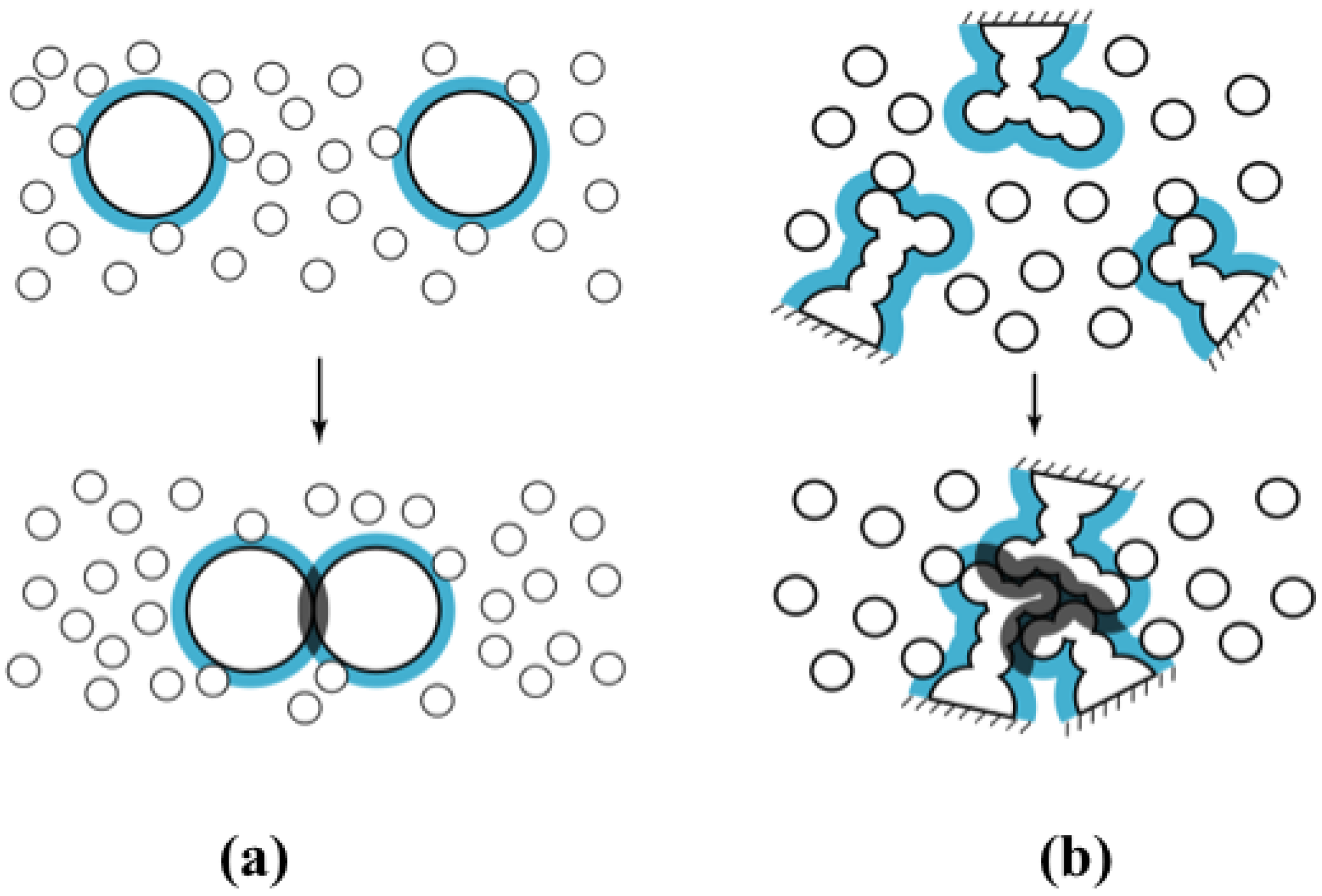
2.1. Major Driving Force of Protein Folding: Increase in Translational Entropy of Water

Most discussions concerning protein folding focus on contributions to the free-energy change that arise from potential energies among the atoms in the system, including the solvent [21]. An element lacking in earlier studies is that the translational movement (thermal motion) of the solvent molecules should critically influence the folding process. We begin with the concept illustrated in Figure 1a, which was first presented by Asakura and Oosawa [22]. Suppose that large particles are immersed in a bath of small particles and that the small and large particles are hard spheres with diameter d_S and diameter d_L, respectively. In such a system, all allowed configurations have the same energy and the system behavior is purely entropic in origin. The presence of a large particle generates the volume from which the centers of the small particles are excluded. The excluded volume is the spherical volume with diameter (d_L + d_S) that is the sum of the volumes of the large particle and of the envelope colored in blue (Figure 1a). When two large particles contact each other, the excluded volumes overlap (the overlapped volume is shadowed), and the total volume available to the translational movement of the small particles increases by the same amount. This increase leads to a gain in the translational entropy (TE) of the small particles. Within the framework of the Asakura–Oosawa (AO) theory, the free-energy change is given as −(ΔV/V_S)η_Sk_BT = −3(d_L/d_S)η_Sk_BT/2 [22,23], where η_S is the packing fraction of the small particles, ΔV the increase in the total volume available to the small particles defined above, V_S is the volume (size) of a small particle, and k_BT is Boltzmann’s constant times the absolute temperature. The gain in the TE of the solvent arising from contact is dependent not on the absolute value of the overlapped volume, but on the overlapped volume scaled by the size of the solvent molecules. In the isochoric process, the TE gain exactly equals the free-energy change divided by −T. In the isobaric process, there is a slight decrease in the system volume accompanying a corresponding decrease in the enthalpy. That is, part of the TE gain is converted into enthalpic gain. Irrespective of the process, the free-energy decrease originates purely from the TE effect in the model system considered [21,22]. In the original discussion by Asakura and Oosawa, the large particles are colloidal and the small particles are macromolecules. When the AO theory is applied to colloidal mixtures [23,24], the larger and smaller colloidal particles correspond to the large and small particles, respectively.

An important element of the concept described above is that the large particles are driven to contact each other by an increase in the TE and a decrease in the free energy of the system. Besides the highly specific steric and chemical interactions, this entropic effect is omnipresent in processes occurring in a condensed phase. In this study, we apply the concept to protein folding in water molecules that move energetically. In our application, the small and large particles are water molecules and a protein, respectively. In Figure 1b, three side chains are illustrated as an example of intramolecular contacts in the protein interior. The excluded volume for the solvent molecules and the overlapped volume are represented in the same manner as in Figure 1a. The geometric features of the side chains lead to a much larger overlapped volume than in the case of simple spheres (compare Figure 1a,b). The solvent in the biological system at the molecular level is water, whose molecular size is exceptionally small. For these reasons, the TE gain occurring in this particular system is expected to be quite substantial.

Figure 1. (a) Illustration of the concept first presented by Asakura and Oosawa [22]. (b) Application of the concept to protein folding occurring in solvent. In this example, three side chains are illustrated.

Figure 1. (a) Illustration of the concept first presented by Asakura and Oosawa [22]. (b) Application of the concept to protein folding occurring in solvent. In this example, three side chains are illustrated.

To investigate such TE effects in the protein/water system, we must employ a precise model and theory, rather than simply evaluating the change in excluded volume. For the first step, we can model solvent molecules and the protein molecule as hard sphere particles and a set of fused hard spheres, respectively, to account for the geometric features of the backbone and side chains at the atomic level. We employ three-dimensional (3D) integral equation theory [25,26], an elaborate statistical-mechanical approach that allows us to calculate the density structure of the solvent near a protein molecule in a prescribed conformation. These treatments enable us to exclusively investigate the TE by calculating the solvation free energy (SFE) because such a hard sphere system will not have an energy component arising from attractive inter-atomic interactions. Unlike AO theory, in which the free energy change is proportional to the excluded volume change, the TE obtained by our method reflects both the microscopic structure of the solvent density profile and the complex geometry of a solute molecule. It should be noted that the value of SFE, by definition, is irrespective of the thermodynamic process at work, i.e., isochoric or isobaric.

The key quantity we analyze is the TE of the solvent water in which the peptide or protein molecule is immersed. As an example, two peptides—Met-enkephalin (PDB ID: 1PLX) and the C-peptide fragment consisting of the 1–13 residues of ribonuclease A (PDB ID: 2AAS)—and two proteins—protein G (PDB ID: 2GB1) and barnase (PDB ID: 1BNR)—are considered. The TE gain upon folding is compared to CE loss. The CE change upon unfolding can roughly be estimated as the sum of (ln9)N_Rk_B and 1.7 N_Rk_B, which represent the contribution from the main chain and side chains of a protein, respectively [27]. We showed that when the number of residues is sufficiently large and the solvent is water (Figure 2), the TE gain is a powerful driving force and substantially competes against the very large CE loss [25,26].

We tested the native structure for protein G as well as numerous other conformations. The unfolded structures were generated using a molecular dynamic simulation with the all-atomic potentials [28]. The largest TE was attained in the native structure (Figure 3); the translational movement of water molecules is quite effective in achieving tight packing in the interior of a natural protein. These results are true only when the solvent is water, whose molecular size is among the smallest liquids in nature [25,26].

Figure 2. Gain in translational entropy (TE) of water calculated under the reference condition, and loss of conformational entropy (CE) of the peptide or protein molecule. TE gain and CE loss upon folding are compared. Entropy values are scaled by k_B.

Figure 2. Gain in translational entropy (TE) of water calculated under the reference condition, and loss of conformational entropy (CE) of the peptide or protein molecule. TE gain and CE loss upon folding are compared. Entropy values are scaled by k_B.

Figure 3. Solvation free energies obtained from 3D integral-equation theory for different structures of protein G (2GB1) as a function of the radius of gyration [28]. A total of 600 structures obtained from a molecular dynamic simulation are plotted.

Figure 3. Solvation free energies obtained from 3D integral-equation theory for different structures of protein G (2GB1) as a function of the radius of gyration [28]. A total of 600 structures obtained from a molecular dynamic simulation are plotted.

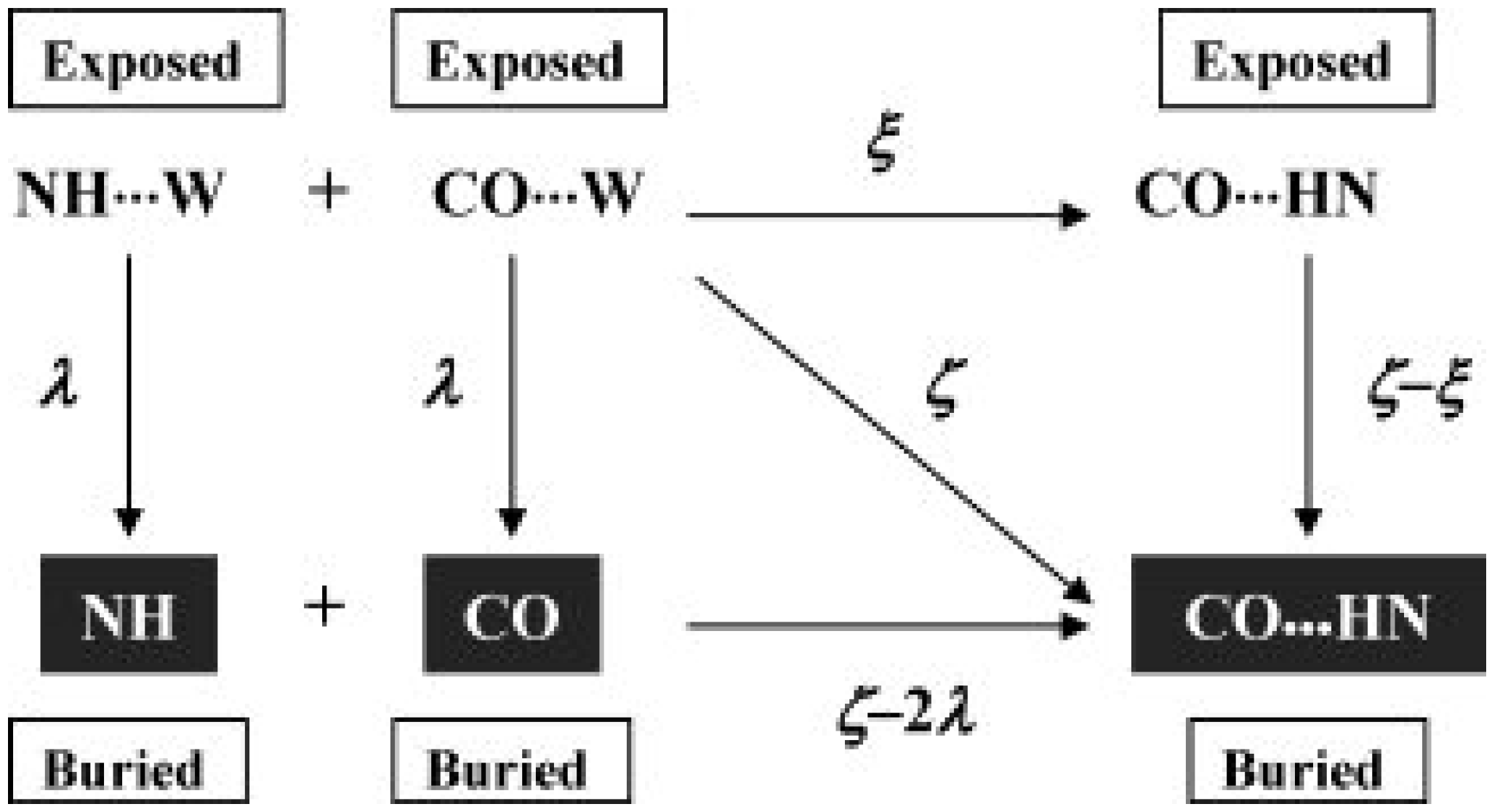
2.2. Free Energy Function Extracting the Physical Essence of Protein Stability

A physical factor that drives proteins to fold as described in the previous section with relation to the AO theory becomes apparent only when a protein is immersed in a condensed phase such as liquid water. This factor should be incorporated to evaluate the free energy change of the biological processes at the molecular level. One way to evaluate the effect is to estimate the hydration entropy for a realistic system consisting of the protein and water, starting from the energetics of the system, where a protein with a single fixed structure is immersed in water at infinite dilution [29]. Unrealistic structures in terms of internal energy, such as those with numerous overlaps of constituent atoms, are excluded from our discussion. The free energy of the system W can be expressed as the sum of the protein intramolecular energy E_intra and the hydration free energy μ: W = E_intra + μ, where μ consists of the hydration energy E_hyd and the hydration entropy S: μ = E_hyd − TS. Then, W = E_intra + E_hyd − TS, where T is the absolute temperature and μ is the same irrespective of the protein insertion condition in its definition (isobaric or isochoric) [30,31]. Hereafter, we consider the isochoric condition, which is much more convenient in a theoretical treatment.

The μ of several proteins, modeled with the all-atomic potential, were calculated by employing the three-dimensional reference interaction site model theory [32]. Their μ were decomposed into energetic and entropic components. The former comprises the protein-water interaction energy and the water reorganization energy arising from the structural changes of a solute. Each component was further decomposed into nonelectrostatic and electrostatic contributions, and it was shown that μ was governed by the nonelectrostatic component of S and the electrostatic component of E_hyd. The change in S was less than 5% even when protein-water electrostatic interactions, which are long-range and quite strong, are completely shut off. S asymptotically becomes proportional to the excluded volume for water molecules as the protein size increases. This result is consistent with the study using angle‑dependent integral equation theory for hydration thermodynamics of a simple solute model, indicating that S for a larger solute is determined primarily by the translational component [33]. On the basis of the great advantage that S is not significantly influenced by interactions between protein and water, we can model a protein molecule as a set of fused hard spheres mimicking constituent atoms. However, it should be emphasized that an explicit molecular model for water (i.e., not a dielectric continuum model) must be employed in the calculation of S.

Contrary to S, “E_intra + E_hyd” is quite sensitive to changes in interactions between protein and water. According to studies using an all-atomic molecular model [34], there is a tendency for ΔE_intra and ΔE_hyd to compensate for each other upon structural changes in a protein (i.e., their magnitudes are close to each other and their signs are opposite). Therefore, instead of accounting for all atomic interactions, “E_intra + E_hyd” is evaluated by comparing the energy difference due to structural changes in the solute molecule, which are accompanied by the change in hydration energy. Thus, we assume that hydrogen bonds will have a major contribution. A fully extended protein structure is chosen as the reference. Such a structure should possess the maximum number of hydrogen bonds with water molecules and no intramolecular hydrogen bonds in the protein. When a protein folds into a compact structure, some proton donors or acceptors (e.g., N and O, respectively) are buried in the interior after hydrogen bonds with water molecules (CO···W, NH···W, etc.) are broken. If the donors or acceptors cannot form hydrogen bonds in the protein interior, we can impose a dehydration penalty. Our basic concept is illustrated with the thermodynamic cycle in Figure 4. Let Λ denote the total dehydration penalty (TDP). When compared with the fully extended structure (Λ = 0), a more compact structure has some donors and acceptors buried in its interior, leading to some positive value of Λ depending on the protein conformation. We can equate “E_intra + E_hyd” with the TDP occurring upon transition to a more compact structure if intramolecular hydrogen bonds are not completely formed. The free energy function F is given by:

F = −TS + Λ

(1)

Based on the thermodynamic treatments described above, we can construct an energy function for an all-atomic molecular model that captures the essential thermodynamics of protein folding despite its simplicity. It suggests that the native structure should be the fold with the lowest value of the energy function if it is constructed in a physically reasonable manner. One advantage is that our function is free from differences in van der Waals attraction or Coulombic force parameters. Moreover, it is calculated with minor computational effort, as described in the next subsection.

Figure 4. The scheme for calculating the total dehydration penalty. “W” and “···” represent a water molecule and a hydrogen bond, respectively. An amide NH and CO are depicted as an example. The parameters ζ, λ, and ξ are changeable.

Figure 4. The scheme for calculating the total dehydration penalty. “W” and “···” represent a water molecule and a hydrogen bond, respectively. An amide NH and CO are depicted as an example. The parameters ζ, λ, and ξ are changeable.

2.3. Computational Methods & Molecular Models

Because F must be evaluated for a great number of conformations, the calculation of F per structure should be performed with low computational cost and the essential role of water should be accounted for as well. We have developed a judicious method meeting both requirements.

The hydration entropy, which strongly depends on the details of the protein polyatomic structure, is calculated using a hybrid of the angle-dependent integral equation theory [35,36,37,38,39], i.e., a statistical-mechanical theory for molecular liquids, and the morphometric approach [28]. In the angle-dependent integral equation theory, the role of water as a molecular ensemble is fully considered. The water-water and solute-water orientational correlations are fully taken into account. Next, the multi-polar model [40] is employed to mimic water molecules. The solute-solvent (water) pair correlation function can be denoted by g(r, θ, φ, χ), where r is the distance from the center of the solute, (θ, φ) represents the orientation of the dipole moment of the vector water (θ is the angle between the vector and the solute‑water axis), and χ describes the rotation around the dipole-moment vector. The Morita–Hiroike formula [41,42] for calculating the hydration free energy μ is written as:

$$\begin{array}{c}\mu =\frac{k_{\text{B}}T\rho }{8{\pi }^2}{\displaystyle \int {\displaystyle \int {\displaystyle \int {\displaystyle \int 4\pi [\frac{1}{2}{\left\{h\left(r,\theta ,\varphi ,\chi \right)\right\}}^2}}}}\\ -\frac{1}{2}h\left(r,\theta ,\varphi ,\chi \right)c\left(r,\theta ,\varphi ,\chi \right)-c\left(r,\theta ,\varphi ,\chi \right)]r^2\sin \theta drd\theta d\varphi d\chi \end{array}$$

(2)

where h(= g – 1) and c are the total and direct correlation functions, respectively. The integral range is [0, ∞] for r, [0, π] for θ, and [0, 2π] for ϕ and χ; k_B and ρ are the Boltzmann constant and the number density of solvent water, respectively. As mentioned in the methods section, S is considered under an isochoric condition and calculated through the thermodynamic relation:

$$S=-\left(\frac{\partial \mu }{\partial T}\right)$$

(3)

Temperature derivatives are numerically evaluated from:

$$\left(\frac{\partial \mu }{\partial T}\right)=\frac{\mu \left(T+\delta T\right)-\mu \left(T-\delta T\right)}{2\delta T}$$

(4)

where δT = 5 K is adopted.

Although employing this theory is computationally expensive, the calculation of hydration entropy for a protein is quite rapid while still being in quantitative agreement with morphological thermodynamics [28]. This combined method requires minor computational time while retaining quantitative accuracy. The idea of our morphometric approach is to express a hydration quantity such as S using a linear combination of only four geometric measures of a solute molecule:

$$S=c_{\text{1}}V+c_{\text{2}}A+c_{\text{3}}C+c_{\text{4}}X$$

(5)

where V, A, C and X correspond to the excluded volume, solvent accessible surface area, integrated mean and Gaussian curvature, respectively [28]. In our approach, the solute shape enters S only via the four geometric measures. Therefore, the four coefficients (c₁ − c₄) can be determined using a simple geometry: They are determined in advance from the values of S for hard-sphere solutes with various diameters (d_solute: 0≤ d_solute ≤10 d_water, where d_water denotes the diameter of a water molecule) immersed in our model water. Angle-dependent integral equation theory is employed in the calculation. The four coefficients are determined by a least-squares fit applied to the following equation for hard-sphere solutes:

$$S=c_1\left(4\pi R^3/3\right)+c_2\left(4\pi R^2\right)+c_3\left(4\pi R\right)+c_4\left(4\pi \right)$$

(6)

where R = (d_solute + d_water)/2. The values of the four coefficients thus obtained are the following: C₁= −0.1971 Å⁻³, C₂ = 0.06119 Å⁻², 4πC₃ = 1.967 Å⁻¹, and 4πC₄ = −2.652. It should be noted that S determined by this procedure contains a rotational component even though, as stated above, it becomes minor for a large molecule. As explained in the text, we can model a protein structure as a set of fused hard spheres. Each diameter is the Lennard–Jones (LJ) σ-parameter corresponding atom, which is taken from the typical force field. Once determined for simple hard spheres, the four coefficients can be used to calculate S for a protein with any structure by calculating the four geometric measures for each protein structure using the Connolly algorithm [38]. The x-y-z coordinates of the protein atoms, which characterize each structure on the atomic level, are used as part of the input data for calculating the four geometric measures.

Our basic strategy for calculating the TDP is illustrated in Figure 4. When a donor and acceptor are buried in the interior after breakage of exterior hydrogen bonds with water molecules, we impose a penalty or gain of ζ if they form an intramolecular hydrogen bond. On the other hand, when a donor or an acceptor is buried with no intramolecular hydrogen bond formed, we only impose a penalty of λ. The formation of an intramolecular hydrogen bond exposed to water is assumed to accompany a penalty or gain of ξ. The formation of an intramolecular hydrogen bond within the interior leads to the gain of ζ − 2λ. The burial of an intramolecular hydrogen bond is accompanied by a penalty or gain of ζ − ξ. It should be noted that λ is positive and quite large. We examine whether each donor and acceptor in the backbone, backbone-and side chain can form intramolecular hydrogen bonds, and it is necessary to determine whether each donor or acceptor is buried. The water-accessible surface area is calculated for each of them using Connolly’s algorithm [43]. If it is smaller than the threshold value, the donor or acceptor is considered buried. The threshold is set at 0.001 Ų. To determine whether the hydrogen bond is formed, i.e., if the bond length and angle are within appropriate ranges, the criteria proposed by McDonald and Thornton [44] are used.

In studying protein stability, we assume that (λ, ξ, ζ) can be set at (7k_BT₀, 0, 0) (T₀ = 298 K) based on results from Brooks and coworkers [45], who performed a molecular dynamics simulation for hydrogen-bond formation between two formamide molecules in a nonpolar liquid and in water. In this setting, we impose no penalty when a donor and an acceptor are buried in the interior, if they form an intramolecular hydrogen bond. When a donor or an acceptor is buried with no intramolecular hydrogen bond formed, we impose a penalty of 7k_BT₀. The setting λ = 7k_BT₀ is also consistent with the estimation by Fleming and Rose [46] of 5–6 kcal/mol (∼10k_BT₀). However, it should be noted that the slight difference in these values concerning the TDP does not affect the overall profile of the energetics. The computation of Λ per protein structure is simply a count of the number of such donors or acceptors and is rapidly computed. It becomes apparent that no dehydration penalty is paid by the nonpolar groups of a protein. This can be justified because the breakage of hydrogen bonds with water molecules is more important and forms a principal component of the TDP when not compensated for by intramolecular hydrogen bonds.

3. Validation of the Free Energy Function

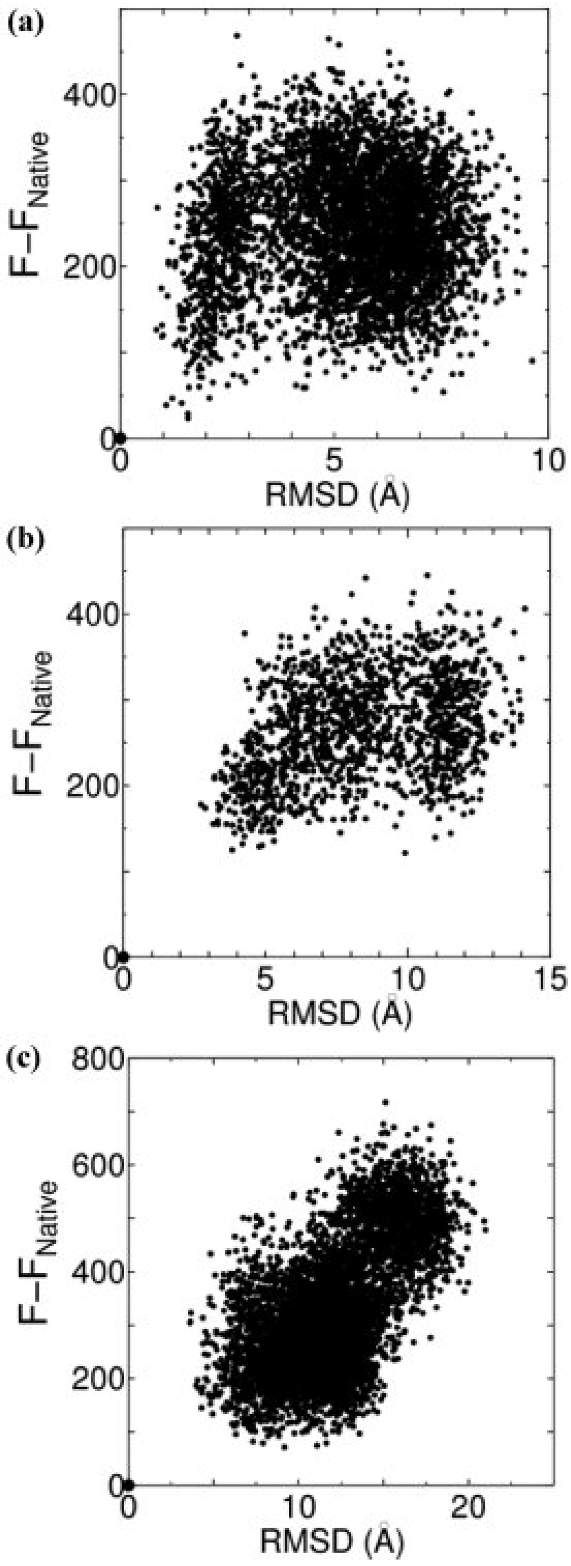
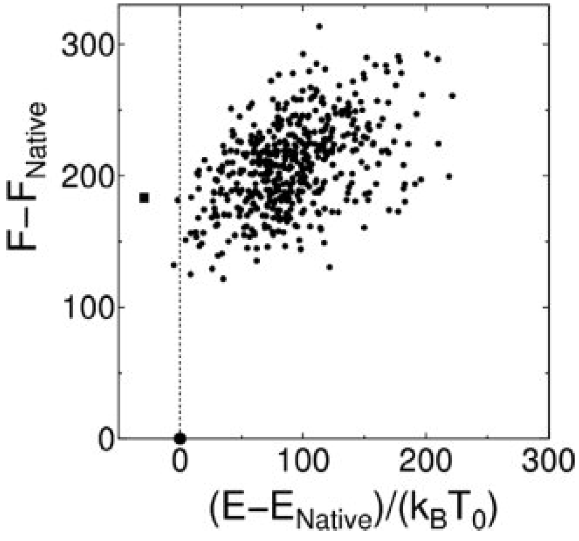
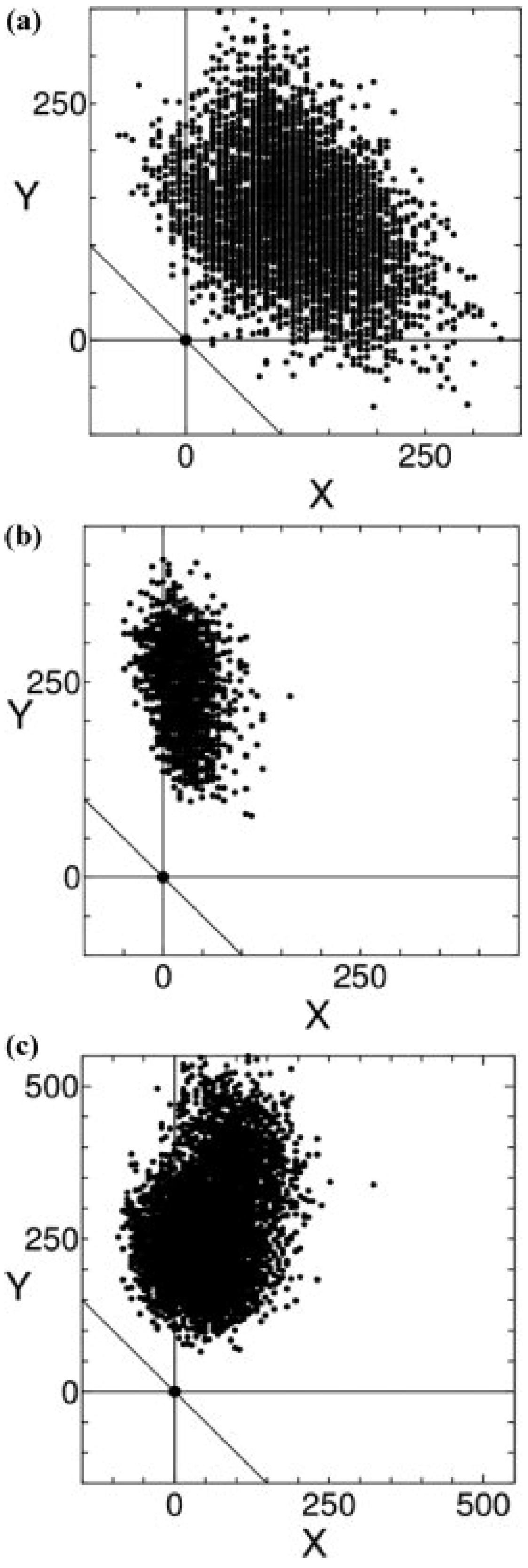
3.1. Discrimination of the Native Structures from Misfolded Decoys

As a first step, we must validate the free energy function by comparing the experimentally determined “native” structure to a vast number of possible conformations. “Decoys” are protein conformations that are computationally generated and possess some characteristics of native proteins, but are not biologically real. The primary use of decoy structures is to test scoring or newly developed energy functions. If the function can discriminate the native structure as that with the lowest value, our treatment of energetics for protein hydration thermodynamics is validated [29,47,48]. We tested the discrimination ability with the decoy sets 4state_reduced [49], fisa, fisa_casp3 [50], Rosetta [51], lattice_ssfit [52,53], lmds [54], and Semfold [55], which are maintained in a database at [56]. We omit the set of 1fc2 in fisa because the structure referred to as “the native fold” is only a fragment of the protein A complex in the experiment. The free-energy function should be evaluated not for the fragment but for the complex. However, the decoy set for this entry was generated only for the fragment. This aspect is discussed in the next subsection.

Each decoy structure is slightly modified to eliminate unrealistic overlaps between constituent atoms. Metal ions such as calcium (Ca²⁺) or zinc (Zn²⁺) are entangled in the experimental structure. Although some proteins structures are heme-binding (i.e., have covalent linkages with heme), neither the ion nor heme is included in the decoy structures. The detailed procedures are described in the appendix of [48].

In this study, we exclude structures determined by nuclear magnetic resonance (NMR) due to their conformational ambiguity. NMR structures are usually deposited in the PDB as a collection of models that satisfy geometrical restrains. Typically, the models are composed of a structurally conserved core region and a variable region (loops and chain terminals). The variable region may have structural difference as large as 5 Å in Cα RMSD. Additionally, the final structures are computationally determined through energy optimization of the force fields, which define the distance constraints between constituent atoms [57]. Therefore, the results may largely depend on both the optimization procedure and the force fields. Because our goal is to compare the score of a native structure with a decoy structure, it is crucial to have one well-defined native structure with the least bias in favor of other force fields. The calculated F values for the candidates vary widely from model to model even though they are deposited as a native structure, so we also omitted some decoy sets from our discussion if the native structures were determined with NMR.

The plot of F − F_Native (the subscript “Native” denotes the value for the native structure) against the root mean square displacement (RMSD) for Cα atoms from the native structure is shown for the three representative decoy sets in Figure 5. The data for all of the protein species contained in each decoy set are collected in the figure. In Table 1, the number of decoy sets for which our energy function identifies the native structure as the lowest value is listed. As observed in the table, our function is successful in discriminating the native fold from misfolded decoys with 100% accuracy, except for lmds decoy sets (the lack of success in these decoy sets is justified in the next subsection). This success supports our arguments around hydration, described above, and the validity of the energy function.

To compare the discrimination performance, the measure called the Z-score [58,59] is used, which is defined by:

$$Z=(F_{Native}-<F>)/F_{\sigma }$$

(7)

where < F > is the energy function averaged over all structures and F_σ the standard deviation. As easily recognized from the form of Equation (7), the larger the magnitude of the Z-score is, the more successful the result.

Figure 5. F − F_Native plotted against Cα-RMSD from the native structure. Each figure collects data for all proteins in the decoy set of 4state_reduced (a), fisa (b), and fisa_casp3 (c). Native structures are represented by the origin (0, 0) of the plots.

Figure 5. F − F_Native plotted against Cα-RMSD from the native structure. Each figure collects data for all proteins in the decoy set of 4state_reduced (a), fisa (b), and fisa_casp3 (c). Native structures are represented by the origin (0, 0) of the plots.

The performance of our free-energy function is compared with that of the scoring functions previously proposed by other research groups in Table 1, in terms of the number of successful sets and the averaged Z-score for each decoy set. The Z score shows that our function gives the highest performance among scoring functions compared here. We note that the function of Lu et al. [60], a knowledge-based function, has been shown to give the best result among the functions available in the literature. In the scoring function of Lu et al., emphasis is placed on the side-chain packing. It is known that side chains are tightly packed in the native structure, with little space in its interior. As illustrated in Figure 1, such a feature leads to nearly the highest entropy of water. Tight packing is thought to be driven by van der Waals interactions among the protein atoms. We note, however, that burial or packing results in a loss of van der Waals interaction energy between the protein and solvent water and that burial and packing can be driven by water-entropy gain. In this sense, the scoring function of Lu et al. is closely related to our free-energy function, though it has its origin in a structural database. Judging by the almost equal success of the potential function of Lu et al. when compared with our free-energy function, the water-entropy effect is a crucially important factor in the energetics of protein stability.

Table 1. The performance of F in comparison with the scoring functions previously proposed. The number of successful decoy sets and the averaged Z-score for each decoy set.

Scoring Function	Top1/Total No.	Mean Z
4state_reduced
F	7/7	−5.19
Lu et al., 2008 [60]	7/7	−4.41
Miyazawa and Jernigan, 2005 [61]	7/7	−4.44
Lee and Duan, 2004 [62]	7/7	−4.95
Zhang et al., 2004 [63]	6/7	−3.94
Onizuka et al., 2002 [64]	7/7	−3.41
Zhou and Zhou, 2002 [65]	6/7	−3.49
Toby and Elber, 2000 [66]	3/6	−3.14
Fisa
F	3/3	−6.97
Lu et al., 2008 [60]	3/3	−5.52
Miyazawa and Jernigan, 2005 [61]	2/4	−2.55
Lee and Duan, 2004 [62]	2/3	−3.73
Zhang et al., 2004 [63]	3/4	−4.70
Onizuka et al., 2002 [64]	1/3	−1.38
Zhou and Zhou, 2002 [65]	3/3	−5.91
Toby and Elber, 2000 [66]	2/3	−3.34
Fisa_casp3
F	5/5	−5.51
Lu et al., 2008 [60]	5/5	−5.35
Miyazawa and Jernigan, 2005 [61]	2/5	−3.61
Lee and Duan, 2004 [62]	2/5	−3.19
Zhang et al., 2004 [63]	3/3	−6.05
Onizuka et al., 2002 [64]	1/3	−2.01
Zhou and Zhou, 2002 [65]	3/3	−5.37
Toby and Elber, 2000 [66]	1/3	−2.01
Rosetta (X-ray)
F	41/41	−7.12
Lu et al., 2008 [60]	37/41	−6.56
lattice_ssfit
F	8/8	−7.54
Miyazawa and Jernigan, 2005 [61]	8/8	−11.12
Lu et al., 2008 [60]	8/8	−6.52
Lmds
F	9/10(10/10)	−6.29 (−6.79)
Miyazawa and Jernigan, 2005 [61]	8/10	−5.34
Lu et al., 2008 [60]	8/10	−5.20
Semfold
F	8/8	−6.76
Miyazawa and Jernigan, 2005 [61]	4/6	−3.86

Table 1. The performance of F in comparison with the scoring functions previously proposed. The number of successful decoy sets and the averaged Z-score for each decoy set.

Scoring Function	Top1/Total No.	Mean Z
4state_reduced
F	7/7	−5.19
Lu et al., 2008 [60]	7/7	−4.41
Miyazawa and Jernigan, 2005 [61]	7/7	−4.44
Lee and Duan, 2004 [62]	7/7	−4.95
Zhang et al., 2004 [63]	6/7	−3.94
Onizuka et al., 2002 [64]	7/7	−3.41
Zhou and Zhou, 2002 [65]	6/7	−3.49
Toby and Elber, 2000 [66]	3/6	−3.14
Fisa
F	3/3	−6.97
Lu et al., 2008 [60]	3/3	−5.52
Miyazawa and Jernigan, 2005 [61]	2/4	−2.55
Lee and Duan, 2004 [62]	2/3	−3.73
Zhang et al., 2004 [63]	3/4	−4.70
Onizuka et al., 2002 [64]	1/3	−1.38
Zhou and Zhou, 2002 [65]	3/3	−5.91
Toby and Elber, 2000 [66]	2/3	−3.34
Fisa_casp3
F	5/5	−5.51
Lu et al., 2008 [60]	5/5	−5.35
Miyazawa and Jernigan, 2005 [61]	2/5	−3.61
Lee and Duan, 2004 [62]	2/5	−3.19
Zhang et al., 2004 [63]	3/3	−6.05
Onizuka et al., 2002 [64]	1/3	−2.01
Zhou and Zhou, 2002 [65]	3/3	−5.37
Toby and Elber, 2000 [66]	1/3	−2.01
Rosetta (X-ray)
F	41/41	−7.12
Lu et al., 2008 [60]	37/41	−6.56
lattice_ssfit
F	8/8	−7.54
Miyazawa and Jernigan, 2005 [61]	8/8	−11.12
Lu et al., 2008 [60]	8/8	−6.52
Lmds
F	9/10(10/10)	−6.29 (−6.79)
Miyazawa and Jernigan, 2005 [61]	8/10	−5.34
Lu et al., 2008 [60]	8/10	−5.20
Semfold
F	8/8	−6.76
Miyazawa and Jernigan, 2005 [61]	4/6	−3.86

It is worthwhile to compare our free energy function with a representative physics-based function. Here, we employ CHARMM, one of the most widely used force fields, which includes the CHARMM22 [67] + CMAP [68] (MM) + Generalized-Born Approximation [69,70,71] (GBMV) +Accessible Surface Area method (SA). The GBMV is reportedly capable of reproducing the potential energy calculated by the Poisson–Boltzmann method and that from the molecular dynamics simulation combined with an explicit water model. The MM+GBMV/SA tested does not always successfully discriminate the native structure from the decoys. We found a typical case in the decoy set for 1hdd-C. The relation between our function F and MM+GBMV/SA is shown for 1hdd-C in the fisa decoy set in Figure 6. The F generally gives much higher energy values for all the decoy structures than does MM+GBMV/SA. As observed in the figure, there are two decoy structures for which MM+GBMV/SA identifies lower energy values than the native. These two structures contain more α-helical structure than the native structure. In Figure 6, one of the two decoy structures is illustrated for comparison with the native structure. We explore the relation between the α-helix content and the energy value of our function and MM+GBMV/SA. A hypothetical all α-helix structure was also considered (Figure 7). As observed in Table 2, MM+GBMV/SA values tend to be lower for structures with higher α-helix content. The present result is consistent with studies showing that the CHARMM22 force-field parameters have a preference for α-helix conformations [72,73]. The hydration entropy in our free‑energy function of the decoy structures is much larger than that of the native structure. It is quite reasonable that all α-helix structures, which have a relatively larger excluded volume for water, is unfavorable in terms of the hydration entropy [25,26]. The water entropy for the decoy structure is lower than that for the native structure by ∼98 k_B. In contrast, an all α-helix structure has less dehydration penalty than a native structure because it can form intramolecular hydrogen bonds in a complete manner. The relation between structure and energy terms is discussed in the next subsection.

Figure 6. Relation between F − F_Native and (E − E_Native)/(k_BT₀) for 1hdd-C in the fisa decoy set. F (note that this is already scaled by k_BT₀; T₀ = 298 K) is our free-energy function, and E is the CHARMM22+CMAP+GBMV/SA. The square and the large circle represent the result of an all α-helix structure and the native structure, respectively.

Figure 6. Relation between F − F_Native and (E − E_Native)/(k_BT₀) for 1hdd-C in the fisa decoy set. F (note that this is already scaled by k_BT₀; T₀ = 298 K) is our free-energy function, and E is the CHARMM22+CMAP+GBMV/SA. The square and the large circle represent the result of an all α-helix structure and the native structure, respectively.

Figure 7. Ribbon representation of examined protein structures. (a) The native structure of 1hdd-C. (b) Structure with the lowest value of CHARMM22+CMAP+GBMV/SA in the decoy set. (c) All α-helical structure with the same amino-acid sequence.

Figure 7. Ribbon representation of examined protein structures. (a) The native structure of 1hdd-C. (b) Structure with the lowest value of CHARMM22+CMAP+GBMV/SA in the decoy set. (c) All α-helical structure with the same amino-acid sequence.

Table 2. Comparison among the native, decoy, and all α-helix structure in terms of α‑helical content, the energy value of CHARMM22 (MM+GBMV/SA), hydration entropy (S), total dehydration penalty (Λ), and our free energy function (F). All values are relative to the corresponding native energy values.

Structure	α-helical Content (%)	MM+GBMV/SA/(kBT0)	−S	Λ	F
Native	74	0.0	0.0	0.0	0.0
Decoy	79	−5.7	97.5	35	132.5
All α	100	−29.1	204.5	−21	183.5

Table 2. Comparison among the native, decoy, and all α-helix structure in terms of α‑helical content, the energy value of CHARMM22 (MM+GBMV/SA), hydration entropy (S), total dehydration penalty (Λ), and our free energy function (F). All values are relative to the corresponding native energy values.

Structure	α-helical Content (%)	MM+GBMV/SA/(kBT0)	−S	Λ	F
Native	74	0.0	0.0	0.0	0.0
Decoy	79	−5.7	97.5	35	132.5
All α	100	−29.1	204.5	−21	183.5

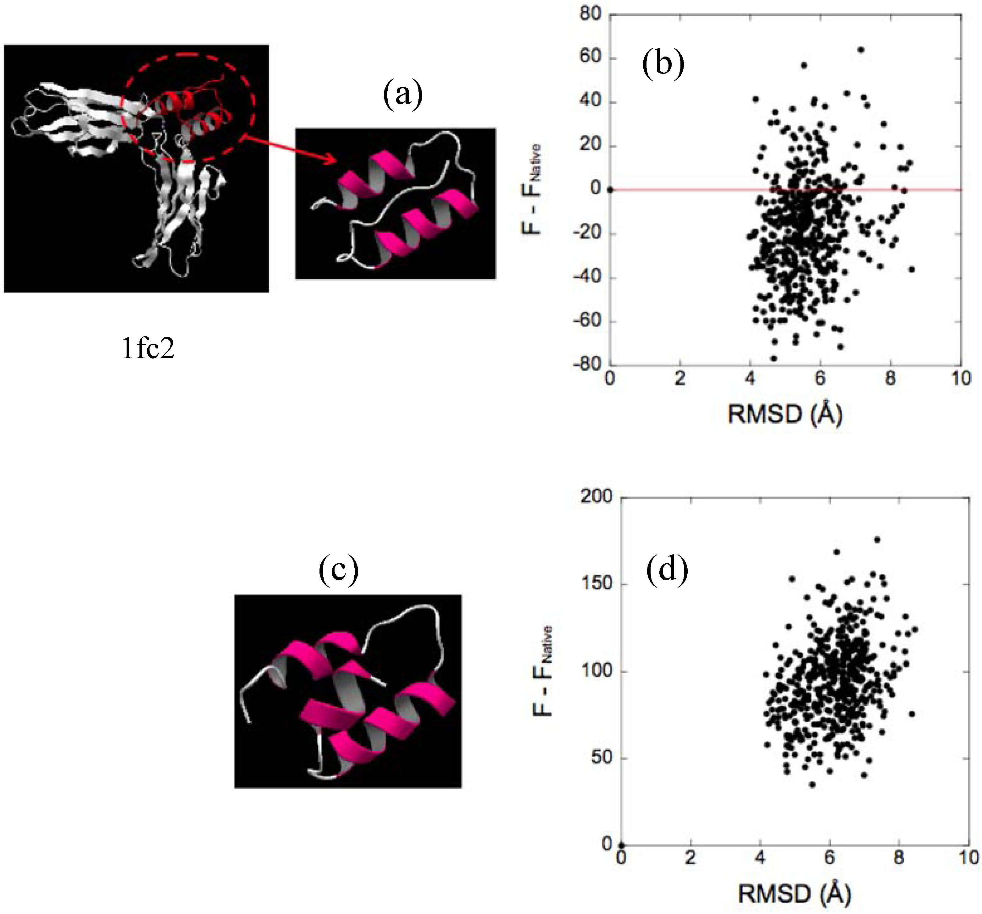
3.2. Characteristics of Native Proteins

We define X and Y by:

$$X=\Lambda /(k_{\text{B}}{T}_0)-{\left\{\Lambda /(k_{\text{B}}{T}_0)\right\}}_{Native}$$

(8)

and:

$$Y=-TS/(k_{\text{B}}{T}_0)-{\left\{-TS/(k_{\text{B}}{T}_0)\right\}}_{Native}$$

(9)

respectively, where the subscript ‘Native’ denotes the value for the native structure. The plot of Y against X is shown in Figure 8, and considered data for all of the decoy sets. There are many structures with X < 0. Some structures give Y < 0 only in the 4state_reduced decoy set. This result suggests that the full consideration of the water-entropy effect is crucially important in characterizing the native structure. In any case, there is no structure with X + Y < 0. Structures that have higher entropy of water than the native structure can certainly be constructed, but such structures suffer serious total dehydration penalties. Structures with less total dehydration penalty than the native structure can also be constructed (e.g., all α-helix structure), but such structures give rise to a rather low entropy of water. The native structure is optimized in terms of the sum of the two important factors. We emphasize, however, that the major driving force in protein folding is the gain in water entropy, especially when the folding process is considered under the isochoric condition. (Under the isobaric condition, part of the entropic gain is converted to a corresponding enthalpy gain. Refer to our publication [31] for more details.) The formation of intramolecular hydrogen bonds is important for reducing the dehydration penalty as much as possible during the folding process and leads to the formation of common motives found in the secondary structure of proteins, i.e., α-helix or β-sheet.

Figure 8. Y plotted against X for all the proteins in the 4state_reduced (a), fisa (b), and fisa_casp3 (c) decoy sets, defined by Y = −TS/(k_BT₀) − {−TS/(k_BT₀)}_Native and X = Λ/(k_BT₀) − {Λ/(k_BT₀)}_Native, respectively. The three straight lines represent X = 0, Y = 0, and X + Y = 0, respectively.

Figure 8. Y plotted against X for all the proteins in the 4state_reduced (a), fisa (b), and fisa_casp3 (c) decoy sets, defined by Y = −TS/(k_BT₀) − {−TS/(k_BT₀)}_Native and X = Λ/(k_BT₀) − {Λ/(k_BT₀)}_Native, respectively. The three straight lines represent X = 0, Y = 0, and X + Y = 0, respectively.

We found the evidence for how well F discriminated between the stable structures of a protein. In the lmds decoy set, one decoy structure is constructed for a native structure where the two fragments take a complex form as illustrated in Figure 9a. Their atomic coordinates are defined not for the complex but for the fragment (i.e., chain C of the PDB structure with code 1fc2). Such decoy structures are entered as the decoy set for 1fc2. If the structure of the fragment is assumed to remain unchanged even when isolated and regarded as the model of the native protein, there are a number of decoy structures whose F value is lower than that of the native model (Figure 9b). The Z-score is calculated as 0.76, but this treatment for the native model leads to failure, as reflected in 9/10 and −6.29 for the lmds decoy set in Table 1. The structure of the fragment was determined using NMR in its isolated form in aqueous solution (The PDB code is 1bdc) and is considerably different from the native model as illustrated in Figure 9c (it contains one more α-helix). The structure of 1dbc must be defined as the reference native structure. With this definition, our function gives the lowest value for the native, as shown in Figure 9d, and the Z-score for this decoy set becomes −4.15. This alteration is identified as a success and reflected in (10/10) and (−6.79) for the lmds decoy set in Table 1. These results indicate that the features of the experimentally determined native structure (i.e., it is optimized in terms of the sum of the two important factors) are precisely captured by our function.

Figure 9. (a) Ribbon representation of chain C structure in the complex (PDB code: 1fc2). (b) F − F_Native plotted against Cα-RMSD from the native structure. Chain C of the PDB structure with code 1fc2 used as the native. (c) Ribbon representation of 1bdc. Chain C of 1fc2 is isolated in aqueous solution, and its structure is determined using NMR spectroscopy and deposited to PDB as 1bdc. (d) F − F_Native plotted against Cα-RMSD from 1bdc as the native structure.

Figure 9. (a) Ribbon representation of chain C structure in the complex (PDB code: 1fc2). (b) F − F_Native plotted against Cα-RMSD from the native structure. Chain C of the PDB structure with code 1fc2 used as the native. (c) Ribbon representation of 1bdc. Chain C of 1fc2 is isolated in aqueous solution, and its structure is determined using NMR spectroscopy and deposited to PDB as 1bdc. (d) F − F_Native plotted against Cα-RMSD from 1bdc as the native structure.

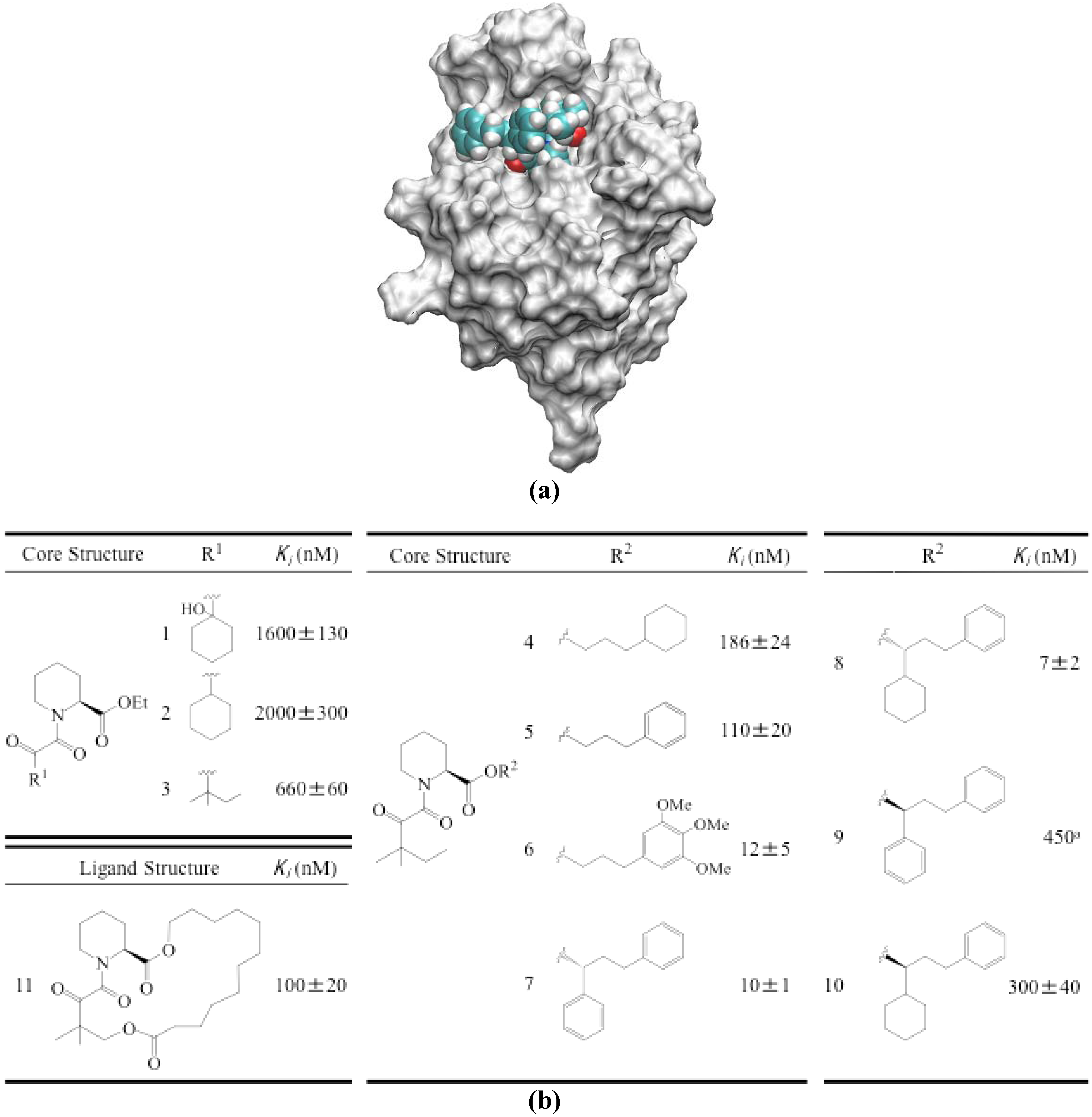
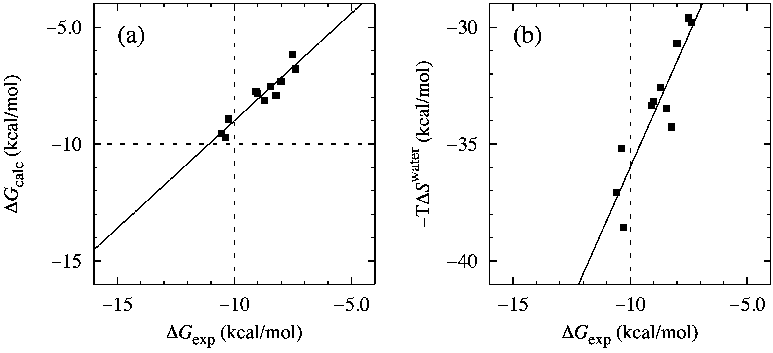
3.3. Evaluation of Protein-Ligand Binding Free Energy

The energetics of protein folding can be applied to binding between a ligand and a receptor protein because the change in hydration for such processes should be the same in terms of the molecular association in solvent water. The difference is only whether it denotes an intermolecular or an intramolecular change. However, this change in configuration entropy should additionally be considered in the energetics of the binding process as follows [74].

For a protein-ligand binding process in aqueous solution, the free-energy change is given by:

$$\Delta G=G_{complex}-G_{protein}-G_{ligand}$$

(10)

Here, we introduce the assumption in hydration thermodynamics described in the Introduction: In Equation (10), the energetic components are replaced by the dehydration penalty, Λ. Equation (10) is then written as follows:

$$\Delta G=\Delta \Lambda -T{S}_{complex}+(T{S}_{protein}+T{S}_{ligand})$$

(11)

In the case of intermolecular association, the conformational change of protein and ligand upon their binding are considered. Each entropic component can be decomposed into two terms: one from the solute alone and the other from water-entropy loss upon solute insertion. The former corresponds to the configuration entropy of the solute and is hereafter denoted by S^config. The latter corresponds to the solvation entropy of a solute and is denoted by S^water. Thus, the free-energy change ΔG for protein-ligand binding in aqueous solution is given by:

$$\begin{array}{c}\Delta G=\Delta \Lambda -(T{S}_{complex}^{config}+T{S}_{complex}^{water})+(T{S}_{protein}^{config}+T{S}_{protein}^{water})\\ +(T{S}_{ligand}^{config}+T{S}_{ligand}^{water})\\ =\Delta \Lambda -(T{S}_{complex}^{config}-T{S}_{protein}^{config}-T{S}_{ligand}^{config})\\ -(T{S}_{complex}^{water}-T{S}_{protein}^{water}-T{S}_{ligand}^{water})\\ =\Delta \Lambda -T\Delta S^{config}-T\Delta S^{water}\\ =\Delta F-T\Delta S^{config}\end{array}$$

(12)

ΔG is regarded as the binding free energy (BFE) between a protein and a ligand. S^water for each structure of a solute molecule is calculated with the computational process described above. The structures are taken from snapshots of a trajectory generated with molecular dynamics simulations. In this study, we employ the so-called single-trajectory approach [75] to obtain structural ensembles of the protein, ligand, and their complex; namely, we perform a single MD simulation for the complex to obtain snapshot structures. The snapshot structures of the protein and ligand are extracted from the same trajectory data. Thus, the final value of S^water is an average of S^water for each structure. If a protein does not accompany large conformational change upon binding, S^config can be regard as local fluctuation around a fixed structure. To estimate S^config, suppose that the solute has N conformations, each of which can be treated as a disjoint multidimensional harmonic well. We can calculate S^config using the following equation [76]:

$$S_X^{config}=-R{\displaystyle \sum _j{p}_j\ln p_j}+{\displaystyle \sum _j{p}_j{S}_{X,j}^{config}}$$

(13)

where p_j represents the probability that a conformation belongs to well j. S_X,j^config corresponds to the local entropy of well j including translational, rotational, and vibrational entropies. Here, we omitted the first term on the right-hand side of Equation (13) because a change in the first term upon ligand binding would be negligible compared with that of the second term [71]. In calculating the local entropy of well j, S_config in Equation (13), the Hessian matrix is necessary for each local minimum structure. We then perform the optimization of geometry for each sampled structure by the conjugate gradient method followed by the Newton–Raphson method. During the optimization, the solvation effect is taken into account with a continuum model known as the generalized Born method [77]. The structures thus obtained are subjected to normal mode analysis to calculate the vibration entropy. It should be emphasized that we performed normal mode analysis for the full atomic protein structure. We used standard statistical mechanics formulas for an ideal gas to calculate translational and rotational entropies. Note that these entropic contributions are minor for the relative value, as shown later.

In the study of the BFE, we incorporate ΔΛ in the following manner. Before forming a complex, the protein and ligand are both fully hydrated, which means that the proton donors and acceptors on their surfaces form hydrogen bonds with the surrounding water molecules. Upon ligand binding, some of these hydrogen bonds are replaced by newly formed protein-ligand hydrogen bonds. If all of the protein-water or ligand-water hydrogen bonds lost upon complex formation are compensated by the protein-ligand hydrogen bonds, there is no dehydration penalty. However, when a donor or an acceptor is buried with no protein-ligand hydrogen bond formed, a dehydration penalty should be imposed.

Here, we apply our energetics to protein-ligand binding systems. The system studied here comprises FK506-binding protein 12 (FKBP12) and its 11 ligands (Figure 10). The BFEs between FKBP12 and its inhibitors have been experimentally determined and studied by several research groups using different computational methodologies [78,79,80,81,82,83], making the system appropriate as the first choice for a benchmark study. We confirmed the MD simulation on this system shows no large conformational change upon binding [74]. Therefore, the treatment for S^config described above is suitable for the system. FKBP12 is a small protein of 107 residues with five anti-parallel β-strands wrapping around a short α-helix to form an overall barrel shape. The binding site consists of Tyr26, Phe36, Phe46, Val55, Ile56, Trp59, Tyr82, His87, Ile90, and Phe99, all of which are buried inside upon binding. A crystallographic structure study [84] revealed that two water molecules (WAT186 and WAT125 in the PDB file of 1FKG) bind to the hydroxyl group of Tyr82 in the FKBP12 and are displaced with ligand #7 upon the formation of a complex. In the structure, one hydrogen bond is formed between the amide carbonyl group of ligand #7 and the hydroxyl group of Tyr82. Because the ligands studied here share the same core structure (as observed in Figure 10b), the hydrogen bond between Tyr82 and ligand #7 should exist for every ligand. On the other hand, in the unliganded protein, water molecules are located around the hydroxyl group of Tyr82. The average number of hydrogen bonds between the protein and the surrounding water is ∼2 for the entire protein trajectory; this assertion is confirmed by our trajectory data (data not shown). Based on the computational evidence, we deem that, for every protein-ligand complex studied, nearly one hydrogen bond is lost upon ligand binding, leading to a dehydration penalty. In this study, we adopt 4.2 kcal/mol as the TDP value derived from the experiment in which a hydrogen bond was intentionally removed by mutation of Tyr82 [85].

Table 3 gives the calculated values for the configurational entropy change (ΔS^config) and the water‑entropy change (ΔS^water) upon protein-ligand binding. The calculated BFE denoted by ΔG_calc is also compared with the experimentally determined BFE (ΔG_exp) in the table. At 1 M standard concentration, a free molecule (ligand) has degrees of freedom: 1,660 ų for translational motion and 8π² for rotational motion. Upon binding, those motions are confined in a “binding region,” where the interaction potential between the ligand and its receptor protein is minimal. This means that a large loss of translational and rotational freedom occurs upon binding. Such contributions should be incorporated to obtain ΔG_calc and retain ΔG_exp. However, we can neglect such contributions for predicting relative binding affinity because those values are expected to be nearly equal among ligands with similar sizes and structures as this study. We also impose the same value of TDP to all of the systems. Therefore, ΔΛ can only contribute to shift the overall values likewise.

Figure 10. (a) X-ray structure of FKBP12 in complex form with a ligand (1FKG). (b) Structural formula of the ligands examined. All equilibrium inhibition constants K_i were determined by Holt et al. [86]. The value of the experimental BFE (ΔG_exp) for each FKBP12-ligand system was calculated from K_i via RT ln K_i /C⁰, where R and T are the gas constant and absolute temperature, respectively, and C⁰ is the standard concentration. In the Holt study, these values were 1.986 cal/(mol K), 283 K, and 1 M, respectively.

Figure 10. (a) X-ray structure of FKBP12 in complex form with a ligand (1FKG). (b) Structural formula of the ligands examined. All equilibrium inhibition constants K_i were determined by Holt et al. [86]. The value of the experimental BFE (ΔG_exp) for each FKBP12-ligand system was calculated from K_i via RT ln K_i /C⁰, where R and T are the gas constant and absolute temperature, respectively, and C⁰ is the standard concentration. In the Holt study, these values were 1.986 cal/(mol K), 283 K, and 1 M, respectively.

Table 3. Contributions of entropies and BFE values. All data are in kcal/mol.

ΔSconfig
Ligand #	trans	rot	vib	total	ΔSwater	ΔGcalc	ΔGexp
1	12.1	9.7	−2.5	19.2	−29.6	−10.4	−7.5
2	12.1	9.6	−2.8	18.8	−29.8	−11.0	−7.4
3	12.0	9.5	−2.4	19.2	−30.7	−11.5	−8.0
4	12.3	10.1	−2.2	20.2	−32.6	−12.3	−8.7
5	12.2	10.2	−1.3	21.1	−33.2	−12.0	−9.0
6	12.4	10.6	2.4	25.4	−38.6	−13.1	−10.3
7	12.4	10.4	−1.5	21.3	−35.2	−13.9	−10.4
8	12.4	10.4	0.5	23.3	−37.1	−13.7	−10.6
9	12.4	10.4	−0.6	22.1	−34.3	−12.1	−8.2
10	12.4	10.3	−1.0	21.8	−33.5	−11.7	−8.5
11	12.4	10.3	−1.3	21.4	−33.4	−12.0	−9.1

Table 3. Contributions of entropies and BFE values. All data are in kcal/mol.

ΔSconfig
Ligand #	trans	rot	vib	total	ΔSwater	ΔGcalc	ΔGexp
1	12.1	9.7	−2.5	19.2	−29.6	−10.4	−7.5
2	12.1	9.6	−2.8	18.8	−29.8	−11.0	−7.4
3	12.0	9.5	−2.4	19.2	−30.7	−11.5	−8.0
4	12.3	10.1	−2.2	20.2	−32.6	−12.3	−8.7
5	12.2	10.2	−1.3	21.1	−33.2	−12.0	−9.0
6	12.4	10.6	2.4	25.4	−38.6	−13.1	−10.3
7	12.4	10.4	−1.5	21.3	−35.2	−13.9	−10.4
8	12.4	10.4	0.5	23.3	−37.1	−13.7	−10.6
9	12.4	10.4	−0.6	22.1	−34.3	−12.1	−8.2
10	12.4	10.3	−1.0	21.8	−33.5	−11.7	−8.5
11	12.4	10.3	−1.3	21.4	−33.4	−12.0	−9.1

Figure 11a shows ΔG_calc plotted against ΔG_exp. As observed in the figure, we obtain a good correlation between ΔG_calc and ΔG_exp. The correlation coefficient is 0.95, and the slope of the regression line from least-squares fitting is nearly one (0.92). It is worth noting that, as plotted in Figure 11b, the relative order of the BFE values among different ligands can roughly be reproduced in terms of −TΔS^water, which is estimated with the calculation procedure from the hydration entropy. As observed in Table 3, the change in vibrational entropy within −TΔS^config contributes to an increase in the correlation with experimental values. These results clearly demonstrate the validity of our methodology focusing on the entropic contributions to the BFE. For further quantitative accuracy, however, more sophisticated treatment for conformational entropy of a protein and other entropic cost of a solute molecule upon binding will be necessary in the future works [87,88].

Figure 11. (a) Plots of ΔG_calc vs. ΔG_exp for FKBP12 and its 11 ligands. (b) Plots of −TΔS^water vs. ΔG_exp.

Figure 11. (a) Plots of ΔG_calc vs. ΔG_exp for FKBP12 and its 11 ligands. (b) Plots of −TΔS^water vs. ΔG_exp.

4. Conclusions

We have developed a free energy function describing the structural stability of a solute molecule in aqueous solution. It is completely different from previously developed scoring functions. Most functions are based on the intramolecular potential energy of a protein or its modified version. By contrast, we begin with the free energy for the protein-aqueous solution system. The major factor governing the structural stability of a solute molecule is a gain in the entropy of the surrounding water. This theoretical background originates from part of the Asakura–Oosawa theory. Based on careful analyses and arguments for hydration thermodynamics, we extract only the essential factors. The resulting energy function comprises the total dehydration penalty and the hydration entropy, which should be calculated without simplifying a model of water such as a dielectric continuum (i.e., using a molecular model for water). The calculation of hydration entropy, which is computationally demanding if a molecular model is used for water, is performed quite rapidly using a method that combines angle‑dependent integral equation theory and morphological thermodynamics. Our method is well suited to selecting the most stable structure from among the candidate structures; a huge number of structures can be compared because our energy function is calculated with minor computational effort.

The free energy function based on our energetics is validated by a study using structural decoy sets, which contain a huge number of misfolded structures. From among these, the function can discriminate the native structure of a protein, assigning it the lowest value. Furthermore, it can distinguish whether the target structure is a fragment that complements a whole protein structure. The study also shows that the features of the experimentally determined native structure are precisely captured, i.e., the formation of common motifs found in the secondary structure of proteins (α-helix or β-sheet) are optimized in terms of the sum of the two factors. Furthermore, the energy function can be applied to the binding free energy between a ligand and a receptor protein because the change in hydration upon the binding processes should be the same in terms of the molecular association in solvent water. We obtain a good correlation between the calculated binding free energies and the experimentally determined free energies. Our result also indicates that the main contribution to binding affinity is hydration entropy. These results clearly demonstrate the validity of our focusing on the hydration of a ligand and a protein in determining energetics.

References

1. Anfinsen, C.B. Principles that govern folding of protein chains. Science 1973, 181, 223–230. [Google Scholar] [CrossRef] [PubMed]
2. Dill, K.A. Dominant forces in protein folding. Biochemistry 1990, 29, 7133–7155. [Google Scholar] [CrossRef] [PubMed]
3. Xu, D.; Lin, S.L.; Nussiov, R. Protein binding versus protein folding: The role of hydrophilic bridges in protein associations. J. Mol. Biol. 1997, 265, 68–84. [Google Scholar] [CrossRef] [PubMed]
4. Hendsch, Z.S.; Tidor, B. Do salt bridges stabilize proteins: A continuum electrostatic analysis. Protein Sci. 1994, 3, 211–226. [Google Scholar] [CrossRef] [PubMed]
5. Takano, K.; Yamagata, Y.; Fujii, S.; Yutani, K. Contribution of the hydrophobic effect to the stability of human lysozyme: Calorimetric studies and X-ray structural analyses of the nine valine to alanine mutants. Biochemistry 1997, 36, 688–689. [Google Scholar] [CrossRef] [PubMed]
6. Pace, C.N. Polar group burial contribute more to protein stability than nonpolar group burial. Biochemistry 2001, 40, 310–313. [Google Scholar] [CrossRef] [PubMed]
7. Maxwell, K.L.; Davidson, A.R. Mutagenesis of a buried polar interaction in an SH3 domain: Sequence conservation provides the best prediction of stability effects. Biochemistry 1998, 37, 16172–16182. [Google Scholar] [CrossRef] [PubMed]
8. Isom, D.G.; Cataneda, C.A.; Cannon, B.R.; Velu, P.D.; Garcia-Moreno, E.B. Charges in the hydrophobic interior of proteins. Proc. Natl. Acad. Sci. U. S. A. 2010, 107, 16096–16100. [Google Scholar] [CrossRef] [PubMed]
9. Weeks, J.D.; Pratt, L.R. Introduction to special issue on water and associated liquids. J. Stat. Phys. 2011, 145, 207–208. [Google Scholar] [CrossRef]
10. Klapper, M.H. On the nature of protein interior. Biochem. Biophys. Acta 1971, 229, 557–566. [Google Scholar] [CrossRef]
11. Tsai, J.; Taylor, R.; Chothia, C.; Gerstein, M. The packing density in proteins: Standard radii and volumes. J. Mol. Biol. 1999, 290, 253–266. [Google Scholar] [CrossRef] [PubMed]
12. Zhou, Y.; Vitkup, D.; Karplus, M. Native proteins are surface-molten solids: Application of the Lindemann criterion for the solid versus liquid state. J. Mol. Biol. 1999, 285, 1371–1375. [Google Scholar] [CrossRef] [PubMed]
13. Fleming, P.J.; Richards, F.M. Protein packing: Dependence on protein size, secondary structure and amino acid composition. J. Mol. Biol. 2000, 299, 487–498. [Google Scholar] [CrossRef] [PubMed]
14. Mitchell, J.B.O.; Price, S.L. The nature of the N-H O=C hydrogen-bond: An intermolecular perturbation-theory study of the formamide formaldehyde complex. J. Comput. Chem. 1990, 11, 1217–1233. [Google Scholar] [CrossRef]
15. Mitchell, J.B.O.; Price, S.L. On the relative strengths of amide…amide and amide…water hydrogen bonds. Chem. Phys. Lett. 1991, 180, 517–523. [Google Scholar] [CrossRef]
16. Honig, B.; Cohen, F.E. Adding backbone to protein folding: Why proteins are polypeptides. Fold. Des. 1996, 1, R17–R20. [Google Scholar] [CrossRef]
17. Baldwin, R.L. In search of the energetic role of peptide hydrogen bonds. J. Biol. Chem. 2003, 278, 17581–17588. [Google Scholar] [CrossRef] [PubMed]
18. Kauzmann, W. Some factors in the interpretation of protein denaturation. Adv. Protein Chem. 1959, 14, 1–63. [Google Scholar] [PubMed]
19. Lesser, G.J.; Rose, G.D. Hydrophobicity of amino acid subgroup in proteins. Proteins 1990, 8, 6–13. [Google Scholar] [CrossRef] [PubMed]
20. Kinoshita, M.; Sugai, Y. Methodology of predicting approximate shapes and size distribution of micelles: Illustration for simple models. J. Comput. Chem. 2002, 23, 1445–1455. [Google Scholar] [CrossRef] [PubMed]
21. Dobson, C.M. Protein folding and misfolding. Nature 2003, 426, 884–890. [Google Scholar] [CrossRef] [PubMed]
22. Asakura, S.; Oosawa, F. Interaction between particles suspended in solutions of macromolecules. J. Polym. Sci. 1958, 33, 183–192. [Google Scholar] [CrossRef]
23. Dinsmore, A.D.; Yodh, A.G.; Pine, D.J. Entropic control of particle motion using passive surface microstructure. Nature 1996, 383, 239–242. [Google Scholar] [CrossRef]
24. Anderson, V.J.; Lekkerkerker, H.N.W. Insights into phase transition kinetics from colloid science. Nature 2002, 416, 811–815. [Google Scholar] [CrossRef] [PubMed]
25. Harano, Y.; Kinoshita, M. Large gain in translational entropy of water is a major driving force in protein folding. Chem. Phys. Lett. 2004, 399, 342–348. [Google Scholar] [CrossRef]
26. Harano, Y.; Kinoshita, M. Translational-entropy gain of solvent upon protein folding. Biophys. J. 2005, 89, 2701–2710. [Google Scholar] [CrossRef] [PubMed]
27. Doig, A.J.; Sternberg, M.J.E. Side-chain conformational entropy in protein folding. Protein Sci. 1995, 4, 2247–2251. [Google Scholar] [CrossRef] [PubMed]
28. Roth, R.; Harano, Y.; Kinoshita, M. Morphometric approach to the solvation free energy of complex molecules. Phys. Rev. Lett. 2006, 97, 78101. [Google Scholar] [CrossRef]
29. Harano, Y.; Roth, R.; Sugita, Y.; Ikeguchi, M.; Kinoshita, M. Physical basis for characterizing native structures of proteins. Chem. Phys. Lett. 2007, 437, 112–116. [Google Scholar] [CrossRef]
30. Cann, N.M.; Patey, G.N. An investigation of the influence of solute size and insertion conditions on solvation thermodynamics. J. Chem. Phys. 1997, 106, 8165–8195. [Google Scholar] [CrossRef]
31. Kinoshita, M.; Harano, Y.; Akiyama, R. Changes in thermodynamic quantities upon contact of two solutes in solvent under isochoric and isobaric conditions. J. Chem. Phys. 2006, 125, 244504. [Google Scholar] [CrossRef] [PubMed] [Green Version]
32. Imai, T.; Harano, Y.; Kinoshita, M.; Kovalenko, A.; Hirata, F. Theoretical analysis on hydration thermodynamics of proteins. J. Chem. Phys. 2007, 125, 024911. [Google Scholar] [CrossRef] [PubMed]
33. Kinoshita, M.; Matubayasi, N.; Harano, Y.; Nakahara, M. Pair-correlation entropy of hydrophobic hydration: Decomposition into translational and orientational contributions and analysis of solute-size effects. J. Chem. Phys. 2006, 124, 244512. [Google Scholar] [CrossRef] [PubMed] [Green Version]
34. Imai, T.; Harano, Y.; Kinoshita, M.; Kovalenko, A.; Hirata, F. Theoretical analysis on changes in thermodynamic quantities upon protein folding: Essential role of hydration. J. Chem. Phys. 2007, 126, 225102. [Google Scholar] [CrossRef] [PubMed]
35. Kusalik, P.G.; Patey, G.N. On the molecular theory of aqueous electrolyte solutions. I. The solution of the RHNC approximation for models in finite concentration. J. Chem. Phys. 1988, 88, 7715–7738. [Google Scholar] [CrossRef]
36. Kusalik, P.G.; Patey, G.N. The solution of the reference hypernetted-chain approximation for water-like models. Mol. Phys. 1988, 65, 1105–1119. [Google Scholar] [CrossRef]
37. Kinoshita, M.; Bérard, D.R. Analysis of the bulk and surface-induced structure of electrolyte solutions using integral equation theories. J. Comput. Phys. 1996, 124, 230–241. [Google Scholar] [CrossRef]
38. Kinoshita, M. Molecular origin of the hydrophobic effect: Analysis using the angle-dependent integral equation theory. J. Chem. Phys. 2008, 128, 024507. [Google Scholar] [CrossRef] [PubMed]
39. Kinoshita, M. Water structure and phase transition near a surface. J. Sol. Chem. 2004, 33, 661–687. [Google Scholar] [CrossRef]
40. Ren, P.; Ponder, J.W. Polarizable atomic multipole water model for molecular mechanics simulation. J. Phys. Chem. B 2003, 107, 5933–5947. [Google Scholar] [CrossRef]
41. Morita, T. Theory of classical fluids: Hyper-netted chain approximation. III: A new integral equation for the pair distribution function. Prog. Theor. Phys. 1960, 23, 829–845. [Google Scholar] [CrossRef]
42. Morita, T.; Hiroike, K. A new approach of the theory of classical fluids. III: General treatment of classical systems. Prog. Theor. Phys. 1961, 25, 537–578. [Google Scholar] [CrossRef]
43. Connolly, M.L. Solvent-accessible surfaces of proteins and nucleic acids. Science 1983, 221, 709–713. [Google Scholar] [CrossRef] [PubMed]
44. McDonald, I.K.; Thornton, J.M. Satisfying hydrogen bonding potential in proteins. J. Mol. Biol. 1994, 1994, 132, 1–10. [Google Scholar] [CrossRef] [PubMed]
45. Snedon, S.F.; Tobias, D.J.; Brooks, C.L., III. Thermodynamics of amide hydrogen bond formation in polar and apolar solvents. J. Mol. Biol. 1989, 209, 817–820. [Google Scholar] [CrossRef]
46. Fleming, P.J.; Rose, G.D. Do all backbone polar groups in proteins form hydrogen bonds? Protein Sci. 2005, 14, 1911–1917. [Google Scholar] [CrossRef] [PubMed]
47. Yoshidome, T.; Oda, K.; Harano, Y.; Roth, R.; Sugita, Y.; Ikeguchi, M.; Kinoshita, M. Free-energy function based on an all-atom model for proteins. Proteins 2009, 77, 950–961. [Google Scholar] [CrossRef] [PubMed]
48. Yasuda, S.; Yoshidome, T.; Harano, Y.; Roth, R.; Oshima, H.; Oda, K.; Sugita, Y.; Ikeguchi, M.; Kinoshita, M. Free-energy function for discriminating the native fold of a protein from misfolded decoys. Proteins 2011, 79, 2161–2171. [Google Scholar] [CrossRef] [PubMed] [Green Version]
49. Park, B.; Levitt, M. Energy functions that discriminates X-ray and near native folds from well-constructed decoys. J. Mol. Biol. 1996, 258, 367–392. [Google Scholar] [CrossRef] [PubMed]
50. Simons, K.T.; Kooperberg, C.; Huang, E.; Baker, D. Assembly of protein tertiary structures from fragments with similar local sequences using simulated annealing and bayesian scoring functions. J. Mol. Biol. 1997, 268, 209–225. [Google Scholar] [CrossRef] [PubMed]
51. Simons, K.T.; Bonneau, R.; Ruczinski, I.; Baker, D. Ab initio protein structure prediction of CASP III targets using ROSETTA. Proteins 1999, 37, 171–176. [Google Scholar] [CrossRef]
52. Samudrala, R.; Xia, Y.; Levitt, M.; Huang, E. S. A combined approach for ab initio construction of low resolution protein tertiary structures from sequence. In Proceedings of the Pacific Symposium on Biocomputing, Mauni Lani, Big Island, HI, USA, 4–9 January 1999; Volume 4, pp. 505–516.
53. Xia, Y.; Huang, E.S.; Levitt, M.; Samudrala, R. Ab initio construction of protein tertiary structures using a hierarchical approach. J. Mol. Biol. 2000, 300, 171–185. [Google Scholar] [CrossRef] [PubMed]
54. Keasar, C.; Levitt, M. A novel approach to decoy set generation: Designing a physical energy function having local minima with native structure characteristics. J. Mol. Biol. 2003, 329, 159–174. [Google Scholar] [CrossRef]
55. Samudrala, R.; Levitt, M. A comprehensive analysis of 40 blind protein structure predictions. BMC Struct. Biol. 2002, 2, 3–18. [Google Scholar] [CrossRef] [PubMed]
56. Samudrala, R.; Levitt, M. Decoys ‘R’ Us: A database of incorrect protein conformations to improve protein structure prediction. Protein Sci. 2000, 9, 1399–1401. [Google Scholar] [CrossRef] [PubMed]
57. Güntert, P.; Braun, W.; Wüthrich, K. Efficient computation of three-dimensional protein structures in solution from nuclear magnetic resonance data using the program DIANA and the supporting programs CALIBA, HABAS and GLOMSA. J. Mol. Biol. 1991, 217, 517–530. [Google Scholar] [CrossRef]
58. Bowie, J.U.; Lüthy, R.; Eisenberg, D. A method to identify protein sequences that fold into a known three-dimensional structure. Science 1991, 253, 164–170. [Google Scholar] [CrossRef] [PubMed]
59. Sippl, M.J. Boltzmann's principle, knowledge-based mean fields and protein folding. An approach to the computational determination of protein structures. J. Comput. Aided Mol. Des. 1993, 7, 473–501. [Google Scholar] [CrossRef] [PubMed]
60. Lu, M.; Dousis, A.D.; Ma, J. OPUS-PSP: An orientation-dependent statistical all-atom potential derived from side-chain packing. J. Mol. Biol. 2008, 376, 288–301. [Google Scholar] [CrossRef] [PubMed]
61. Miyazawa, S.; Jernigan, R.L. How effective for fold recognition is a potential of mean force that includes relative orientations between contacting residues in proteins? J. Chem. Phys. 2005, 122, 024901:1–024901:18. [Google Scholar] [CrossRef] [PubMed]
62. Lee, M.C.; Duan, Y. Distinguish protein decoys by using a scoring function based on a new AMBER force field, short molecular dynamics simulations, and the generalized born solvent model. Proteins 2004, 55, 620–634. [Google Scholar] [CrossRef] [PubMed]
63. Zhang, C.; Liu, S.; Zhou, H.; Zhou, Y. An accurate, residue-level, pair potential of mean force for folding and binding based on the distance-scaled, ideal-gas reference state. Protein Sci. 2004, 13, 400–411. [Google Scholar] [CrossRef] [PubMed]
64. Onizuka, K.; Noguchi, T.; Akiyama, Y.; Matsuda, H. Using data compression for multidimensional distribution analysis. Control Intell. Syst. 2002, 17, 48–54. [Google Scholar]
65. Zhou, H.; Zhou, Y. Distance-scaled, finite ideal-gas reference state improves structure-derived potentials of mean force for structure selection and stability prediction. Protein Sci. 2002, 11, 2714–2726. [Google Scholar] [CrossRef] [PubMed]
66. Toby, D.; Elber, R. Distance-dependent, pair potential for protein folding: Results from linear optimization. Proteins 2000, 41, 40–46. [Google Scholar]
67. MacKerell, A.D., Jr.; Bashford, D.; Bellott, M.; Dunbrack, R.L., Jr.; Evanseck, J.D.; Field, M.J.; Fischer, S.; Gao, J.; Guo, H.; Ha, S.; et al. All-atom empirical potential for molecular modeling and dynamics studies of proteins. J. Phys. Chem. B 1998, 102, 3586–3616. [Google Scholar] [CrossRef] [PubMed]
68. MacKerell, A.D., Jr.; Feig, M.; Brooks, C.L., III. Extending the treatment of backbone energetics in protein force fields: Limitations of gas-phase quantum mechanics in reproducing protein conformational distributions in molecular dynamics simulations. J. Comput. Chem. 2004, 25, 1400–1415. [Google Scholar] [CrossRef] [PubMed]
69. Lee, M.S.; Salsbury, F.R., Jr.; Brooks, C.L., III. Novel generalized Born methods. J. Chem. Phys. 2002, 116, 10606–10614. [Google Scholar] [CrossRef]
70. Lee, M.S.; Salsbury, F.R., Jr.; Brooks, C.L., III. New analytic approximation to the standard molecular volume definition and its application to generalized Born calculations. J. Comput. Chem. 2003, 24, 1348–1356. [Google Scholar] [CrossRef] [PubMed]
71. Chocholousšová, J.; Feig, M. Balancing an accurate representation of the molecular surface in generalized born formalisms with integrator stability in molecular dynamics simulations. J. Comput. Chem. 2006, 27, 719–729. [Google Scholar] [CrossRef] [PubMed]
72. Smith, P.E. The alanine dipeptide free energy surface in solution. J. Chem. Phys. 1999, 111, 5568–5579. [Google Scholar] [CrossRef]
73. Mu, Y.; Kosov, D.S.; Stock, G. Conformational dynamics of trialanine in water. 2. Comparison of AMBER, CHARMM, GROMOS, and OPLS force fields to NMR and infrared experiments. J. Phys. Chem. B 2003, 107, 5064–5073. [Google Scholar] [CrossRef]
74. Chiba, S.; Harano, Y.; Roth, R.; Kinoshita, M.; Sakurai, M. Evaluation of protein-ligand binding free energy focused on its entropic components. J. Comput. Chem. 2012, 33, 550–560. [Google Scholar] [CrossRef] [PubMed]
75. Adcock, S.A.; McCammon, J.A. Molecular dynamics: Survey of methods for simulating the activity of proteins. Chem. Rev. 2006, 106, 1589–1615. [Google Scholar] [CrossRef] [PubMed]
76. Chang, C.A.; Chen, W.; Gilson, M.K. Ligand configurational entropy and protein binding. Proc. Natl. Acad. Sci. U. S. A. 2007, 104, 1534. [Google Scholar] [CrossRef] [PubMed]
77. Hawkins, G.D.; Cramer, C.J.; Truhlar, D.G. Pairwise solute descreening of solute charges from a dielectric medium. Chem. Phys. Lett. 1995, 246, 122–l29. [Google Scholar] [CrossRef]
78. Lamb, M.L.; Tirado-Rives, J.; Jorgensen, W.L. Estimation of the binding affinities of FKBP12 inhibitors using a linear response method. Bioorg. Med. Chem. 1999, 7, 851. [Google Scholar] [CrossRef]
79. Xu, Y.; Wang, R. A computational analysis of the binding affinities of FKBP12 inhibitors using the MM-PB/SA method. Proteins 2006, 64, 1058. [Google Scholar] [CrossRef] [PubMed]
80. Jayachandran, G.; Shirts, M.R.; Park, S.; Pande, V.S. Parallelized-over-parts computation of absolute binding free energy with docking and molecular dynamics. J. Chem. Phys. 2006, 125, 084901. [Google Scholar] [CrossRef] [PubMed]
81. Wang, J.; Deng, Y.; Roux, B. Absolute binding free energy calculations using molecular dynamics simulations with restraining potentials. Biophys. J. 2006, 91, 2798. [Google Scholar] [CrossRef] [PubMed]
82. Fujitani, H.; Tanida, Y.; Ito, M.; Jayachandran, G.; Snow, C.D.; Shirts, M.R.; Sorin, E.J.; Pande, V.S. Direct calculation of the binding free energies of FKBP ligands. J. Chem. Phys. 2005, 123, 084108. [Google Scholar] [CrossRef] [PubMed]
83. Fujitani, H.; Tanida, Y.; Matsuura, A. Massively parallel computation of absolute binding free energy with well-equilibrated states. Phys. Rev. E 2009, 79, 021914. [Google Scholar] [CrossRef]
84. Szep, S.; Park, S.; Boder, E.T.; Van Duyne, G.D.; Saven, J.G. Structural coupling between FKBP12 and buried water. Proteins 2009, 74, 603. [Google Scholar] [CrossRef] [PubMed]
85. Connelly, P.R.; Aldape, R.A.; Bruzzese, F.J.; Chambers, S.P.; Fitzgibbon, M.J.; Fleming, M.A.; Itoh, S.; Livingston, D.J.; Navia, M.A.; Thomson, J.A.; et al. Enthalpy of hydrogen bond formation in a protein-ligand binding reaction. Proc. Natl. Acad. Sci. U. S. A. 1994, 91, 1964–1968. [Google Scholar] [CrossRef] [PubMed]
86. Holt, D.A.; Luengo, J.I.; Yamashita, D.S.; Oh, H.-J.; Konialian, A.L.; Yen, H.-K.; Rozamus, L.W.; Brandt, M.; Bossard, M.J.; Levy, M.A.; et al. Design, synthesis, and kinetic evaluation of high-affinity FKBP ligands and the X-ray crystal structures of their complexes with FKBP12. J. Am. Chem. Soc. 1993, 115, 9925. [Google Scholar] [CrossRef]
87. Marlow, M.S.; Dogan, J.; Frederick, K.K.; Valentine, K.G.; Wand, A.J. The role of conformational entropy in molecular recognition by calmodulin. Nat. Chem. Biol. 2010, 6, 352–358. [Google Scholar] [CrossRef] [PubMed]
88. Irudayam, S.J.; Henchman, R.H. Entropic cost of protein-ligand binding and its dependence on the entropy in solution. J. Phys. Chem. 2009, 113, 5871–5884. [Google Scholar] [CrossRef] [PubMed]