Case Studies and Benchmark Examples for the Use of Grading Entropy in Geotechnics

Abstract

The grading entropy concept can be adapted to the field of geotechnics, to establish criteria for phenomena such as particle packing, particle migration and filtering, through a quantified expression of the order/disorder in the grain size distribution, in terms of two entropy-based parameters. In this paper, the grading entropy theory is applied in some geotechnical case studies, which serve as benchmark examples to illustrate its application to the characterisation of piping, softening and dispersive soils, and to filtering problems in the context of a leachate collection system for a landfill site. Further, since unstable cohesive (dispersive) soils are generally improved by lime, the effect of lime addition is also considered, on the basis of some measurements and a further application of the grading entropy concept, which allows evolutions in the entropy of a soil to be considered as its grading is modified. The examples described support the hypothesis that the potential for soil erosion and particle migration can be reliably identified using grading entropy parameters derived from grading curve data, and applied through an established soil structure stability criteria and a filtering rule. It is shown that lime modification is not necessarily helpful in stabilizing against particle migration.

1. Introduction

The entropy concept can be applied to the field of geotechnics [1,2,3], by considering that the distribution of particle sizes in a soil is a reflection of its order or disorder in nature. A soil in which all of the grains are the same size is highly ordered, and it follows that it should have a relatively lower entropy. By contrast, a soil in which a wide variety of grain sizes are present, and the various sizes are similarly represented, has less order, and so should have a correspondingly lower entropy. The mathematical application of the entropy principle to soil particle size distributions is described in detail in Lőrincz et al. [4].

The idea of quantifying the entropy of a soil through its grading becomes useful when it is considered that many important soil properties depend upon the size distribution of the soil particles. Properties and phenomena include:

• dry density—efficiency of packing to eliminate void spaces [5].
• dispersion—generalized tendency of a soil (generally clayey) to disaggregate/unpack when saturated [6,7,8].
• piping—internal erosion of a soil, starting with loss of the finer particles, then successively coarser ones [9].
• suffosion—migration of fines through the pore spaces between the larger grains in response to a hydraulic gradient [10].
• filtering—the trapping of smaller mobile particles by a matrix of coarser ones [11].
• stabilization—aggregation of particles by a stabilizing agent such as lime.

All of these phenomena are directly controlled by the particle size distribution of a soil and its particle arrangement In particular, the particle size distribution describes the inherent ability of a soil to be subject to a particular phenomenon and its potential to behave in particular way. In classical soil mechanics, the particle migration and filtering criteria are generally derived empirically as “geometrical criteria”, which are generally expressed in terms of parameters derived from the grain size distribution curve (nominated diameters, uniformity coefficients etc.: [5,12,13]). However, soil gradings, or particle size distributions, are somewhat intangible data, in that they are a curve rather than discrete values, and even nominated particle sizes (such as mean or percentile values) are incapable of capturing all of the information they contain. The grading entropy theory offers a new opportunity to characterize the grading-related phenomena and to give generalised criteria.

In this paper the grading entropy concept is briefly summarized, and the stability and filtering criteria in terms of the grading entropy are presented. Then, case studies which apply stability criteria for piping and for dispersive-softening soils are analysed. A case study is presented on the basis of the stability and filtering criteria in the context of leachate collection system design. Also, a further application of the grading entropy concept to the evolution of soil texture in response to lime stabilization is considered. The examples shown in this paper demonstrate the usefulness the grading entropy concept to geotechnics.

2. Grading Entropy

2.1. Statistical Cells (Fractions and Elementary Cells)

Grading entropy is defined in terms of the range and frequency of different sized particles in a soil. This is most simply determined from a mechanical sieve analysis [14]. The sieve hole diameters generally have a multiplier of two, however, a uniform cell system is needed for the statistical entropy theory of a discrete distribution. To accommodate this, a double statistical cell system is used. This is defined by a uniform cell system in which the elementary cell width, d₀, is arbitrary, and a non-uniform sized cell system (‘fraction system’) which is defined on the pattern of the classical sieve aperture diameters. The diameter range for fraction j (j = 1, 2, 3, …, n, see Table 1) is:

$$2^{\mathrm{j}}{d}_0\ge d>2^{\mathrm{j}-1}{d}_0$$

(1)

Table 1. Definition and entropy of fractions (using the concept of the elementary cell width d_o, which is selected on the basis of the smallest particles likely to occur in the problem).

j	1	...	j	...	24
Limits	d0 to 2 d0	...	2 j − 1 d0 to 2 j d0	...	223 d0 to 224 d0
S0j [-]	0	...	j − 1	...	23

Table 1. Definition and entropy of fractions (using the concept of the elementary cell width d_o, which is selected on the basis of the smallest particles likely to occur in the problem).

j	1	...	j	...	24
Limits	d0 to 2 d0	...	2 j − 1 d0 to 2 j d0	...	223 d0 to 224 d0
S0j [-]	0	...	j − 1	...	23

2.2. Space of the Possible Grading Curves

The frequencies of different grains are computed from the size fraction information exclusively, applying an extra assumption that the distribution of particle sizes is uniform within each defined fraction. As a result, the distribution of the double cell system is known and can be computed if the relative frequencies of the fractions x_i (i = 1, 2, 3, ..., N) in a soil with N different fractions are specified. The relative frequencies of the fractions x_i of each grading curve satisfy the following equation:

$${\displaystyle \sum _{i=j_{\min }}^{j_{\max }=j_{\min }+N-1}}{x}_i=1,x_i\ge 0,N\ge 1$$

(2)

Equation (2) defines an N − 1 dimensional, closed simplex (which is the generalised N − 1 dimensional analogy of the two-dimensional triangle or, three-dimensional tetrahedron) if the relative frequencies x_i are identified with the barycentre coordinates of the simplex points. The vertices can be numbered ‘continuously’ from j_min to j_max, and therefore, it is considered to be continuous.

2.3. The Grading Entropy and the Entropy Coordinates

The grading entropy S can be separated into the sum of two parts [1], comprising the base entropy S_o and entropy increment ΔS:

$$S=S_o+\Delta S$$

(3)

The base entropy, which takes into account the relative spread of particle sizes within the entire size distribution, is defined by:

$$S_{\text{o}}={\displaystyle \sum _{x_i\ne 0}}{x}_i{S}_{\text{o}i}$$

(4)

In Equation (4), S_oi is the grading entropy of the i-th fraction, given by:

$$S_{\text{o}i}=i-1$$

(5)

The entropy increment, which accounts for the relative distribution of particles across all of the defined fractions, is defined by:

$$\text{Δ}S=\frac{1}{\text{ln}2}{\displaystyle \sum _{x_i\ne 0}}{x}_i\text{ln}{x}_i$$

(6)

The grading entropy parameters defined above are strongly dependent on whether a soil is primarily coarse or fine grained: two soils, with the same number of fractions present with the same relative frequencies, will have different grading entropy values. The grading entropy parameters can be normalized to allow the relative entropy of fine and coarse soils to be compared. The normalized base entropy, the so-called relative base entropy A, is defined as:

$$A=\frac{S_o-S_{o \text{min}}}{S_{o \text{max}}-S_{o \text{min}}}$$

(7)

where S_{o max} and S_{o min} are the base entropies of the largest and the smallest fractions in the mixture, respectively. The normalized entropy increment B is defined as:

$$B=\frac{\Delta S}{\ln N}$$

(8)

2.4. Entropy Diagrams

The entire information of a particle size distribution can be described using either the entropy or normalized entropy parameters. Further, if the entropy parameters are used as coordinates, then soils with different grain size distributions can be represented and compared on entropy diagrams where the base entropy is the abscissa and the entropy increment is the ordinate. Two maps can be defined for a specified simplex Δ^N,i, determined by the number of the fractions N and the serial number of the smallest fraction i, the non-normalized entropy map Δ^N,i → [S_o,ΔS] and the normalized entropy map f_n: Δ^N → [A,B] [4]. These maps between the N-1 dimensional simplex and the two dimensional space of the entropy coordinates, are continuous on the open simplex and can continuously be extended to the closed simplex. Therefore, the images of normalized and non-normalized entropy maps (the normalized and non-normalized entropy diagrams, respectively) are compact, like the simplex. It follows then, that the image of the compact sub-simplexes has a maximum and a minimum value for every possible value of A or S_o. 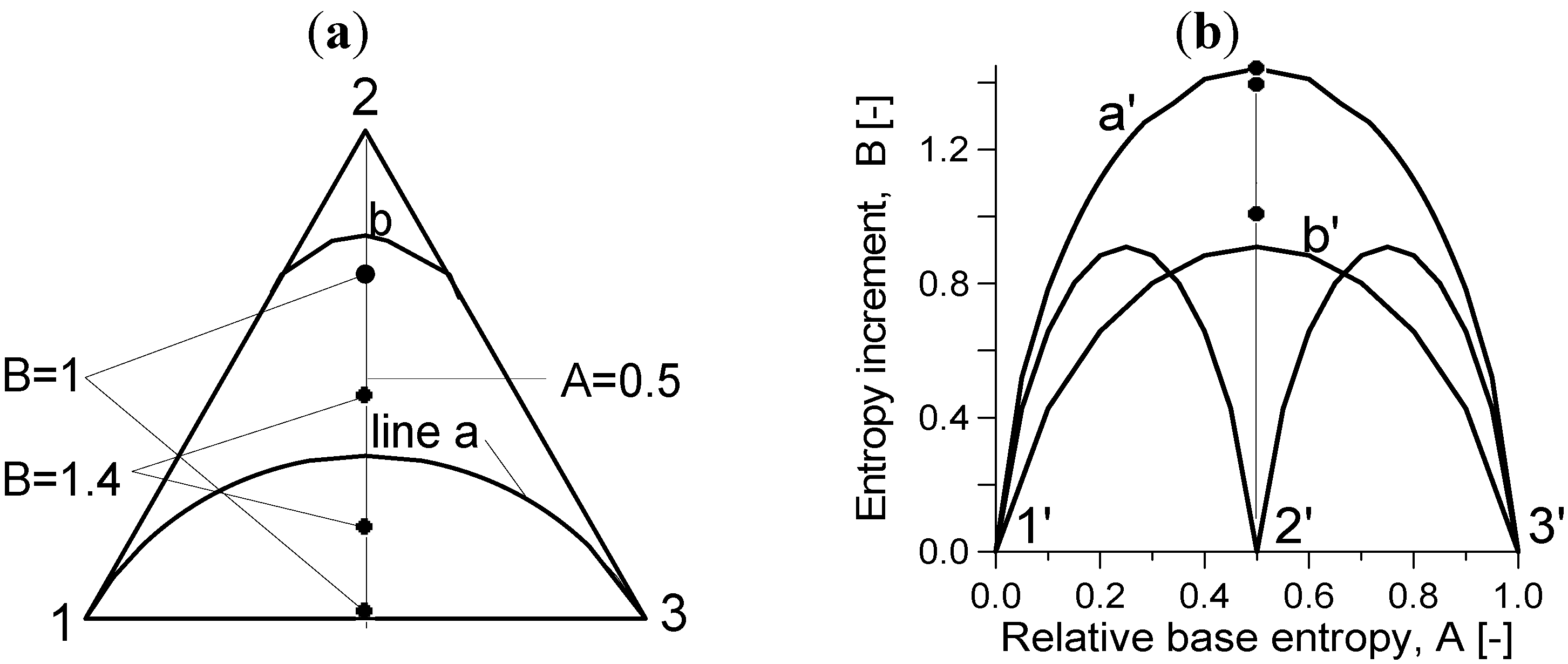Mapping between the normalized entropy diagram and its corresponding simplex for a soil with N = 3 fractions is illustrated in Figure 1.

Figure 1. Mapping between the normalized entropy diagram and its corresponding simplex for a soil with N = 3 fractions (a) The 2D simplex (N = 3) and its A = 0.5 hyper-plane section. (b) The normalized entropy diagram with points of A = 0.5, B = 1.4 and A = 0.5, B = 1.4. [The inverse images of these points in (ii) are shown in the A = 0.5 hyper-plane section of the 2D simplex in (i). The inverse image of line a' (the maximum B) in (ii) is line a in (i); the inverse image of the line b' in (ii) is line b in (i)].

Figure 1. Mapping between the normalized entropy diagram and its corresponding simplex for a soil with N = 3 fractions (a) The 2D simplex (N = 3) and its A = 0.5 hyper-plane section. (b) The normalized entropy diagram with points of A = 0.5, B = 1.4 and A = 0.5, B = 1.4. [The inverse images of these points in (ii) are shown in the A = 0.5 hyper-plane section of the 2D simplex in (i). The inverse image of line a' (the maximum B) in (ii) is line a in (i); the inverse image of the line b' in (ii) is line b in (i)].

2.4.1. Maximum and Minimum Entropy Increment Lines

A point of the maximum B line can be best computed by conditional optimization [4]. According to the solution, for a fixed number of fractions N and normalized base entropy A, the following grading curve maps into this point:

$$x_1=\frac{1}{{\displaystyle \sum _{j=1}^N{a}^{j-1}}}=\frac{1-a}{1-a^N}$$

(9)

$$x_j=x_1 a^{j-1}$$

(10)

where parameter a is the root of:

$$y={\displaystyle \sum _{j=1}^N{a}^{j-1}}[j-1-A(N-1)]=0$$

(11)

Following from Descartes rule of signs, polynomial y has one and only one positive root for a [15]. As A varies between 0 and 1, the positive root a varies between 0 and ∞, with the extreme values corresponding to the extreme fractions 1 and N [4]. These points of the simplex constitute a continuous line which can be seen in Figure 1a. The corresponding grading curves are the optimal grading curves shown in Figure 2.

The minimum bounding line has less significance than the maximum bounding line, and therefore generally, instead of the cumbersome determination of the precise conditional minimum, the image of edge 1 – N is used as an approximate minimum B (or ΔS) bounding line.

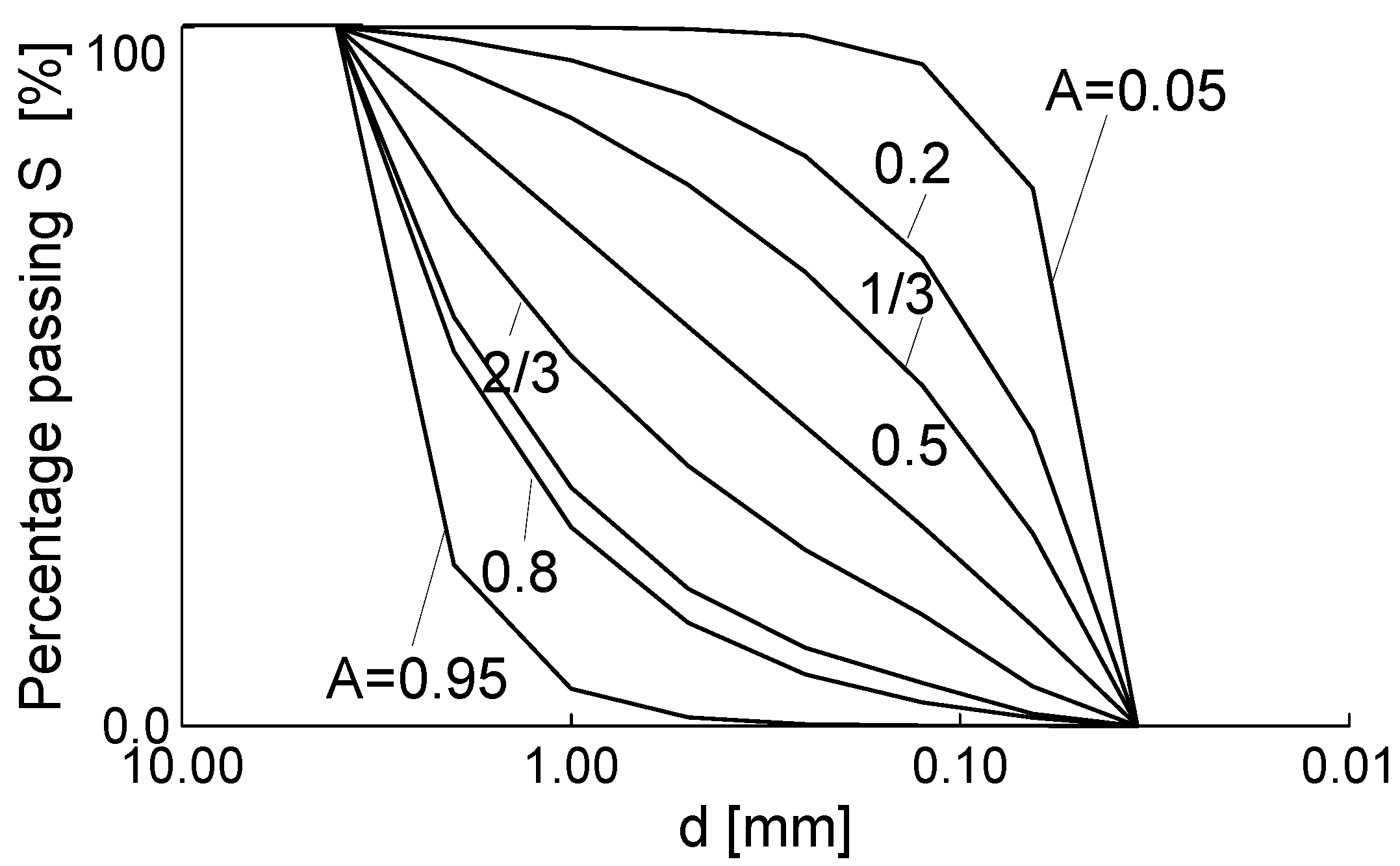
Figure 2. Optimal grading curves for N = 7; A varies. Note in this figure, that the grading curves with A < 0.5 are referred to as concave down curves, and the grading curves with A > 0.5 are referred to as convex down curves.

Figure 2. Optimal grading curves for N = 7; A varies. Note in this figure, that the grading curves with A < 0.5 are referred to as concave down curves, and the grading curves with A > 0.5 are referred to as convex down curves.

2.4.2. Multiple Diagram

In a multiple diagram, a finite number of simplexes (with various N and d_min values) can be represented through the entropy map, as shown in Figure 3. In the case of the multiple normalized entropy diagram, the range of the normalized coordinates and the location of the global maximum point of B are independent of N (B = 1/ln2). 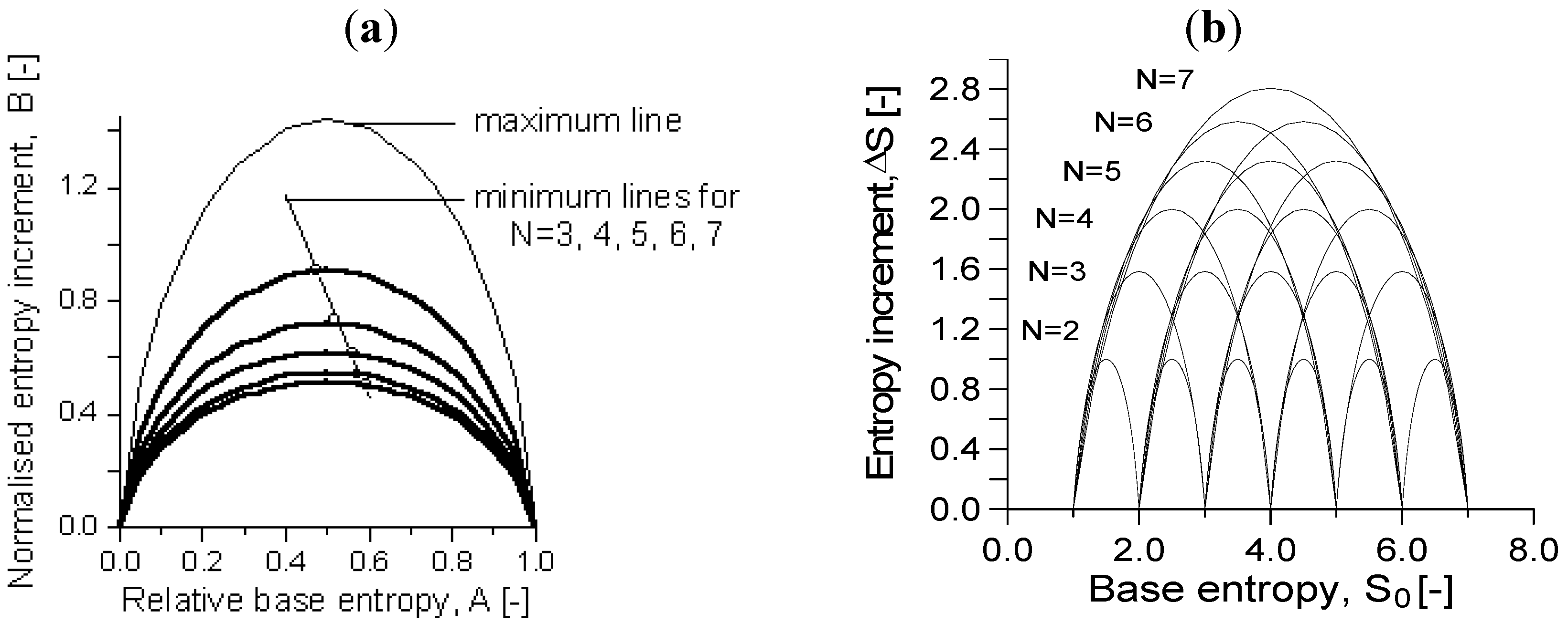For small N values, the maximum B lines nearly coincide with, and can be approximated to, the simple specific entropy formula that is valid for N = 2. In the case of the multiple non-normalized entropy diagram, the maximum value of the maximum ΔS lines is lnN/ln2 and the maximum value of the approximate minimum ΔS lines is 1.

Figure 3. The multiple diagram. (a) The normalized entropy map for simplexes with N varying from 2 to 7, the coinciding maximum B lines and the approximate minimum B lines. (b) The non-normalized entropy diagram (where the single and multiple diagrams are identical) for the continuous sub-simplexes of a simplex with N = 7 and the maximum ΔS lines.

Figure 3. The multiple diagram. (a) The normalized entropy map for simplexes with N varying from 2 to 7, the coinciding maximum B lines and the approximate minimum B lines. (b) The non-normalized entropy diagram (where the single and multiple diagrams are identical) for the continuous sub-simplexes of a simplex with N = 7 and the maximum ΔS lines.

2.4.3. Discontinuous Entropy Paths in the Normalized Diagram

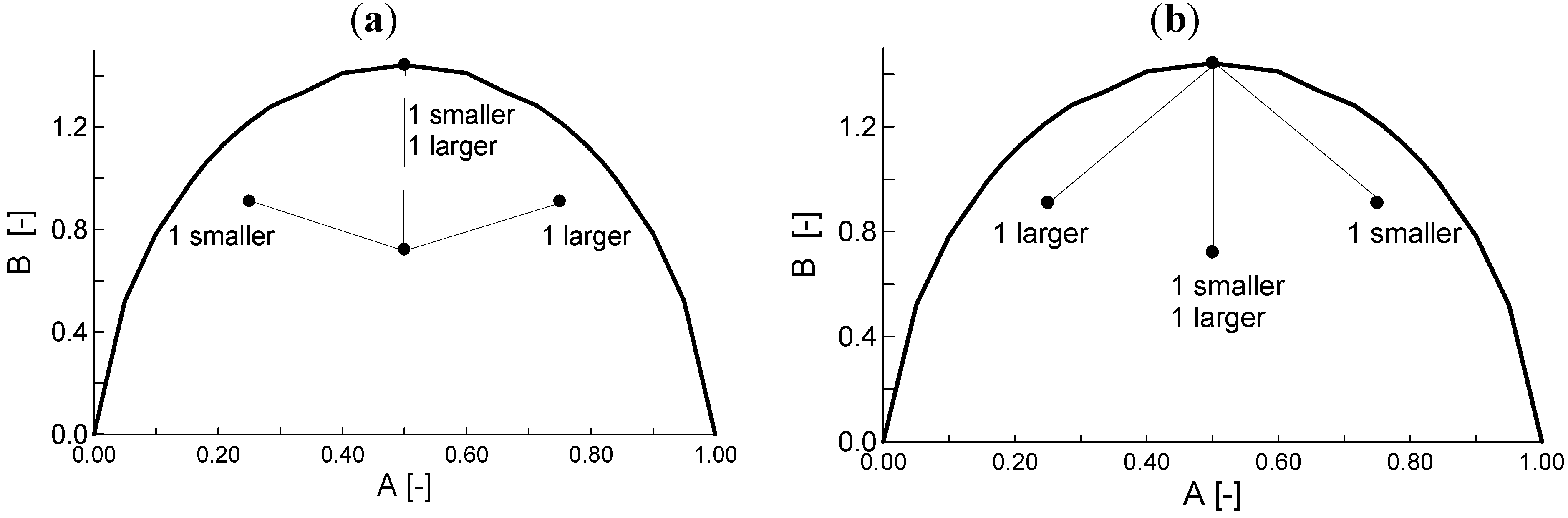
For soils undergoing changes in particle size distribution, the entropy coordinates move within the entropy diagram. Changes in the entropy coordinates do not only result from changes in the relative frequency x_i (i = 1, 2, 3, ..., N): it is also possible that new fractions can appear, or that existing fractions can be eliminated, thus changing N. Since the formulae of the normalized entropy coordinates contain parameter N, the normalized coordinates will be discontinuous if the integer variable N changes.

The discontinuity of the normalized entropy map with respect to the fraction number N is illustrated in a simple example here, and is analysed in detail by Lőrincz et al. [16]. Consider a two-fraction soil, with relative frequencies x₁ = x₂ = 0.5. It can be considered as a three fraction soil if a new, larger or smaller, “zero” fraction (i.e., a coarser or finer fraction with zero particle frequency) is added. Data describing this situation is presented in Table 2. If the value of N is increased from two to three, then the resulting jump in A is either an increase (the zero fraction is added from the smaller side) or a decrease (the zero relative frequency fraction is added to the larger side). These changes in the normalized entropy values are illustrated on diagrams in Figure 4. It can be noted, however, that if N changes by adding some zero fractions, the normalized entropy coordinates have a different value, but the non-normalized entropy coordinates remain the same.

Table 2. Illustration for the discontinuity of the normalized entropy path as a function of the zero fractions: various entropy coordinates for the ‘same’ actual collection of particles.

N [-]	2 (50% of grains in each fraction)	3 (smaller fraction added with zero frequency)	3 (larger fraction added with zero frequency)	4 (larger and smaller zero fractions added)
So min[-]	2	1	2	1
So max[-]	3	3	4	4
A [-]	0.5	0.75	0.25	0.5
B [-]	1/ln2	1/ln3	1/ln3	1/ln(4)

Table 2. Illustration for the discontinuity of the normalized entropy path as a function of the zero fractions: various entropy coordinates for the ‘same’ actual collection of particles.

N [-]	2 (50% of grains in each fraction)	3 (smaller fraction added with zero frequency)	3 (larger fraction added with zero frequency)	4 (larger and smaller zero fractions added)
So min[-]	2	1	2	1
So max[-]	3	3	4	4
A [-]	0.5	0.75	0.25	0.5
B [-]	1/ln2	1/ln3	1/ln3	1/ln(4)

Figure 4. Illustration for the discontinuity of the normalized entropy path as a function of the zero fractions: various entropy coordinates for the ‘same’ two-fractions, 0.5:0.5 grading curve. (a) taking away zero fractions; (b) adding zero fractions (see Table 2). Note that the jump is dependent not only the number of new zero fractions but also on the initial number of fractions.

Figure 4. Illustration for the discontinuity of the normalized entropy path as a function of the zero fractions: various entropy coordinates for the ‘same’ two-fractions, 0.5:0.5 grading curve. (a) taking away zero fractions; (b) adding zero fractions (see Table 2). Note that the jump is dependent not only the number of new zero fractions but also on the initial number of fractions.

3. Application of the Stability Criteria to Piping — Softening Soils

When water permeates a granular soil, it can either pass through the matrix of grains without affecting the relative grain arrangement (i.e., the grain structure is stable), or it can cause grains to be mobilized and rearranged. The basic types of the particle movements in structurally unstable granular assemblages are suffosion, erosion, piping, segregation and filtration (colmation) [17]. The prerequisites for the particle movement (structural instability) are as follows: (i) there is enough energy in the seepage water (suitable hydraulic conditions) to mobilize the particle, and (ii) there is a suitably situated pore channel for the particle to migrate (suitable geometrical conditions). The geometrical conditions are formulated below in terms of entropy criteria [2].

3.1. General Stability Criteria for Piping

Domains related to the stable/unstable behavior of grain structures have been successfully identified on the normalized entropy diagram, on the basis of simple permeameter tests undertaken by Lőrincz [1,2]. The criteria for grain structure stability or particle migration (suffosion, piping) were elaborated on the basis of vertical water flow tests (“wash-out tests”) where the soil was placed into a cylindrical permeameter (20 cm height and 10 cm diameter) bounded at the bottom by a sieve. The bottom meshes were chosen to permit the passage of particles smaller than 1.2 mm but retain particles larger than 1.2 mm. The applied downward hydraulic gradient, i, was as large as 4 or 5.

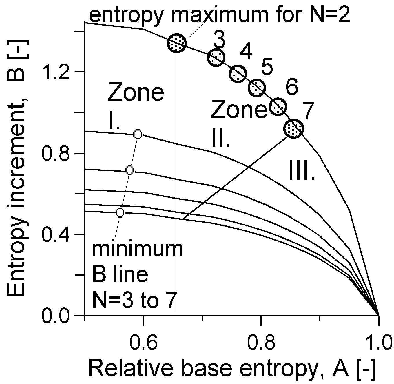
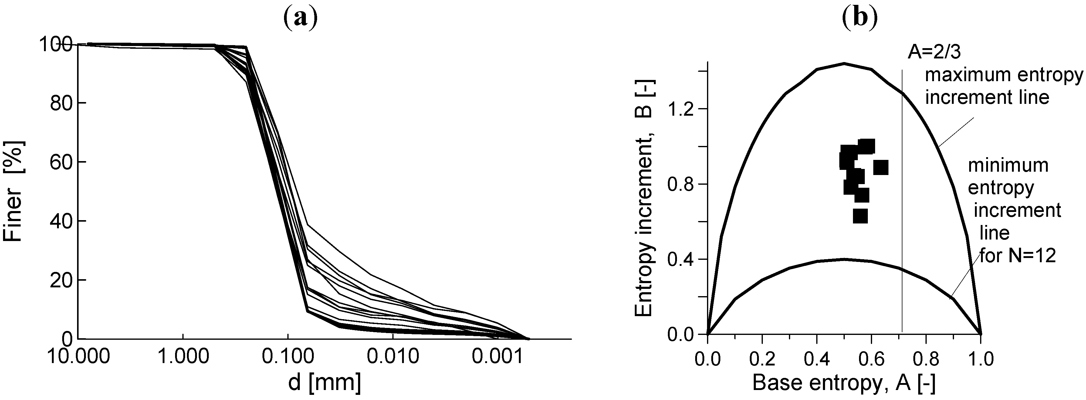
The soil structure stability zones identified are shown on the normalized entropy diagram in Figure 5 (note only the half of the symmetric diagram is shown). If A < 2/3 (Zone I), the structure of the large grains is unstable, smaller particles can be dislodged and erosion/piping may occur. This result can be interpreted as corresponding to a phenomenon where the coarser particles “float” in the matrix of the finer ones, and become destabilized when the finer particles are removed.

If A > 2/3 the coarser particles form a resistant skeleton and total erosion cannot occur. In Zone II, the structure of smaller and larger particles is inherently stable, and there are no particle movements: the larger particles retain the smaller particles, and the smaller particles support the larger ones. In Zone III, the fines may migrate in the presence of seepage flows (“suffosion”), but they are unable to cause collapse of the structural skeleton of coarser particles.

Figure 5. Particle migration zones in the simplified normalized diagram (I-piping. II-stable. III-stable with suffosion) and maximum entropy points.

Figure 5. Particle migration zones in the simplified normalized diagram (I-piping. II-stable. III-stable with suffosion) and maximum entropy points.

3.2. Piping and Softening Soil Case Studies in Dikes in Hungary

Underground erosion (piping) is one of the most frequent causes of failure in flood protection levees [8,18,19]. Soils prone to piping are difficult to identify from geotechnical testing data beforehand [20].

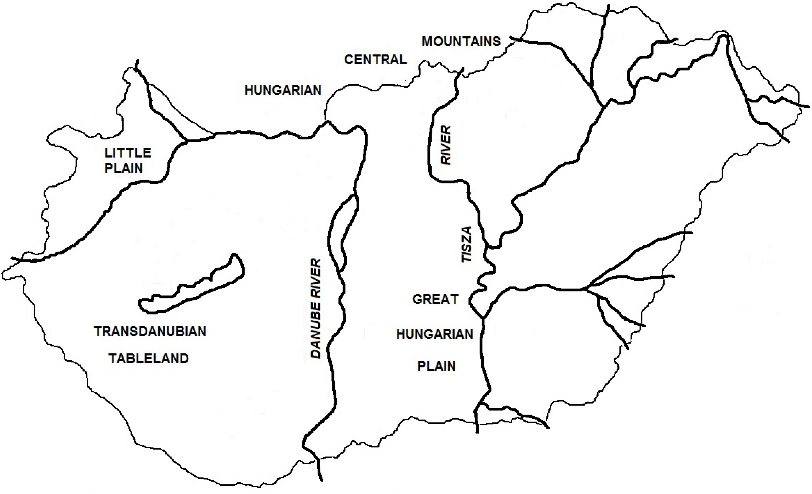
Hungary has the longest river dike system in Europe, adjacent to the rivers Danube and Tisza and their tributaries (e.g., Maros, Körös) as shown in Figure 6. The total volume of the dikes is about 170 million cubic meters. The Danube valley is covered by a 0.5–6.0 m thick layer of silty Quaternary sediment. The riverbed is formed in the underlying granular soils. Typically, dikes along the Danube are made from sandy material in the northern part and silty material in the southern areas. The subsoil of the Tisza-Körös valley varies from basically granular in the northern part, to highly plastic (clayey) in the southern part.

Figure 6. The rivers in Hungary.

Figure 6. The rivers in Hungary.

Dikes of the Danube have a typical height of about 6 to 8 m, with a crest width of 4 m. The riverside slope is 3:1, the landward slope is 2:1. The dikes have been built of silt (plasticity index 12–20%), sand or sandy gravel. Typical foundations under dikes comprise stratified sands and silts overlying highly permeable sandy gravel beds.

The dikes of the Tisza River are similar, although the height is generally less than 6 m. The earlier dikes were constructed with a riverside slope of 3:1 and a landward slope of 2:1, but later the slopes were modified in some places to 5:1. The Tisza dikes have been built of less permeable soils than in the case of the Danube banks, including Holocene silts and clays from adjacent to the river.

For dikes that are performing according to design, water normally appears on the outer face after about 10–12 days of the river rising (and in the case of repetitive floods, after 5–6 days). The amount of water is not qualitatively different for the different dike materials. The dikes usually “dry out” in a few sunny days after the river level subsides. For dikes that are not performing correctly, the water appears at the outer surface much earlier, indicating preferential flow paths. The most frequent mode of flood damage is piping, which generally occurs at the interface of natural and constructed layers. Piping in the dikes develops from the erosion of fine particles from a finer, unstable cover layer into a coarser, more permeable base layer.

Dike breaches can also be caused by softening, slides or surface erosion due to the localized presence of saline soils. These are less frequent, and only generally become apparent during the flood period.

3.2.1. Case Studies for Piping

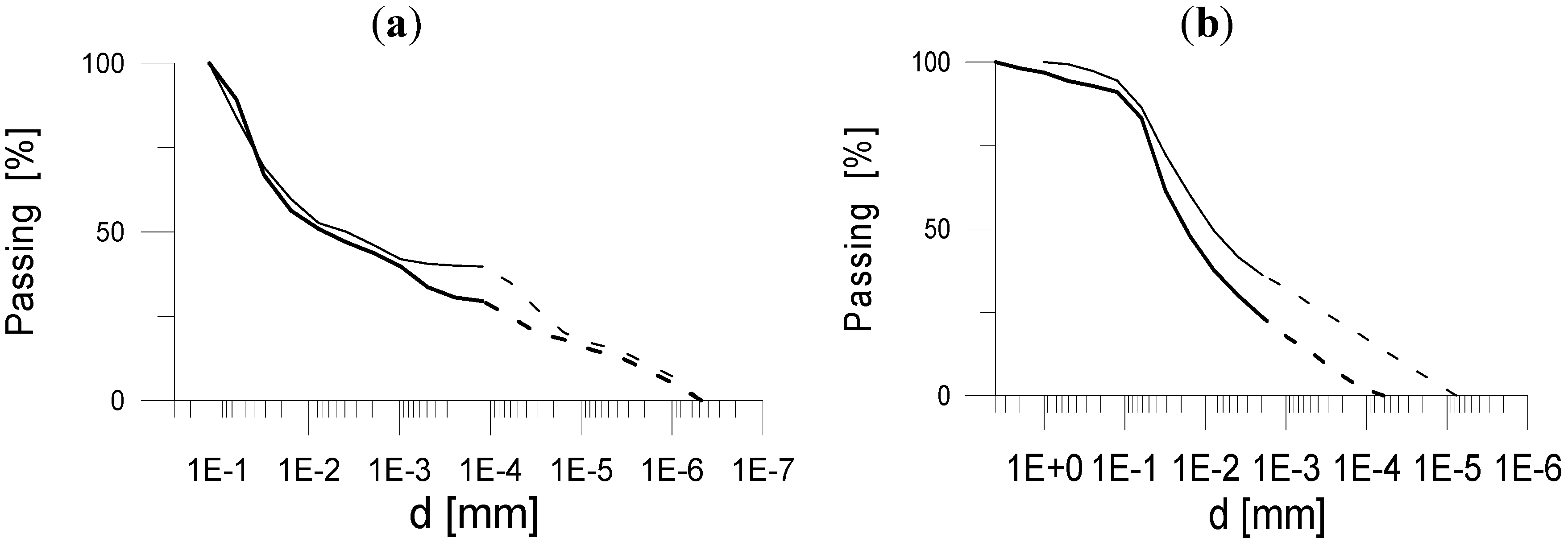
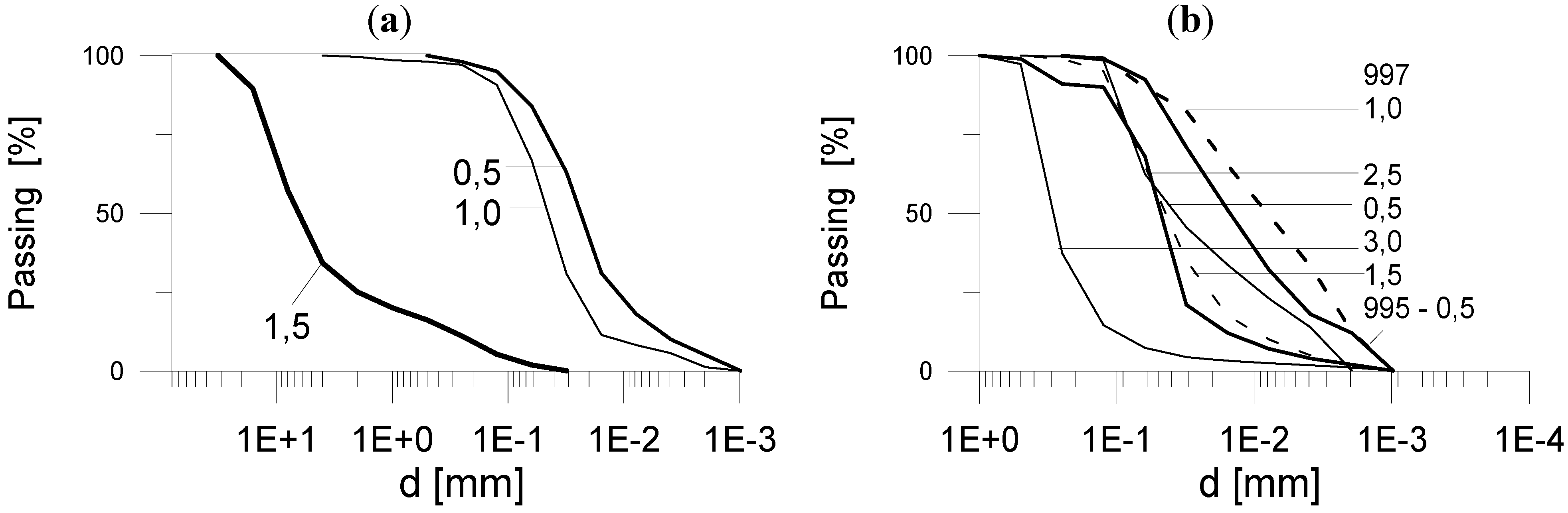
Studies of piping failures have been carried out for Hungarian dikes over many years, and there is a good body of data with which the grading entropy criteria can be compared. Piping was observed at several locations along the Danube River during the flood period of 1965. Piping took place in soil layers situated above sandy gravel beds. Soil layers below the dike were explored at two piping sites: at Dunakiliti and Dunafalva. These are summarised in Table 3. At Dunakiliti, the sequence comprised a 0.5 m thick silt layer and a 0.5 m thick “Mo” layer (non-plastic fine sand or “sand flour”) above the sandy gravel layer. At Dunafalva, the sequence comprised Mo, silt, Mo and fine sand layers with thicknesses of 0.6, 0.9, 1.3, 0.2 m respectively, above the sandy gravel bed. The grading curves are shown in Figure 7 and entropy values are given in Table 4.

The Dunakiliti and Dunafalva cases both involve finer, unstable cover layers over more permeable layers, which lead to arrangements that might be prone to piping. The Dunakiliti surface layers (0.5 m and 1 m) and the Dunafalva surface layer (0.5 m) have very similar particle size distribution curves. Similarly, below these erodible soils, much coarser and more permeable soils are encountered in the river bed: the Dunakiliti deeper layer (at 1.5 m) and the Dunafalva deeper layer (at 3.0 m) are also very similar to each other, and very different to the surface layers.

Figure 7. Grading curves for the Danube dike case studies. The numbers represent borehole numbers and depths with reference to Table 3. (a) Dunakiliti soils; (b) Dunafalva soils.

Figure 7. Grading curves for the Danube dike case studies. The numbers represent borehole numbers and depths with reference to Table 3. (a) Dunakiliti soils; (b) Dunafalva soils.

Table 3. Stratification of Danube dike soils.

Stratification at Dunakiliti (borehole 997)		Stratification at Dunafalva (borehole 993)
Soil type	Layer boundaries [m]	Soil type	Layer boundaries [m]
silt	0 to 0.5 m	Mo*	0 to 0.6 m
Mo*	0.5 to 1.0 m	silt	0.6 to 1.3 m
sandy gravel	below 1.0 m	Mo*	1.3 m to 2.2 m
		fine sand	2.2 m to 3.0 m
		sandy gravel	below 3.0 m

* Mo refers to a fine sand soil (0.02 mm and 0.1 mm), referred to locally as “sand flour” according to the Hungarian standard. It is a very frequent soil type in Hungary.

Table 3. Stratification of Danube dike soils.

Stratification at Dunakiliti (borehole 997)		Stratification at Dunafalva (borehole 993)
Soil type	Layer boundaries [m]	Soil type	Layer boundaries [m]
silt	0 to 0.5 m	Mo*	0 to 0.6 m
Mo*	0.5 to 1.0 m	silt	0.6 to 1.3 m
sandy gravel	below 1.0 m	Mo*	1.3 m to 2.2 m
		fine sand	2.2 m to 3.0 m
		sandy gravel	below 3.0 m

* Mo refers to a fine sand soil (0.02 mm and 0.1 mm), referred to locally as “sand flour” according to the Hungarian standard. It is a very frequent soil type in Hungary.

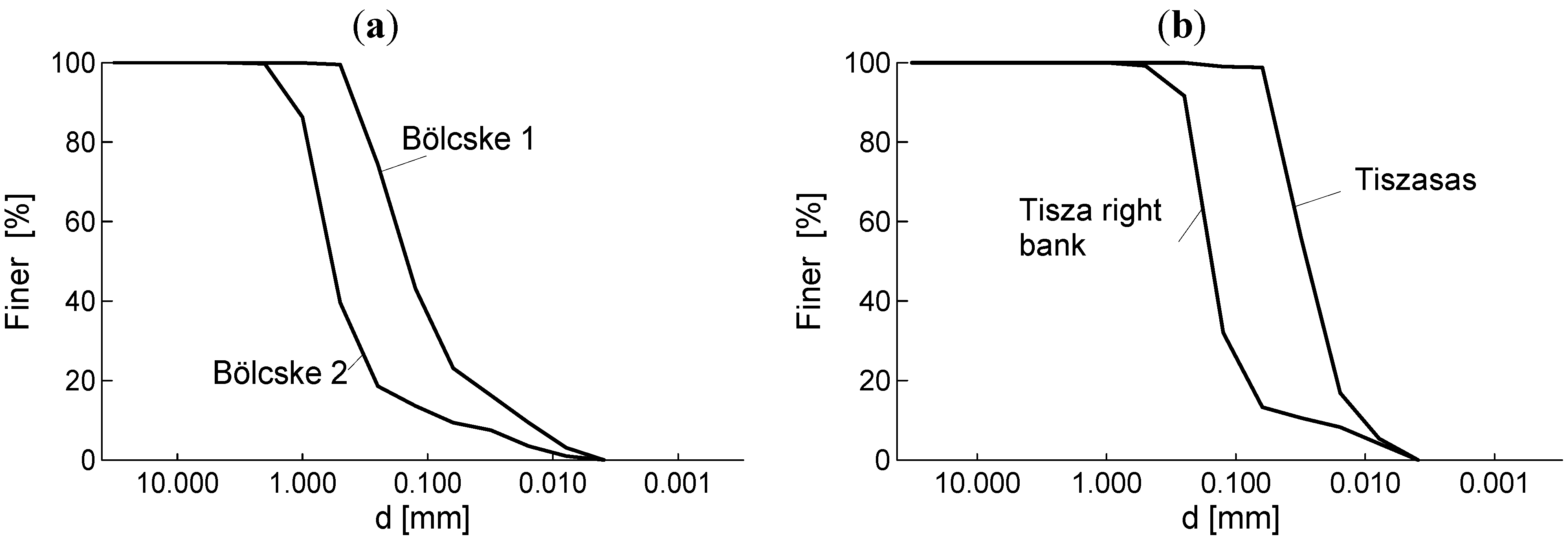
This data is augmented by more recent data, from sites where the wash-out materials from piping events at the Bölcske, Tiszasas and the Tisza right bank were sampled and characterised [21]. A total of 83 samples were assessed. Typical grading curves for these soils are shown in Figure 8 and entropy values are given in Table 4.

Figure 8. Washed-out materials from piping sites [21]. (a) Grading curves for a Danube site (Bölcske); (b) Grading curves for two Tisza sites (Tiszasas, Tisza right bank).

Figure 8. Washed-out materials from piping sites [21]. (a) Grading curves for a Danube site (Bölcske); (b) Grading curves for two Tisza sites (Tiszasas, Tisza right bank).

Table 4. Entropy data of piping soils at the Danube.

No of example	Site	Borehole	Depth [m]	N [-]	A [-]	B [-]
1	Dunakiliti	997	0.5	9	0.50	1.19
2	Dunakiliti	997	1.0	15	0.45	0.92
3	Dunakiliti	997	1.5	10	0.71 > 2/3	1.22
4	Dunafalva	993	0.5	8	0.46	1.01
5	Dunafalva	993	1.0	8	0.38	1.34
6	Dunafalva	993	1.5	9	0.59	1.05
7	Dunafalva	993	2.5	10	0.56	1.01
8	Dunafalva	993	3.0	10	0.81 > 2/3	0.78
9	Dunafalva	995	0.5	8	0.46	1.31
10	Bölcske 1	surface	surface	10	0.69 > 2/3	0.99
11	Bölcske2	surface	surface	9	0.54	1.12
12	Tiszasas	surface	surface	6	0.45	0.96
13	Tisza right bank	surface	surface	8	0.63	0.91

Table 4. Entropy data of piping soils at the Danube.

No of example	Site	Borehole	Depth [m]	N [-]	A [-]	B [-]
1	Dunakiliti	997	0.5	9	0.50	1.19
2	Dunakiliti	997	1.0	15	0.45	0.92
3	Dunakiliti	997	1.5	10	0.71 > 2/3	1.22
4	Dunafalva	993	0.5	8	0.46	1.01
5	Dunafalva	993	1.0	8	0.38	1.34
6	Dunafalva	993	1.5	9	0.59	1.05
7	Dunafalva	993	2.5	10	0.56	1.01
8	Dunafalva	993	3.0	10	0.81 > 2/3	0.78
9	Dunafalva	995	0.5	8	0.46	1.31
10	Bölcske 1	surface	surface	10	0.69 > 2/3	0.99
11	Bölcske2	surface	surface	9	0.54	1.12
12	Tiszasas	surface	surface	6	0.45	0.96
13	Tisza right bank	surface	surface	8	0.63	0.91

3.2.2. Case studies for Softening and Saline Soils in Hungary

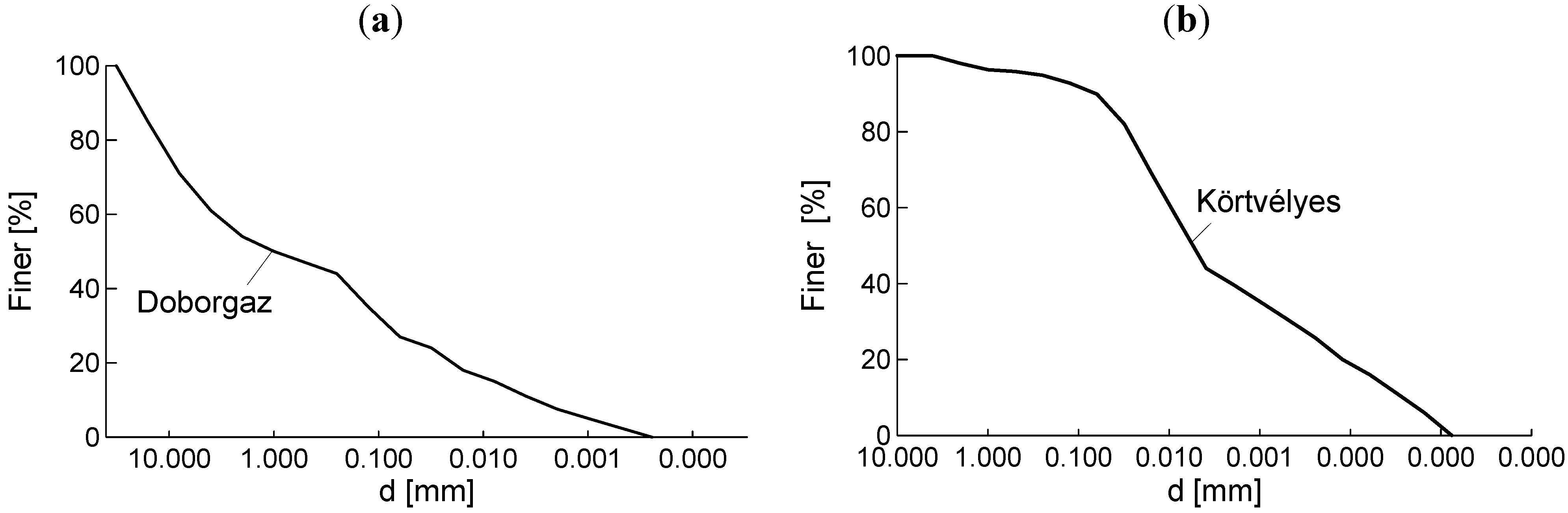
The presence of ‘softening’ or collapsing soils at the toe of natural slopes is also a recognized geotechnical issue [22] and this too is difficult to identify in soils in advance. Serious softening of the surface soil layer was observed along the Danube River during the flood period of 1965, within some meters from the toe of the dike. Soil samples were taken from the softening surface layer at a site near Doborgaz and characterised. The data is shown in Table 5 and the grading curves are shown in Figure 9. In another case, a sudden, complete fluidization of a part of the dike toe occurred due to the presence of a very saline soil in the surface layer beneath a dike beside the Tisza river in Körtvélyes in 1974 [23]. A sample of the saline surface layer was taken and characterised and the results are also shown in Table 5 and Figure 9.

Figure 9. Grading curves for case studies for surface softening. (a) Grading curves for a Danube site (Doborgaz); (b) Grading curves for three Tisza sites (Körtvélyes).

Figure 9. Grading curves for case studies for surface softening. (a) Grading curves for a Danube site (Doborgaz); (b) Grading curves for three Tisza sites (Körtvélyes).

Table 5. Entropy data of softening soils.

No of example	Site	Borehole	Depth [m]	N [-]	A [-]	B [-]
14	Doborgaz	surface	0.0	17	0.65	1.34
15	Körtvélyes	surface	0.0	15	0.42	1.29

Table 5. Entropy data of softening soils.

No of example	Site	Borehole	Depth [m]	N [-]	A [-]	B [-]
14	Doborgaz	surface	0.0	17	0.65	1.34
15	Körtvélyes	surface	0.0	15	0.42	1.29

3.3. Analysis of Results

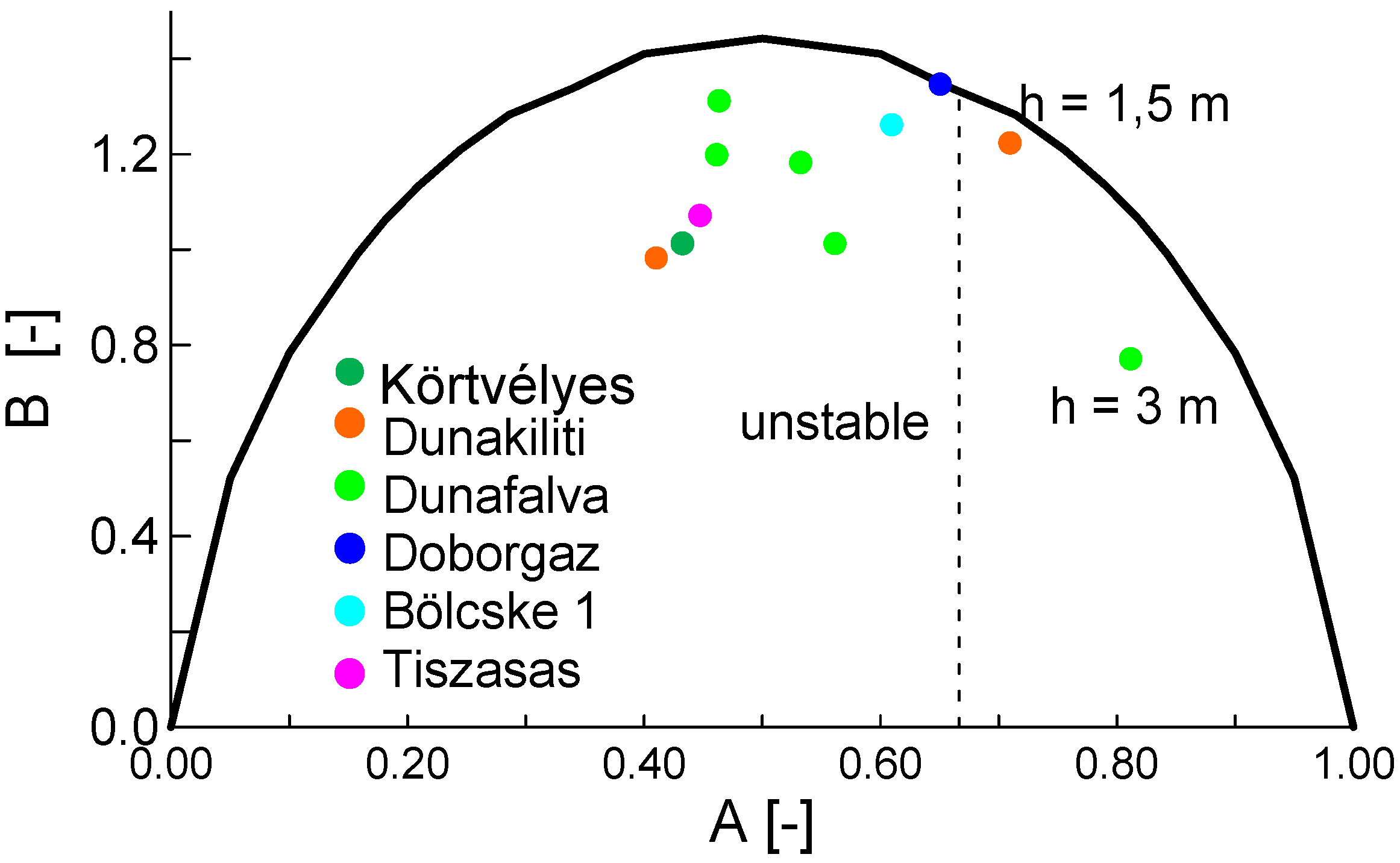
The normalized entropy data for the piping sites at Dunakiliti, Dunafalva, Bölcske, Tiszasas and the Tisza right bank are plotted with the entropy data from the softening soil sites at Doborgaz and Körtvélyes in Figure 10. It is apparent from Figure 10 that in all but two cases, the entropy data falls in Zone 1 of the plot, confirming the potential for these soils to be affected by piping behaviour. Only three of the 83 samples from Bölcske, Tiszasas and the Tisza right bank are shown on the plot, but Nagy [21] reports that of the 83 samples evaluated, 69 were found to be prone to piping, according to the criteria defined in terms of normalized grading entropy.

The fundamental behaviour in these cases involves migration and erosion of the finer particles, which in turn destabilises the coarser particles. Under the action of sustained seepage flows, cavities grow and propagate, causing the development of pipes. It is important to note that an assessment of the out-washed soils found them to be similar to the soils identified as unstable in Figure 7 and the soils shown in Figure 8. These are not silt, but rather they are more related to the category of Mo or “sand flour”, at the boundary between coarse silt and fine sand (0.02 mm to 0.1 mm). Mo has practically no cohesion and low friction angle in shear tests: that is, it has not only an unstable structure, but also extremely low shear strength.

It is noted that these washed out soils are prone to liquefaction according to the criterion of Smoltczyk [24], indicating that the causes of piping and liquefaction may be somehow related [25,26]. Szepessy [27] suggested that a “dynamic liquefaction” effect could possibly arise from micromechanical shear forces as seepage is initiated and the seepage nfront progresses through the soil. This area needs further research. It is reassuring, however, that using grading entropy criteria, these soils are reliably identified as potentially unstable.

The data for the “softening” soils of Doborgaz and Körtvélyes also plot amongst the piping soils data in Zone 1. As the cause of the softening effect is unclear, it is not certain whether it is actually related to piping, or whether a different effect is responsible.

In summary, whilst the grading curve information for the different soils shows great variability, and identification of piping behaviour would be difficult, the examples presented show that normalized grading entropy provides a relatively reliable tool for predicting piping potential in a variety of soil types.

Figure 10. Normalized entropy data for the piping and softening soils from the Danube and Tisza river sites.

Figure 10. Normalized entropy data for the piping and softening soils from the Danube and Tisza river sites.

4. Grading Entropy-Based Criteria Applied to Dispersive Soils

4.1. General Stability Criteria for Dispersion

Dispersion is a behavior exhibited by particular clay minerals such as sodium montmorillonite. In the presence of saline pore water, grains of such clays experience collapse of their diffuse double layers (DDLs), allowing them to aggregate through intergranular attractions developed at close range [28]. This gives the clays an apparent cohesion. When these clays are then exposed to less saline water, salt in the pores is flushed out, allowing the DDLs to expand, overcoming their mutual attraction (apparent cohesion) and allowing them to be eroded. Whilst dispersion is strictly a surface phenomenon, loss of grains from the surface exposes the soil at deeper levels, consequently allowing it to disperse. If not arrested, this becomes a perpetuating process causing cavities to form and propagate to form pipes. Hence, dispersion of the clay grains in clayey silts may ultimately lead to piping. Accordingly, the criteria defined by Zone 1 in Figure 5 will also be applicable to dispersive clayey silt and silty clay soils.

A range of basic laboratory tests are suggested for the identification of dispersive soils, including: the pinhole test, analysis of the dissolved salts in the pore water, SCS dispersion tests, and crumb tests (see e.g., [29,30,31,32,33]). However, in many cases these criteria fail to categorize these soils reliably.

4.2. Examples for Dispersive Soils at Dams

Clay dams constructed from silty clay may fail at the first rise of the water level due to internal erosion facilitated by soil particle dispersion. As with piping soils, it is also difficult to identify dispersive soils in advance [33,34,35].

4.2.1. Wadi Quattarah Dam Case Study

The secondary dam of Wadi Quattarah (Libya) was built for irrigation water impoundment and flood control [36]. The dam consisted of a silty clay core, an inclined chimney drain, a blanket filter and a toe drain. The grading curves of the silty clay core are shown in Figure 11a. A trench was excavated to bedrock and back-filled with earth to form a cut-off. The maximum height was 28.0 m.

The dam failed at the first rise of the reservoir level when dispersion and piping took place in the silty clay core. The results of laboratory tests to confirm its dispersive nature were somewhat inconclusive: chemical analysis of the pore water showed that soil was moderately dispersive; the Crumb test gave similar results, but the pinhole test proved negative.

4.2.2. Los Esteros Dam Case Study

The Los Esteros dam (New Mexico) was also built for irrigation and flood water impoundment [37]. The grading curves are shown in Figure 11b. The dam consisted of an impervious core, rolled rock-fill upstream, a chimney drain on the downstream face of the core and downstream fill. It was founded on sandstone and shale. Its maximum height was 67 m.

Figure 11. Grading curves for the dispersive soils from the Wadi Quattarah and Los Esteros dam sites. (a) Wadi Quattarah dam; (b) Los Esteros dam.

Figure 11. Grading curves for the dispersive soils from the Wadi Quattarah and Los Esteros dam sites. (a) Wadi Quattarah dam; (b) Los Esteros dam.

Results of the first dispersivity tests were inconclusive. The pinhole test and the pore water chemistry indicated that soils were dispersive, but the crumb tests indicated that soils were non-dispersive. In the early stage of the construction, observations confirmed that the clay material to be used for the impervious core was, in fact, dispersive. Preventive measures were adopted including lime modification of the fractured foundation and application of a sand filter in chimney drain.

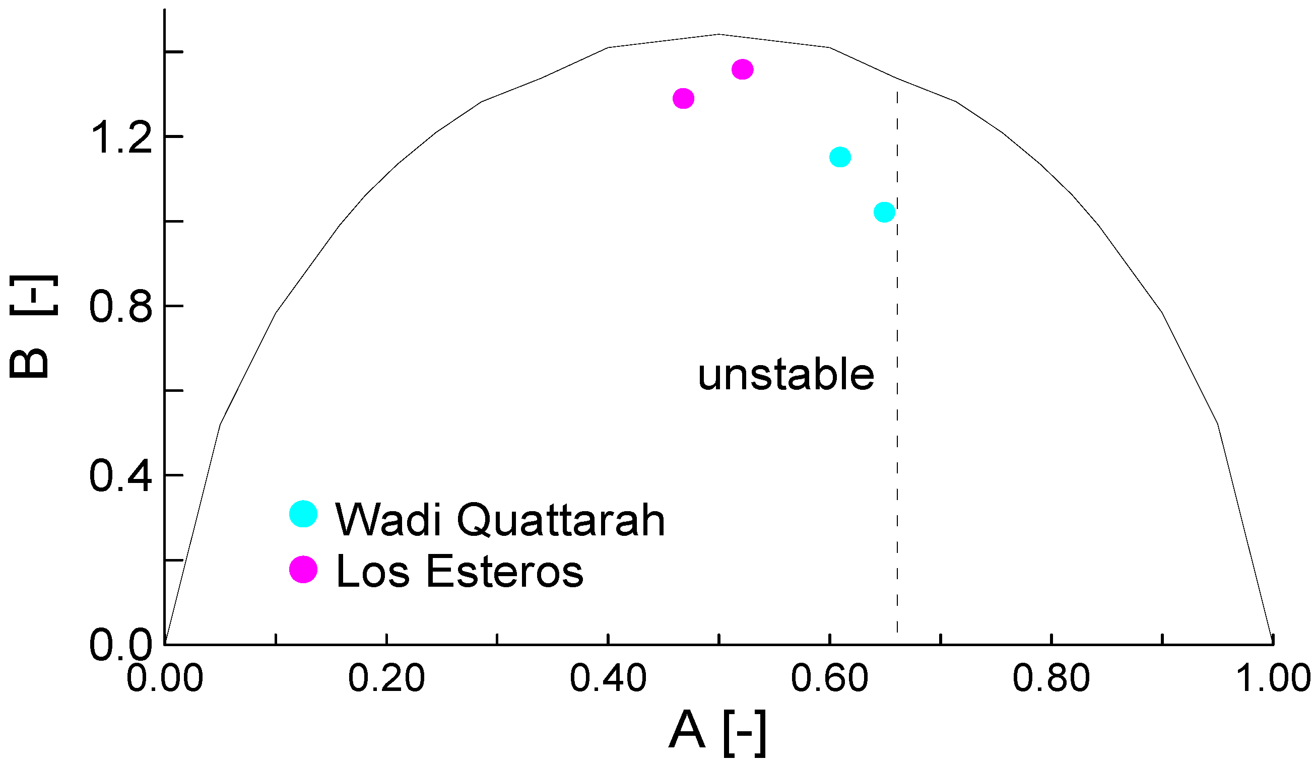
4.3. Analysis of Results

The normalized grading entropy values for the Wadi Quattarah and Los Esteros soils are presented in Figure 12 and Table 6.

Figure 12. Normalized entropy data for the Wadi Quattarah and Los Esteros dam sites.

Figure 12. Normalized entropy data for the Wadi Quattarah and Los Esteros dam sites.

Table 6. Entropy data of dispersive soils from the Wadi Quattarah and Los Esteros dam sites.

No of example	Site	N	A	B	Envelope
16	Los Esteros	16	0.47	1.29	lower
17	Los Esteros	17	0.52	1.36	upper
18	Wadi Quattarah	18	0.65	1.02	lower
19	Wadi Quattarah	18	0.61	1.15	upper

Table 6. Entropy data of dispersive soils from the Wadi Quattarah and Los Esteros dam sites.

No of example	Site	N	A	B	Envelope
16	Los Esteros	16	0.47	1.29	lower
17	Los Esteros	17	0.52	1.36	upper
18	Wadi Quattarah	18	0.65	1.02	lower
19	Wadi Quattarah	18	0.61	1.15	upper

The soils used in these two dams plot in the unstable Zone 1, which suggests that they are prone to piping. Although the soils were strictly dispersive, the ultimate failure is one of piping, wherein loss of clayey fines through dispersion becomes self-perpetuating in specific areas, causing cavities to form and propagate to form pipes. Hence, their identification as piping soils according to the criteria of Figure 5 is not inappropriate.

5. Grading Entropy-Based Criteria Applied to Filtering

5.1. Filtering Rule

A filtering rule was elaborated by Lőrincz [1] partly on the basis of the tests of Sherard [29] and partly on the basis of the suffosion tests of Lőrincz [1], which were interpreted from the self-filtering theory of [38]. It was formulated by cutting the gap-graded grading curves into two parts at the position of the gap and considering the coarse part as the filter and the fine part as the material being filtered (referred to as the base soil).

The difference between the filter and the base soil can be expressed using the entropy coordinates since these are pseudo-metrics [15] and specifically, the difference of the base entropies (S_of − S_ob: subscripts f and b denote the filtering layer and the base soil, respectively) is used for this purpose. However, since a certain value of S_o may belong to a fraction as well as to a widely graded soil, the ΔS entropy increments of both the filter and the base soils are included in the empirical relationship as their sum, ΔS_f + ΔS_b. 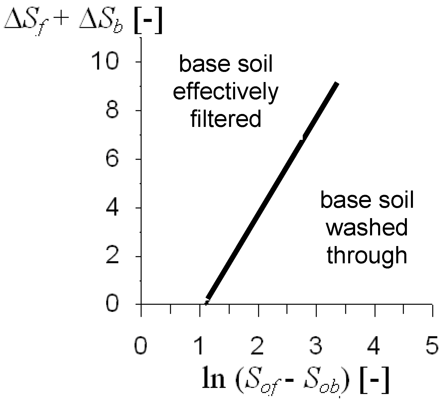Higher ΔS values imply broader grading curves. The empirical rule derived states that a granular layer acts as a filter for an adjacent layer of the base soil if the following condition is met in terms of entropy coordinates:

$$\Delta S_f+\Delta S_b\ge 4\ln (S_{0f}-S_{0b})-4.39$$

(12)

The domains defined by Equation (12) are shown in Figure 13.

Figure 13. The filtering criterion in the entropy diagram.

Figure 13. The filtering criterion in the entropy diagram.

where D and d refer to grain diameters in the filter and the base soil. Equation (13) corresponds to a situation where there are two empty size fractions between the filtering fraction and the filtered fraction. Exactly the same situation is incorporated in Equation (12): in the case when the filter and the base soil are single fractions, the left hand side is zero and S_of − S_ob is equal to 3, which means that two empty size fractions are between the filter and the base soil. In other words, the constant in Equation (12) was determined using this condition.

The application of grading entropy quantities helps in unifying the filtration rules. Testing against the foregoing general filter rule [1,3], it was found that Terzaghi’s filter rule [12,39] is generally too conservative. The same applies for Bertram’s rule and the rule recommended by the U.S. Bureau of Reclamation (USBR) [40] for uniform filters. Conversely, the mixed filter rule of the USBR is not conservative. It has to be noted that the same criterion seems to be valid for filtration of silty-clayey soils. Due to the lack of experimental results, the field of filtration needs further research.

5.2. Case Study at Kétpó Landfill

The leachate collection systems of landfills are generally built of granular soil: gravel and sand [41]. In some countries it is a requirement that the free surface of leachate remains within the drainage layer, at the base of the landfill. In general, a gravel layer is used. However, when biodegradation is expected to be significant in the landfill, sometimes biofilm leachate collection systems are used, which consist of several layers of various granular soils. In these leachate collection systems, some particle migration phenomena may occur if geotextile filters are not placed between the various granular layers [42,43].

A case study is presented here of a new leachate collection system where two granular layers were constructed in contact. The finer soil in the upper layer not only had an unstable structure but also, it was not filtered by the coarser soil below it. The system was installed for new landfill site in Kétpó, Hungary. Fine sand, 25 cm thick, was used as a drainage layer. The leachate collection tubes were covered by 5 cm of 16/32 inch gravel (S_o = 16, ΔS = 0) without an appropriate filter separator from the sand drainage layer. The grading curve of the fine sand is shown in Figure 14. The slope of the leachate collection system was 0.5% in both directions.

Investigations were made at the end of the construction. Sand and gravel were tested on the basis of grading entropy criteria to assess grain structure stability and filtering. The grading curves and corresponding grading entropy data for samples of the sand drainage layer are shown in Figure 14.

5.3. Analysis of Results

According to the grading entropy criteria (Figure 5) and the filtering rule (Figure 13), the sand has an unstable structure (Figure 14b) and is prone to be washed into the gravel (Figure 15: S_o = 7.8, ΔS = 2.55). This result was confirmed by observations of sand migration and loss after some heavy rainfall which also occurred immediately after the construction. A new drainage layer was planned on the basis of some simulations using the grading entropy-based criterion, which showed that if the fine material suffosed into the coarser layer, the free surface of the leachate may reach the bottom surface of the landfill in as little as a day.

Figure 14. Kétpó drainage sand layer. (a) Grading curves; (b) Grading curves in the normalized entropy diagram.

Figure 14. Kétpó drainage sand layer. (a) Grading curves; (b) Grading curves in the normalized entropy diagram.

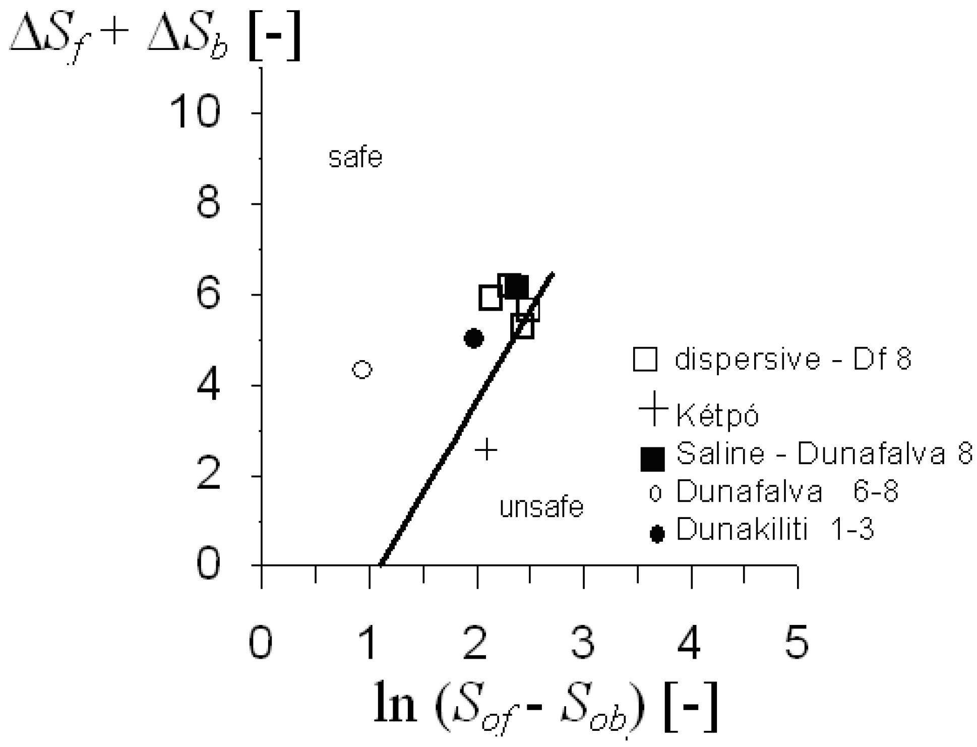
As a comparison, the soils described in the piping and dispersive soil case studies from the previous section were tested using the filtering criterion, to consider the possibility that the finer soils were being washed into the coarser river bed soils. The entropy data according to Equation (12) are plotted in Figure 15. Unlike the data for Kétpó, the soils from the Danube and Tisza dikes, and the Wadi Quattarah and Los Esteros dams were not found to be prone to losing fines into adjacent coarse grained layers. This result is consistent with observations that piping occurred within the soil layers themselves.

Figure 15. The grading curves in the filtering criterion entropy diagram.

Figure 15. The grading curves in the filtering criterion entropy diagram.

6. Grading Entropy Concept Applied to Particle Size Evolution

6.1. Particle Size Evolution

Although particle size evolution does not constitute the primary subject of this paper, it is considered briefly here to show that the concept of grading entropy can be applied to wider considerations than soil structure stability. As particle assemblages in either natural or engineered systems are modified, such as through particle breakage or aggregation, their corresponding grading entropy changes [4]. The directional properties of the variation of the grading due to particle breakage or aggregation can be described by changes in their grading entropy coordinates and related to the entropy principle [16]. The non-normalized entropy path during particle breakage is characterized by a monotonic increase in the entropy increment ΔS (entropy principle) and a decrease in the base entropy S_o (due to the decrease in the mean grain diameter). However, there is a discontinuity in the entropy path if the number of fractions increases due to the appearance of smaller fractions. In this situation, the discontinuity has an ‘opposite sign’ (the normalized base entropy A increases and the normalized entropy increment B decreases). These concepts can be extended to characterize the variation of grading curves during aggradation processes such as lime modification.

6.2. Lime Modification Test Results

In the process of lime modification, lime is added to a clayey soil in order to modify its physical properties such as plasticity, shear strength, durability, the freezing-thawing behaviour, etc. [44]. This occurs by causing a change in the clay crystal layer spacing, allowing to clay particles to rearrange and form new grain aggregates [45]. As a consequence, the apparent grading of the soil is modified, mostly through the aggregation of smaller particles to form larger ones.

The base entropy S_o, the weighted mean of the fraction entropies, is monotonically and uniquely related to the mean grain size and it follows that an increase in the mean grain diameter should cause an increase in S_o. The entropy increment ΔS is a measure of the disorder of the grain system, which originates from the mixing of the fractions. It can be related to the entropy principle. The normalized entropy path has the same behavior provided the number of fractions remains constant, as discussed in Section 2.4.3. However, it has a discontinuity if the number of fractions changes. In the situation of lime modification, the discontinuity has an ‘opposite sign’ to that which occurs during breakage (A decreases and B decreases) as smaller fractions tend to disappear.

Trang et al. [46] has been researching the effects of lime modification on grading at the Budapest University of Technology and Economics since 2004. The soils were prepared with various lime and water contents. The grading curve was determined at each stage of lime content increment. The results are presented here through three examples. Gradings (pre-modification) for two clays (Bánokszentgyörgy and Szarvas) and a loess (Adony) are shown in Table 7.

Table 7. Lime tested soils—classification test results for the unmodified soils.

Soil Fraction	Adony	Szarvas	Bánokszentgyörgy
Clay [%]	7.0	34.5	25.2
Silt [%]	55.6	52.7	62.6
Sand [%]	29.5	3.9	12.2
Gravel [%]	7.9	8.9	0.0
IP [%]	6.4	24.8	29.1

Table 7. Lime tested soils—classification test results for the unmodified soils.

Soil Fraction	Adony	Szarvas	Bánokszentgyörgy
Clay [%]	7.0	34.5	25.2
Silt [%]	55.6	52.7	62.6
Sand [%]	29.5	3.9	12.2
Gravel [%]	7.9	8.9	0.0
IP [%]	6.4	24.8	29.1

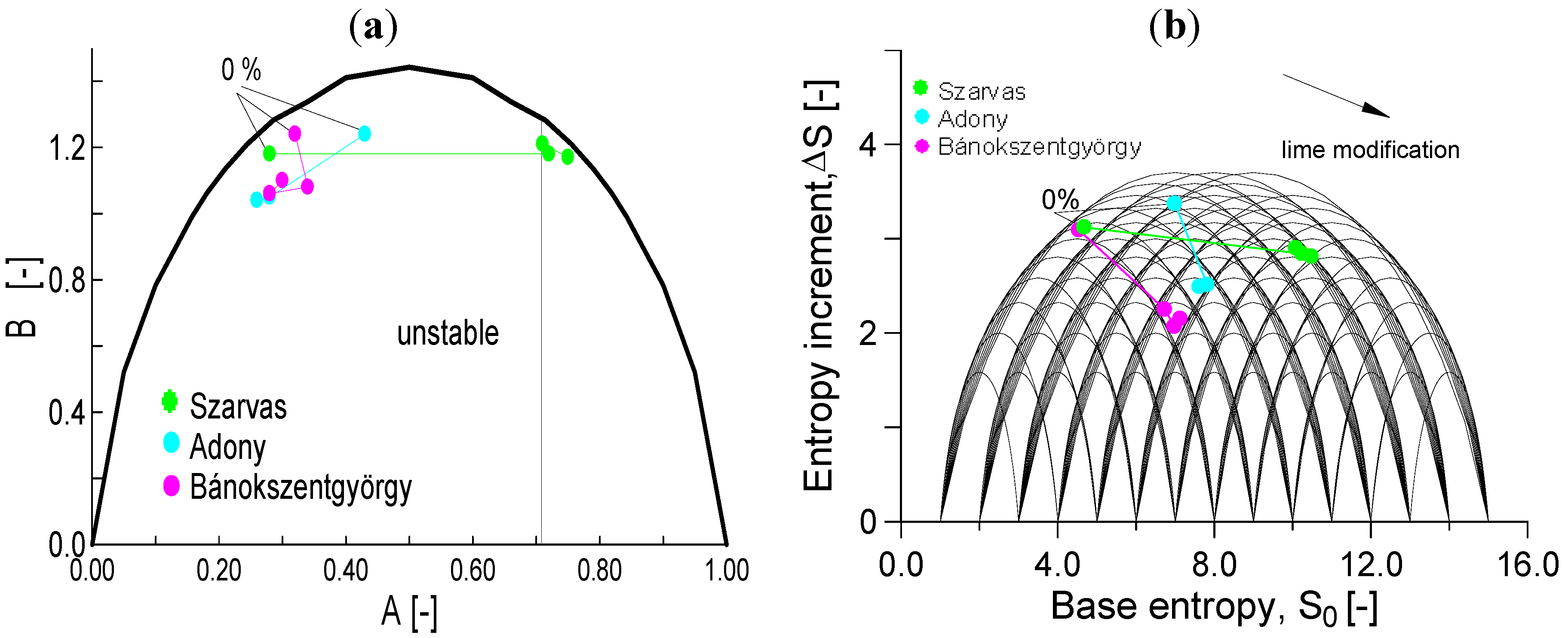
Figure 16a shows the normalized entropy paths for the three lime tested soils. After a few percent of lime, there was little evolution in the grading of the Adony and Bánokszentgyörgy soils, as reflected by the path of their normalized entropy coordinates. Neither soil shows any clear trends in entropy evolution: they are indeterminate in terms of A. They remained in the same region of the normalized entropy diagram (A < 0.5). On the contrary, for the Sarvas soil the grading curves did change significantly with the first addition of lime, causing the normalized base entropy to shift far to the right, and into Zone 2. This suggests that in the case of the Sarvas soil, lime modification was able to change the soil structure from an unstable arrangement to a stable arrangement, making it resistant to dispersion-induced piping (i.e., increasing the lime increases the aggregation, causing the number of fractions to decrease, and the smaller particles to disappear). It might be expected that the differing responses to lime might be due to variations in the plasticity of the different soils. However, such a trend is inconsistent, since only one of the two higher plasticity soils (Szarvas and Bánokszentgyörgy) demonstrated a significant effect.

However, the trends in the non-normalized entropy paths in Figure 16b are clearer: in all cases the base entropy only increases, the entropy increment only decreases and the soil tends to a more uniform grading. The base entropy increase is generally larger as the clay becomes more plastic.

Figure 16. Entropy paths of soils during lime modification. (a) In the normalized diagram (note that only the Szarvas soil becames stable). (b) In the non-normalized diagram.

Figure 16. Entropy paths of soils during lime modification. (a) In the normalized diagram (note that only the Szarvas soil becames stable). (b) In the non-normalized diagram.

6.3. Comparing Breakage and Lime Modification Test Results

The directional properties of the grading curve variation due to particle breakage (degradation) are connected to the grading entropy through the entropy principle. The non-normalized entropy path during breakage is characterized by a monotonic increase in the entropy increment ΔS (according to the entropy principle) and a decrease in the base entropy S_o (due to the decrease in the mean grain diameter). However, the entropy path will be discontinuous if the number of fractions increases due to the appearance of smaller fractions which increases the stability number A of the soil.

Lime modification produces an overall state improvement in terms of non-normalized entropy coordinates, and the change is opposite in direction to the case of breakage (or degradation) in terms of the non-normalized coordinates (S_o increases; ΔS decreases). The path in terms of normalized entropy coordinates is the basically the same except it is discontinuous when the number of fractions changes. One could expect that lime modified soils should become more stable in terms of their structure (i.e., A > 2/3). However, given the inconsistency of the effect of lime on the normalized base entropy A, the study indicates that the lime modification is not necessary helpful in improving stability.

7. Conclusions

The concept of grading entropy offers a new approach to some difficult practical problems in geomechanics, which are made more difficult because of the wide variability across particle size distributions. It can be applied successfully to predict undesirable soil phenomena such as dispersion, suffosion and piping. However, the application of the grading entropy principle is potentially useful far beyond these considerations, and particularly, it has the potential to increase our understanding of particle size evolution in natural and engineered systems. The case studies presented here illustrate this.

The normalized base entropy and entropy increment can be used as coordinates to define domains where different types of grain structure stability (or instability) prevail. The examined case studies support the hypothesis that particle migration criteria can be used to identify not only piping, but also dispersion and softening in cohesive soils, and filtering chsaracteristics in granular soils. In particular, susceptibility to piping failure can be reliably identified, as was demonstrated for silty sands (such as in the silty Hungarian dikes) where erosion of silt destabilises the coarser grains. The same criteria seem not only able to identify piping in granular soils, but also instability in dispersive soils and saline soils which are generally cohesive soils, but with a slight plasticity. It follows that the theory is likely to be valid for higher plasticity soils as well, however, further research is needed on this point since the inter-particle forces may have an important role.

It seems that the smallest fraction defined by Lőrincz [1] may not be small enough in the sense that the diameter of some dispersive clay grains may be less than the lower grain diameter limit of the smallest fraction (i.e., smaller than the width of elementary cell). However, it is noted that if the elementary cell width were decreased, the particle migration criteria would not change: the entropy increment ΔS would not change and the relative base entropy would simply be shifted by a constant.

The filtering rule can be reliably applied to evaluate situations in which coarse soils are meant to act as filters for adjacent finer soils, where there is a likelihood that the fine grains may be washed through. In the case study of the two-layer leachate collection system of the municipal landfill site, not only was the finer soil inherently unstable (on the basis of the stability criterion) but also, it was not filtered by the coarser soil (on the basis of the general filtering rule). Hence, the grading entropy criteria could be used to show that the design was completely unacceptable.

This study shows that the effect of lime modification on the grading curve evolution in the non-normalized grading entropy diagram is basically opposite to the effect of the usual particle breakage. Both can be related to the “entropy principle”. In the normalized grading entropy diagram, the grading curve evolution path is the same except that a discontinuity occurs at changes in the fraction number. The discontinuity can be quantified using the entropy coordinate A as stability measure (i.e., the stability increases with A). The discontinuity always leads to more stable structure for breakage but lime-induced aggregation may or may not increase the stability of the soil structure.