Deterministic Thermal Reservoirs

Abstract

We explore the consequences of a deterministic microscopic thermostat-reservoir contact mechanism for hard disks where the collision rule at the boundary is modified. Numerical evidence and theoretical argument is given that suggests that an energy balance is achieved for a system of hard disks in contact with two reservoirs at equal temperatures. This system however produces entropy near the the system-reservoir boundaries and this entropy flows into the two reservoirs. Thus rather than producing an equilibrium state, the system is at a steady state with a steady entropy flow without any associated energy flux. The microscopic mechanisms associated with energy and entropy fluxes for this system are examined in detail.

1. Introduction

The first concept established in equilibrium statistical mechanics is the existence of an equilibrium state; that is, after a sufficient time macroscopic observables have steady time independent average values. The concepts of temperature and entropy as applied in equilibrium thermodynamics cannot apply to some transient system and they do not easily generalize to nonequilibrium systems. However, it is possible that nonequilibrium steady states may have a thermodynamic description, particularly those that are close to equilibrium. For an isolated equilibrium system where the entropy is a maximum, if the system is connected to one or more reservoirs and perturbed from equilibrium the system is said to produce entropy. The entropy production is transferred to a reservoir or surroundings and the intrinsic entropy of the nonequilibrium system is lower than at equilibrium. Thus, when the perturbation is removed, the relaxation is driven by an increase in the intrinsic entropy. Perhaps a more useful construct is to instead consider the entropy flow as a flow of energy through the system that maintains it in a steady state. This energy flow has been called the housekeeping heat [1] to distinguish it from other intrinsic heat flows.

In the canonical ensemble a system is in thermal contact with a reservoir which can exchange energy with the system but is sufficiently large so that its thermodynamic state is not effected. Here it is assumed that the system comes to an equilibrium state and the details of the thermal contact are not believed to be important, however, away from equilibrium the details of the thermal contact are central. We are only interested in exchanging energy to equilibrate a system, so we assign a fixed temperature or reservoir momentum to each reservoir. This is an external parameter that remains fixed, so effectively the reservoir’s thermodynamic state cannot change through the process of interaction with the system.

From a macroscopic viewpoint, the concept of temperature at equilibrium is well established by the zeroth law of thermodynamics. This involves the idea of bringing together two systems and allowing them to exchange energy. However, as soon as this idea is considered on a microscopic level it is clear that a detailed mechanism that facilitates energy transfer is needed, and that involves the details of the microscopic thermal contact interaction at the boundary. For systems away from equilibrium the status of the zeroth law is not clear, and despite a number of studies of possible nonequilibrium temperatures, the question is not settled [2,3,4,5,6,7,8,9]. There is a large literature on thermal conductivity in which reservoirs are considered as stochastic sources of thermalized particles [10] at some required temperature, but this approach precludes the use of modern dynamical system techniques.

Molecular dynamics simulations have proved to be a very effective means of testing theoretical approaches to the study of fluids both in equilibrium and nonequilibrium steady states [11]. Given a particular atomic pair interaction, the results are free of approximations and have an accuracy limited only by statistical considerations. It is usual to use the equipartition theorem to define the kinetic temperature, so in a system of N particles in d spatial dimensions, the translational kinetic energy is $\frac{kT}{2}$ per degree of freedom, giving

$$T=\frac{1}{dN}\sum _{i=1}^N\frac{{\mathbf{p}}_i^2}{m}$$

(1)

In this case we will extend the idea of a kinetic temperature to define the local kinetic temperature as the temperature of the single atom in a particular volume as $T_i={\mathbf{p}}_i^2/dm$, and this will be used to determine the local temperature profile inside the system and to test equilibration. We identify separately the x and y components of the temperature as

$$T_{i,\alpha }=\frac{p_{i,\alpha }^2}{m}=T_{\alpha }(x=〈x_i〉)$$

(2)

and we will use the difference between the average of the x and y components of the local kinetic temperature to give a measure of the deviation from local thermodynamic equilibrium. A change in local temperature near the system-reservoir boundary for a mechanical reservoir [12] termed a Kapitza resistance has been previously reported [10,13], but here we investigate the origin of this effect in our system.

2. The Generalized Gibbs Relation: Kinetic Theory

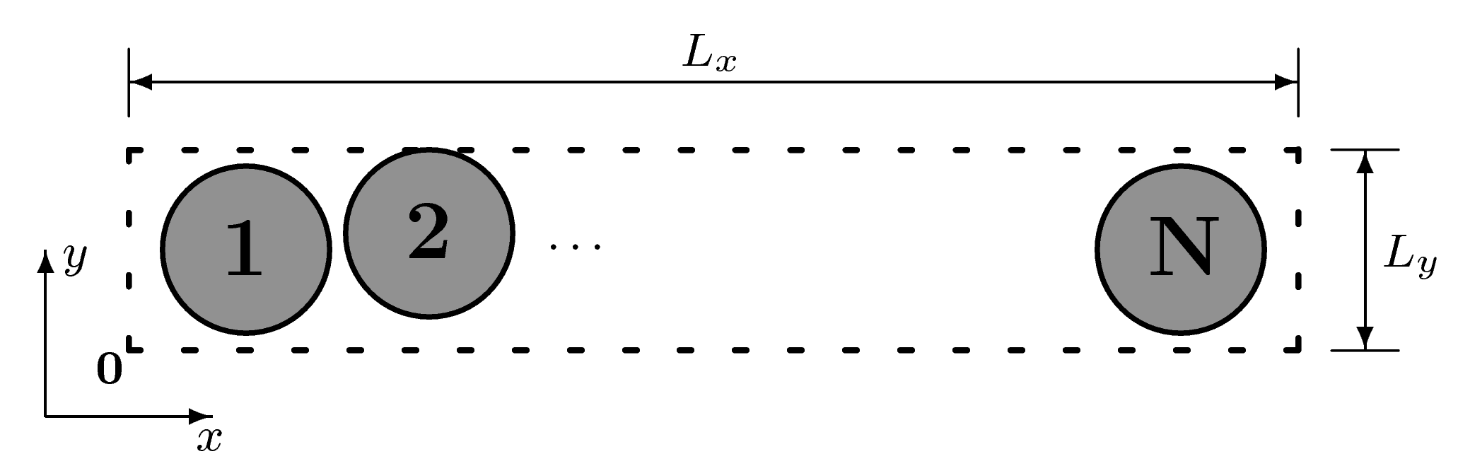
In nonequilibrium thermodynamics the kinetic-theory basis of the heat transport model in quasi-one-dimensional (QOD) systems has been discussed recently [14]. The basic ingredient [15,16] is the Boltzmann entropy $S\left(t\right)$ which is defined, up to a constant, to be

$$S\left(t\right)=\int d\mathbf{r}s(\mathbf{r},t)=-\int d\mathbf{r}\int d\mathbf{v}f(\mathbf{r},\mathbf{v},t)lnf(\mathbf{r},\mathbf{v},t)$$

(3)

where $s(\mathbf{r},t)$ is the entropy density at position $\mathbf{r}$ at time t and we take Boltzmann’s constant to equal one. The Boltzmann entropy is just the kinetic contribution and the configurational contribution written in terms of correlation functions is often referred to as the Green entropy [17]. We assume that the system has reached a steady state so that the entropy, and all other thermodynamic properties, no longer depend on time. The distribution function $f(\mathbf{r},\mathbf{v},t)=n(\mathbf{r},t)P(\mathbf{r},\mathbf{v},t)$ obeys the Boltzmann equation, which without external forces takes the following form

$$\frac{\partial f}{\partial t}+\mathbf{v}·\frac{\partial f}{\partial \mathbf{r}}=J\left[f\right]$$

(4)

where $J\left[f\right]$ is the collision integral and $P(\mathbf{r},\mathbf{v},t)$ is the momentum probability density. The distribution function is normalized so that

$$\int d\mathbf{v}f(\mathbf{r},\mathbf{v},t)=n(\mathbf{r},t)$$

(5)

where $n(\mathbf{r},t)$ is the local number density of the system. The local entropy-balance equation is obtained by using the Boltzmann equation, Equation (4), to calculate the total time-derivative of the Boltzmann entropy, Equation (3). When the fluid is on average stationary, the result is expressed as

$$\frac{\partial s}{\partial t}+\nabla ·{\mathbf{j}}_s={\sigma }_{ent}$$

(6)

where ${\mathbf{j}}_s$ is the entropy flux and ${\sigma }_{ent}$ is the entropy production. The kinetic contribution to the entropy flux ${\mathbf{j}}_s$ is given by

$${\mathbf{j}}_s\left(\mathbf{r}\right)=-\int d\mathbf{v}\mathbf{v}flnf$$

(7)

The entropy-production per unit volume ${\sigma }_{ent}$ is given exactly by the first equality in Equation (8). However, the collision integral is too difficult to handle so we approximate it using the BGK approximation as $J\left[f\right]=\nu (f\left(\mathbf{v}\right)-f_{loc}\left(\mathbf{v}\right))$, thus we can estimate ${\sigma }_{ent}$ as

$${\sigma }_{ent}\left(\mathbf{r}\right)=-\int d\mathbf{v}J\left[f\right]lnf=\nu \left(\mathbf{r}\right)\int d\mathbf{v}\{f\left(\mathbf{v}\right)-f_{loc}\left(\mathbf{v}\right)\}lnf\left(\mathbf{v}\right)$$

(8)

where $\nu \left(\mathbf{r}\right)$ is the local relaxation frequency proportional to ${\nu }_{0}n\left(\mathbf{r}\right)\sqrt{T\left(\mathbf{r}\right)}$ (${\nu }_0$ is a constant that depends on dimensionality). According to the H-theorem [18] ${\sigma }_{ent}\left(\mathbf{r}\right)$ must be positive. All the local quantities associated with the entropy balance equation have been defined through the Boltzmann equation and their definitions are exact within its validity and are not restricted to the linear regime. In the Chapman–Enskog expansion solution to first order in the gradient (that is Navier–Stokes order [19]) the distribution function is given by $f=f_{loc}(1+\Phi )$, where $f_{loc}$ is the local-equilibrium distribution function, which is a Gaussian at the local temperature and number density.

3. The Model System

To specify the thermal contact between system and reservoir, it is necessary to move from a macroscopic picture to a microscopic one, describing the collision process that allows energy to flow at the system-reservoir boundary. We can separate simplified reservoir models into two classes; stochastic and deterministic. A typical stochastic model uses Gaussian reservoirs to provide a source of thermalized particles from a Gaussian distribution at a set temperature. These reservoirs cannot sense the temperature as they are simply sources of thermalized particles.

The QOD system introduced recently [20] can be modified to interact with an idealized mechanical heat reservoir in a deterministic and reversible way [21], to study both heat conduction in low dimensional systems and the Lyapunov mode structure. The deterministic reservoir allows the calculation of the usual dynamical systems properties as well as the thermodynamic properties. Similar systems have been used recently to study heat flow [22,23], Eckmann and Young [24] have developed Hamiltonian and stochastic models for heat transport in low dimensional systems. The Hamiltonian models consist of energy storage devices which couple to each other through the motion of tracer particles that carry the energy. Although these models principally store energy as rotational kinetic energy, they are similar in many ways to the QOD system considered here which store energy locally in the y degree of freedom. If we envisage taking the QOD system, expanding odd numbered disks to twice their diameter and shrinking the even numbered ones to points, we obtain a scatterer-tracer system but with tracers always confined between the same two scatterers. The chaotic scattering of hard disks in two-dimensions gives a mechanism to transfer energy between particles with different momentum components, and hence may be more realistic than one-dimensional models particularly for fluid systems.

3.1. System Dynamics

The QOD system contains N hard disks of diameter $\sigma =1$ and mass $m=1$ in a narrow channel $L_x\times L_y$ where the system width is less than twice the particle diameter $L_y<2\sigma$ so that the disks remain ordered (see Figure 1). As the position of the $i^{th}$ particle is restricted to lie between particles $i-1$ and $i+1$ any property of particle i can be associated with the same local density at the average position $〈x_i〉$ of particle i. For example, the local number density $n(\mathbf{r},t)$ is the inverse of the average volume occupied by the particle ${\rho }_i=1/V_i$ where $V_i=L_y\left(〈x_{i+1}-x_{i-1}〉\right)/2$.

The equations of motion connecting the QOD system to the two reservoirs at $x=0$ and $L_x$ define the thermal contact. When a particle collides with a reservoir wall the usual collision rule in the x direction is replaced by

$$p_x^{\prime }=ϵp_I-(1-ϵ)p_x$$

(9)

where $p_I=\pm \sqrt{2T_I}$ is the fixed value of the reservoir momentum for the $I^{th}$ reservoir (either $p_L$ for the left-hand side or $p_R$ for the right-hand side) for a given boundary temperature of $T_I$. Note that the reservoir momentum is always directed from the reservoir into the system; so here $p_L>0$ and $p_R<0$. We use a system width of $L_y=1.15\sigma$, allowing $L_x$ to vary with the number of particles N to give the desired density $\rho =N{\sigma }^2/\left(L_x{L}_y\right)$. The temperature profile is determined from the average components of the kinetic temperature of each particle [the average of Equation (2)].

Figure 1. Schematic presentation of an N hard-disk quasi-one-dimensional (QOD) system. The height $L_y$ is sufficiently small that the disks cannot pass one another. We choose the coordinate origin to be located at the bottom left corner of the system, and system boundaries are denoted by dashed lines. The boundaries at $x=0$ and $L_x$ are hard walls and those at $y=0,L_y$ periodic (that is, a (H,P) quasi-one-dimensional system).

Figure 1. Schematic presentation of an N hard-disk quasi-one-dimensional (QOD) system. The height $L_y$ is sufficiently small that the disks cannot pass one another. We choose the coordinate origin to be located at the bottom left corner of the system, and system boundaries are denoted by dashed lines. The boundaries at $x=0$ and $L_x$ are hard walls and those at $y=0,L_y$ periodic (that is, a (H,P) quasi-one-dimensional system).

The parameter ϵ represents the strength of the coupling between the reservoir and the system. If $ϵ=0$ there is no interaction with the reservoir, while if $ϵ=1$ the incoming momentum is completely replaced by the reservoir momentum. Here we use an intermediate value of $ϵ=0.5$, which provides an effective mix of the incoming momentum with the reservoir momentum. The physical interpretation of Equation (9) is straightforward; when a collision occurs with a reservoir the reflected particle has the x component of its momentum changed to a linear combination of the reservoir momentum and its momentum before collision. This results in a strong peak in the reflected momentum near the value of the reservoir momentum which is broadened due to the randomness of the incoming particle momentum, shown in Figure 2. This produces a probability density $P(\mathbf{r},\mathbf{v})$ which is quite different from Gaussian at the local temperature and density. Through interactions with other particles this reflected momentum distribution returns to a more Gaussian-like distribution after four or five particles, regardless of N.

Figure 2. The probability density divided by the local Gaussian probability density for the velocity of particles 1, $N/2$ and N respectively in an N hard-disk quasi-one-dimensional (QOD) system with reservoirs at the same temperature. Particles 1 and N are nearest the two reservoirs so their probability densities in $v_x$ are mirrored, while particle $N/2$ is in the middle of the QOD system. The horizontal axis is $v_x$ and the vertical axis is $v_y$ with the colour scale for the probability on the right-hand side. The probability density for particle 1 shows a strong injection peak around the reservoir velocity which is positive. The probability density for particle $N/2$ is essentially equal one everywhere except for $v_x^2+v_y^2>6^2$ where the numerical probability density is zero (thus colored red).

Figure 2. The probability density divided by the local Gaussian probability density for the velocity of particles 1, $N/2$ and N respectively in an N hard-disk quasi-one-dimensional (QOD) system with reservoirs at the same temperature. Particles 1 and N are nearest the two reservoirs so their probability densities in $v_x$ are mirrored, while particle $N/2$ is in the middle of the QOD system. The horizontal axis is $v_x$ and the vertical axis is $v_y$ with the colour scale for the probability on the right-hand side. The probability density for particle 1 shows a strong injection peak around the reservoir velocity which is positive. The probability density for particle $N/2$ is essentially equal one everywhere except for $v_x^2+v_y^2>6^2$ where the numerical probability density is zero (thus colored red).

3.2. Energy Balance

In a numerical simulation we can calculate the energy flux between system and reservoir by direct calculation or we can calculate it indirectly through the probability density of incident momentum and the collision frequency. Once obtained, the probability density of incident momentum $p_x$ will give all of the fluxes to and from the reservoirs per collision. The number of collisions per unit time $n_L$ with momentum $-p_x$ on the left-hand wall is given by the product of, the length of the collision cylinder $|p_x|\delta t$ for particles which collide within time $\delta t$, and the probability density that a particle has momentum $-p_x$ is given by $P(-p_x)$. Thus the number of collisions for particles with momentum $p_x$ is $n_L\delta t=\left|p_x\right|exp(-\frac{1}{2}\beta p_x^2)\delta t$ and the normalized incoming wall collision probability density is $P\left(p_x\right)=\beta \left|p_x\right|exp(-\frac{1}{2}\beta p_x^2)$. To calculate the energy balance at the left-hand reservoir we use the wall collision distribution and calculate the average energy transfer $〈{p^{\prime }}_x^2-p_x^2〉$. Using the collision rule from Equation (9) and taking the wall momentum as $p_L=\sqrt{2T_L}$, we look for the value of β for which there is on average no energy transfer in a collision. Therefore we require that

$$ϵp_L^2+2(ϵ-1)〈p_x〉p_L+(ϵ-2)〈p_x^2〉=0$$

(10)

The probability density for the incoming momenta gives $〈p_x〉=-\sqrt{\pi /2\beta }$ and $〈p_x^2〉=2/\beta$, where the incoming collisional temperature $T=1/\beta$. We then obtain a quadratic equation for $\sqrt{T/T_L}$,

$$\frac{T}{T_L}-\sqrt{\pi }\frac{(ϵ-1)}{(ϵ-2)}\sqrt{\frac{T}{T_L}}+\frac{ϵ}{(ϵ-2)}=0$$

(11)

Solving this equation gives

$$T=\frac{\sqrt{\pi }}{2}\frac{(ϵ-1)}{(ϵ-2)}\left\{1\pm \sqrt{1-\frac{4ϵ(ϵ-2)}{\pi {(ϵ-1)}^2}}\right\}{T}_L$$

(12)

Note that as $ϵ-2$ is always negative when $1>ϵ>0$, the term inside the square root is always positive. Here we have chosen a temperature to associate with the incoming momentum distribution and found the value which produces an energy balance at the boundary. In this analysis the temperature T only depends on the value of ϵ, not on the system size N or the density ρ. As a concrete example, we consider a QOD system of 640 hard disks at density $\rho =0.8$ connected to reservoirs with equal temperatures $T_L=T_R=2$, which gives a fitted incoming momentum probability density $P\left(p_x\right)=\alpha p_{x}exp(-\frac{1}{2}\beta p_x^2)$ where $\alpha =0.547$ and $\beta =0.537$, implying $T=1.862$. This is not a good fit to the data and for the distribution to be properly normalised we require $\alpha =\beta$. For $ϵ=1/2$, there is only one physical solution to Equation (12), $T=1.78152$, independent of both N and ρ. Whether this temperature should be associated with the particle closest to the boundary or some other bulk measure of the temperature is not immediately clear. In Table 1 we observe that the x and y temperatures of particle 1 converge quickly with increasing N, but to different values, and $T_x$ is greater than the boundary temperature of 2.

Table 1. The temperature of the left-hand boundary particle - particle 1 - for QOD systems as a function of system size with fixed reservoir temperatures of $T_L=T_R=2$. The first two columns are for a density $\rho =0.03$ while the last two columns are for a density $\rho =0.8$. This data is also contained in Figure 3.

N	${\mathit{T}}_{\mathit{x}}\mathbf{\left(}\mathbf{1}\mathbf{\right)}$	${\mathit{T}}_{\mathit{y}}\mathbf{\left(}\mathbf{1}\mathbf{\right)}$	${\mathit{T}}_{\mathit{x}}\mathbf{\left(}\mathbf{1}\mathbf{\right)}$	${\mathit{T}}_{\mathit{y}}\mathbf{\left(}\mathbf{1}\mathbf{\right)}$
80	$2.1270$	$1.8241$	$2.0836$	$1.7796$
160	$2.1205$	$1.8271$	$2.0785$	$1.7852$
320	$2.1179$	$1.8313$	$2.0755$	$1.7837$
640	$2.1157$	$1.8320$	$2.0750$	$1.7832$
1280	$2.1147$	$1.8333$	−	−

Table 1. The temperature of the left-hand boundary particle - particle 1 - for QOD systems as a function of system size with fixed reservoir temperatures of $T_L=T_R=2$. The first two columns are for a density $\rho =0.03$ while the last two columns are for a density $\rho =0.8$. This data is also contained in Figure 3.

N	${\mathit{T}}_{\mathit{x}}\mathbf{\left(}\mathbf{1}\mathbf{\right)}$	${\mathit{T}}_{\mathit{y}}\mathbf{\left(}\mathbf{1}\mathbf{\right)}$	${\mathit{T}}_{\mathit{x}}\mathbf{\left(}\mathbf{1}\mathbf{\right)}$	${\mathit{T}}_{\mathit{y}}\mathbf{\left(}\mathbf{1}\mathbf{\right)}$
80	$2.1270$	$1.8241$	$2.0836$	$1.7796$
160	$2.1205$	$1.8271$	$2.0785$	$1.7852$
320	$2.1179$	$1.8313$	$2.0755$	$1.7837$
640	$2.1157$	$1.8320$	$2.0750$	$1.7832$
1280	$2.1147$	$1.8333$	−	−

Figure 3. The temperature profiles $T_x$ (red symbols) and $T_y$ (blue symbols) as a function of $X=(i-0.5)/N$ where i is the particle index for QOD systems of $80,160,320$ and 640 hard-disks with $T_L=T_R=2$. Plot (a) is the result for $\rho =0.03$ and (b) is the result for $\rho =0.8$. These profiles are strongly dependent on system size with the bulk temperature smaller with increasing N and there are local differences between $T_x$ and $T_y$. The results are remarkably insensitive to density with only very slightly smaller values at the higher density.

Figure 3. The temperature profiles $T_x$ (red symbols) and $T_y$ (blue symbols) as a function of $X=(i-0.5)/N$ where i is the particle index for QOD systems of $80,160,320$ and 640 hard-disks with $T_L=T_R=2$. Plot (a) is the result for $\rho =0.03$ and (b) is the result for $\rho =0.8$. These profiles are strongly dependent on system size with the bulk temperature smaller with increasing N and there are local differences between $T_x$ and $T_y$. The results are remarkably insensitive to density with only very slightly smaller values at the higher density.

The best predicted temperature T is very close to $T_y$ at $\rho =0.8$, but different from the low density result. Numerically, we find that a two parameter form for the probability density gives a much better fit (see Figure 4),

$$P_L\left(p_x\right)=(\alpha p_x+\gamma p_x^2)exp(-\beta p_x^2/2)$$

(13)

and the temperature is more consistent with the temperature at the centre of the system. When $\gamma =0$, $\alpha =\beta$ and this reduces to the simpler distribution. This distribution can also be used to calculate the energy balance or flux across the boundary by considering the average per collision $〈{p^{\prime }}_x^2-p_x^2〉$ and multiplying this by the collision frequency (for collisions with reservoir I). The parameters for the fits to the incoming momentum probabilities, shown in Table 2, are remarkably insensitive to system size N.

Figure 4. The probability density of incoming momentum (dots) and its functional fit (line) for both the left and right hand reservoirs for a QOD system of 80 hard-disks at a density $\rho =0.8$ with $ϵ=0.5$ and reservoir temperatures $T=2$. Note that all incoming momenta for the left hand reservoir must be negative so $P_L\left(p_x\right)=0$ for $p_x>0$. Similarly, $P_R\left(p_x\right)=0$ for $p_x<0$. The functional form [Equation (13)] is an excellent fit to the data for both boundary distributions.

Figure 4. The probability density of incoming momentum (dots) and its functional fit (line) for both the left and right hand reservoirs for a QOD system of 80 hard-disks at a density $\rho =0.8$ with $ϵ=0.5$ and reservoir temperatures $T=2$. Note that all incoming momenta for the left hand reservoir must be negative so $P_L\left(p_x\right)=0$ for $p_x>0$. Similarly, $P_R\left(p_x\right)=0$ for $p_x<0$. The functional form [Equation (13)] is an excellent fit to the data for both boundary distributions.

Table 2. Parameters for the incoming momentum distributions at the left-hand side of QOD systems as a function of system size at density $\rho =0.8$ with reservoir temperatures of$T_L=T_R=2$.

N	α	β	γ	T
80	$-0.45624$	$0.62897$	$0.1098$	$1.5899$
160	$-0.45850$	$0.62913$	$0.1084$	$1.5895$
320	$-0.45904$	$0.62954$	$0.1082$	$1.5885$
640	$-0.45946$	$0.63001$	$0.1084$	$1.5895$

Table 2. Parameters for the incoming momentum distributions at the left-hand side of QOD systems as a function of system size at density $\rho =0.8$ with reservoir temperatures of$T_L=T_R=2$.

N	α	β	γ	T
80	$-0.45624$	$0.62897$	$0.1098$	$1.5899$
160	$-0.45850$	$0.62913$	$0.1084$	$1.5895$
320	$-0.45904$	$0.62954$	$0.1082$	$1.5885$
640	$-0.45946$	$0.63001$	$0.1084$	$1.5895$

To produce a nonequilibrium steady state it is sufficient to have reservoirs of different temperatures on each side of the QOD system. The energy entering the system from a boundary with reservoir momentum $p_I$ during a collision with a particle of incoming momentum $p_x$ is given by

$$\Delta e_I=\frac{1}{2}({p^{\prime }}_x^2-p_x^2)=\frac{ϵ}{2}[ϵp_I^2+2(ϵ-1)p_I{p}_x+(ϵ-2)p_x^2]$$

(14)

The time average of this quantity gives the flux of energy into the system so for a total system energy balance $\Delta e_L$ must be equal in magnitude but opposite in sign to $\Delta e_R$. The energy flux is controlled by both the reservoir momentum $p_I$, the value of ϵ, and the probability distribution for the incoming momentum, and goes to zero as $ϵ\to 0$.

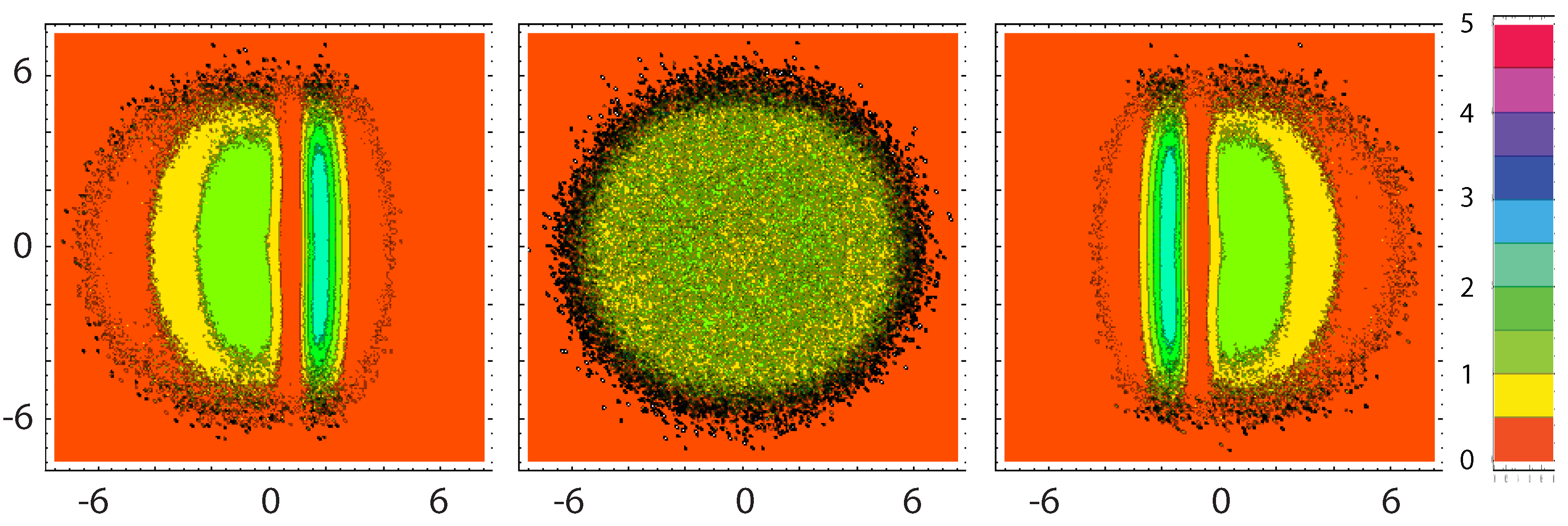
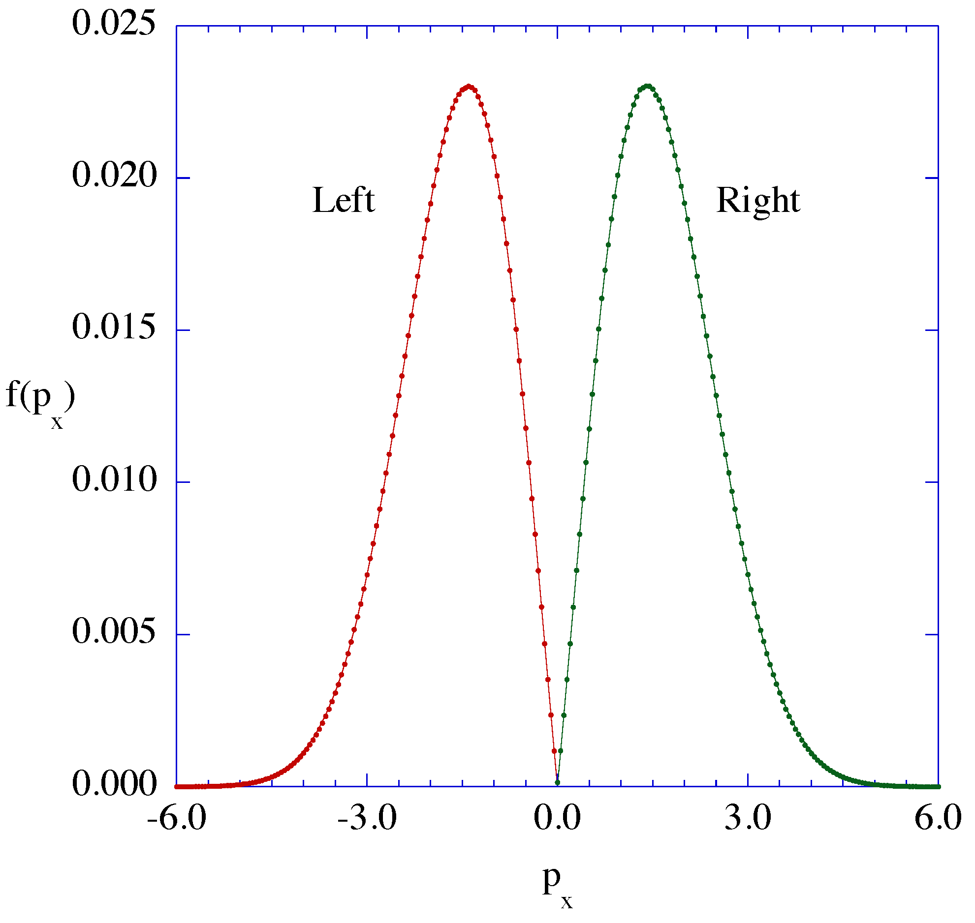
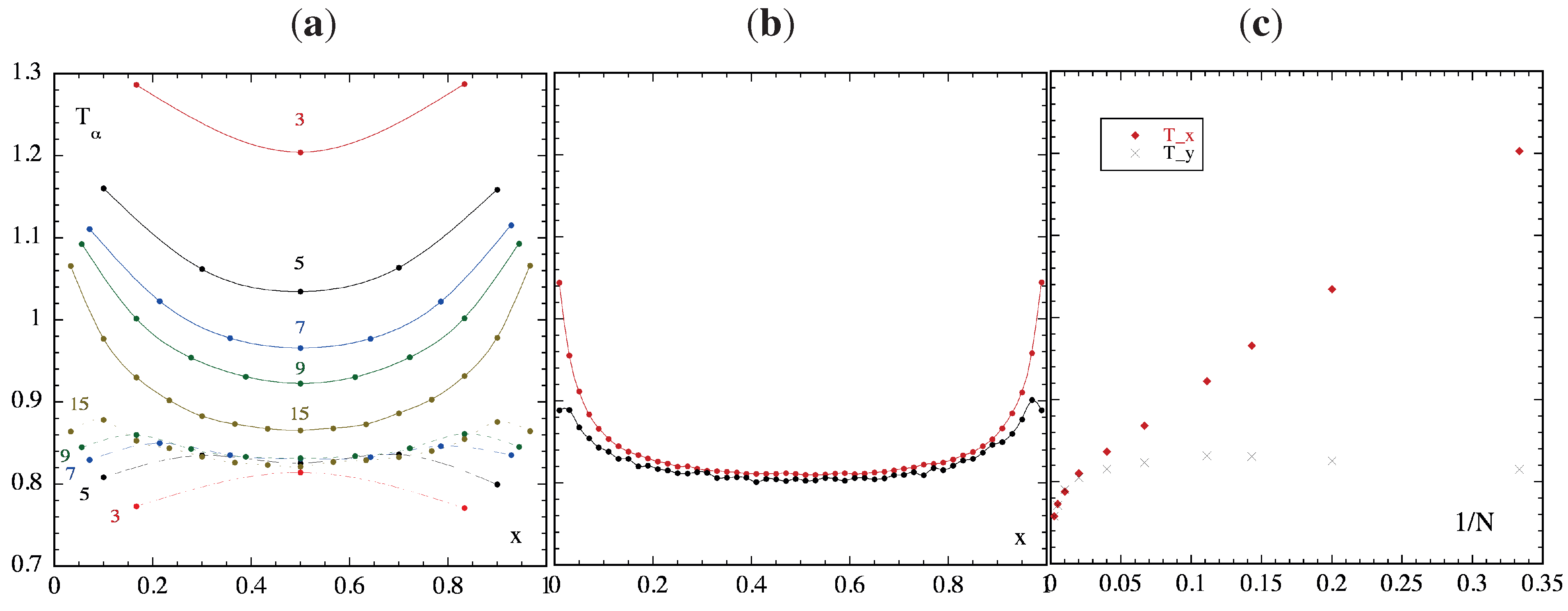
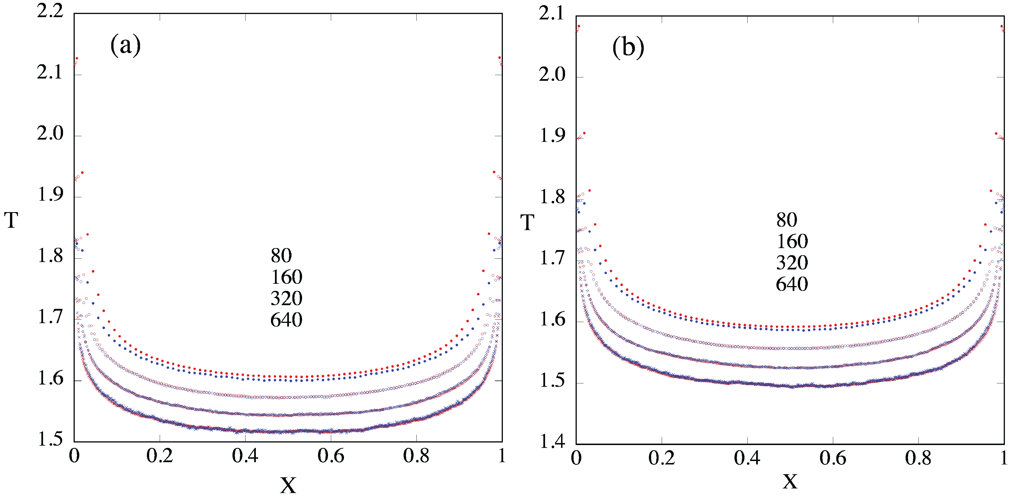
3.3. Temperature Profiles

The generic picture used to construct the canonical ensemble is a system in contact with a heat reservoir; a system in contact with two reservoirs at the same temperature is both canonical and in equilibrium with both reservoirs. In a mechanical dynamical system we expect that an arbitrary initial condition after some transient (a large number of collisions) will come to an equilibrium state, independent of the initial configuration, and remain there indefinitely. After this transient, there is no average energy transfer between system and reservoir. In the equilibrium state the components of the local kinetic temperature, $T_x$ and $T_y$, would be expected to become equal, $T_x=T_y$. For the QOD system the temperature profiles can be presented as either functions of the average position of the particle, or as a function of particle number (as the order is fixed), but to be able to compare systems of different size we use a simple scaling function $X=(i-0.5)/N$ where i is the particle number. Figure 5 shows both x and y components of the temperature profile for QOD systems of 3 to 50 disks connected to two reservoirs with the same temperatures $T_L=T_R=1$ as a function of $x=(i-0.5)/N$. For these small systems the temperature profiles show very strong number dependence and there is no evidence of equilibration between x and y temperatures before the system size nears 50, but even here $〈T_x〉>〈T_y〉$ everywhere in the system. The drop in $〈T_y〉$ for the two particles in contact with the reservoirs is a consistent feature in all profiles. Further, the temperature in the centre of the system is significantly lower than the temperature of the reservoirs and this varies with system size. The direct numerical calculation of the $p_x$ and $p_y$-distributions gives good fits to Gaussians with temperatures equal to local kinetic x and y temperatures, away from the boundaries, thus the second moment calculated from the distribution is consistent with that calculated directly.

A systematic study of the temperature profile for larger systems shows that the same behaviour persists but becomes smaller with increasing N (see Figure 3). There is a strong dependence on system size as the bulk T is lowered with increasing N with no indication that the profiles will converge to some universal $N\to \infty$ limit. The profiles seem almost completely independent of the density, as can be seen by comparing the two graphs in Figure 3. Although the temperature difference between the boundary and particle 1 is not given by the analysis above, we can construct an argument for the systematically lower temperatures in the centre of the QOD systems as N increases. As the difference in temperature between the boundary and $T_y\left(1\right)$ is independent of N and decreases monotonically with particle number with the same slope regardless of N, a larger system size will lead to a larger decrease and thus a lower centre temperature.

Figure 5. (a) The temperature profiles $T_x$ (top) and $T_y$ (bottom) as a function of X for QOD systems of $3,5,7,9$ and 15 hard-disks at $\rho =0.8$ as a function of $X=(i-0.5)/N$. These profiles are strongly dependent on system size and there are significant differences between $T_x$ and $T_y$ for the smaller systems. (b) The temperature profiles for a QOD system of 50 hard-disks showing that despite good equilibration of $T_x$ and $T_y$ locally, there remains a systematic difference between the two temperatures with $T_x>T_y$. (c) The temperature of the middle particle(s) in the QOD systems of different size plotted against $1/N$. Whilst initially appearing to converge, for systems of more than 100 disks the change in temperature with system size increases. Notice that the temperature near the centre is more than $20\%$ smaller than the nominal reservoir temperature $T=1$. All graphs have the same vertical scale.

Figure 5. (a) The temperature profiles $T_x$ (top) and $T_y$ (bottom) as a function of X for QOD systems of $3,5,7,9$ and 15 hard-disks at $\rho =0.8$ as a function of $X=(i-0.5)/N$. These profiles are strongly dependent on system size and there are significant differences between $T_x$ and $T_y$ for the smaller systems. (b) The temperature profiles for a QOD system of 50 hard-disks showing that despite good equilibration of $T_x$ and $T_y$ locally, there remains a systematic difference between the two temperatures with $T_x>T_y$. (c) The temperature of the middle particle(s) in the QOD systems of different size plotted against $1/N$. Whilst initially appearing to converge, for systems of more than 100 disks the change in temperature with system size increases. Notice that the temperature near the centre is more than $20\%$ smaller than the nominal reservoir temperature $T=1$. All graphs have the same vertical scale.

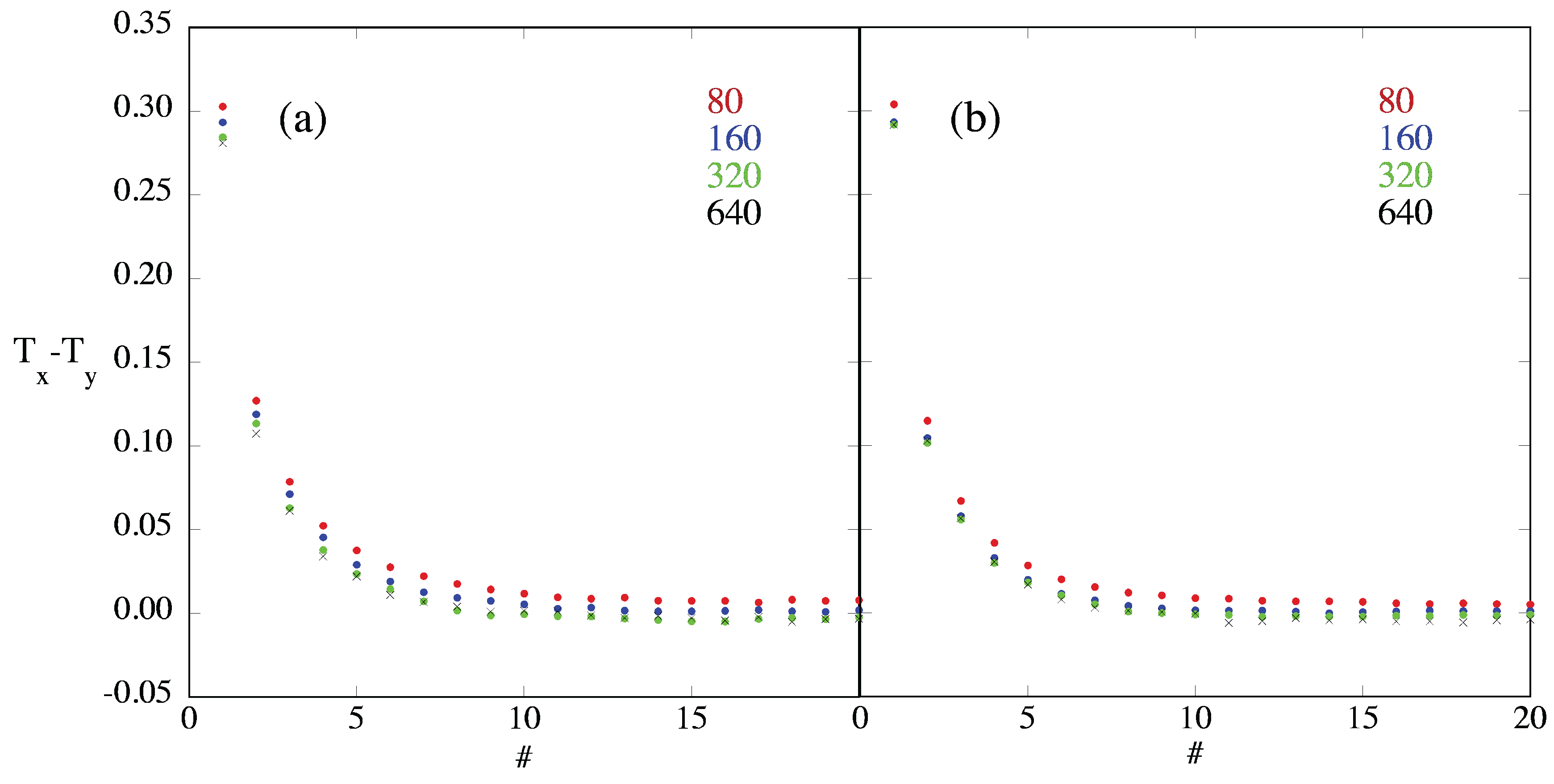
3.4. Temperature Differences and Equilibration

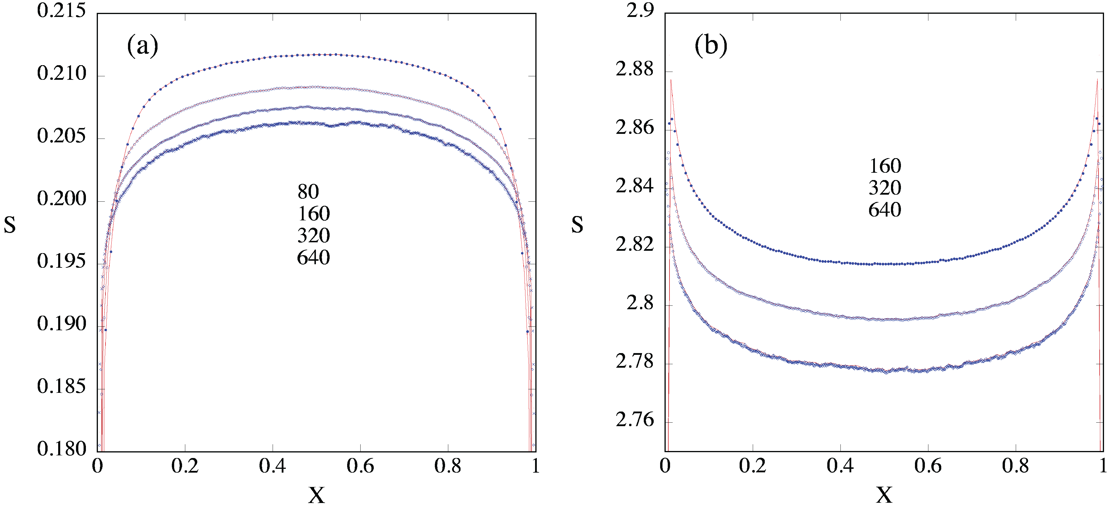
The temperature differences $T_x-T_y$ as a function of particle number are shown in Figure 6 for both low density and high density systems and we see in both cases that the effects are mostly visible in the first ten particles regardless of the system size and the density. We will refer to this behaviour as an order one effect as it is independent of system size N and always involves the same number of particles near a boundary. For 80 and 160 particles $T_x>T_y$ so nowhere in the system is the temperature fully equilibrated. At the larger system sizes of 320 and 640 particles the results for $T_x-T_y$ look like noise with a mean of zero, so the temperature has equilibrated. Thus the temperature equilibration in the bulk of the system is an order N effect, requiring somewhere between 160 and 320 particles, but near both boundaries there is a region of approximately 10 particles that never equilibrate.

Figure 6. The temperature difference $T_x-T_y$ profiles as a function of the particle index for QOD systems of $80,160,320$ and 640 hard-disks with $T_L=T_R=2$. The vertical scale on both graphs is the same. (a) Results for $\rho =0.03$ and (b) Results for $\rho =0.8$. These profiles are remarkably independent of system size N and density ρ.

Figure 6. The temperature difference $T_x-T_y$ profiles as a function of the particle index for QOD systems of $80,160,320$ and 640 hard-disks with $T_L=T_R=2$. The vertical scale on both graphs is the same. (a) Results for $\rho =0.03$ and (b) Results for $\rho =0.8$. These profiles are remarkably independent of system size N and density ρ.

4. Entropy

We consider a steady system with reservoirs of equal temperature at each end. As can be seen from Figure 3 and Figure 5, even in the absence of an external temperature gradient both the x and y temperatures vary with position and are generally not equal. The Chapman–Enskog expansion solution, to first order in the gradient of the distribution function, is given by $f=f_{loc}(1+\Phi )$ where $f_{loc}$ is the local-equilibrium distribution function, ${\beta }_x=1/T_x$ and ${\beta }_y=1/T_y$ depend upon x and are allowed to differ locally. Then $f_{loc}$ can be written as

$$f_{loc}(x,\mathbf{v})=\frac{mn\left(x\right)}{2\pi }{\left({\beta }_x{\beta }_y\right)}^{1/2}exp\left[-\frac{m}{2}\left({\beta }_x{v}_x^2+{\beta }_y{v}_y^2\right)\right]$$

(15)

The right-hand side depends on x through $n\left(x\right)$, ${\beta }_x$ and ${\beta }_y$. This is an extension of the local equilibrium concept to a system which can have differing temperatures in the x and y directions as is commonly found for nonequilibrium steady states [25]. The entropy density is obtained at the level of the local-equilibrium approximation as

$$s_{loc}\left(x\right)\simeq -\int d\mathbf{v}{f}_{loc}ln{f}_{loc}=n\left(x\right)\left\{1-ln\left[\left(\frac{mn\left(x\right)}{2\pi }\right){\left({\beta }_x{\beta }_y\right)}^{1/2}\right]\right\}$$

(16)

This entropy density obtained is reminiscent of the equilibrium Sackur–Tetrode equation, except here the hydrodynamic fields are local.

In the computer simulation of the QOD system a histogram of the velocity distribution for each particle is collected on a fixed grid size ζ. For a velocity distribution in two variables $P(v_x,v_y)$ the distribution at $v_x=v_i$ and $v_y=v_j$ is $f(i,j)=nP(v_x,v_y)$. The discrete distribution for each histogram cell $f_{i,j}$ is the integral of the probability distribution $f(i,j)$ over the cell so $f_{ij}=\int f(i,j)d\mathbf{v}\simeq f(i,j){\zeta }^2$ so that $f(i,j)=f_{ij}/{\zeta }^2$. The entropy can then be calculated for each particle as follows

$$s=-\int d\mathbf{v}flnf\simeq -\sum _{i,j}{\zeta }^{2}f(i,j)lnf(i,j)=-\sum _{i,j}{f}_{i,j}ln{f}_{i,j}+2nln\zeta$$

(17)

The convergence of the entropy density $s\left(x\right)$ and the local equilibrium entropy density $s_{loc}\left(x\right)$ is quite different. The entropy density requires the convergence of the numerical velocity distribution itself while the local equilibrium entropy density only requires the convergence of the field variables $n\left(x\right)$, ${\beta }_x\left(x\right)$ and ${\beta }_y\left(x\right)$. In Figure 7 we see that $s_{loc}$ is an upper bound for s and the two entropies are in good agreement with each other. The number dependence of the entropy is similar to the the number dependence of the temperature as S becomes smaller with increasing N.

Figure 7. The entropy profiles $s\left(x\right)$ (blue symbols) and $s_{loc}\left(x\right)$ (red line) as a function of $X=(i-0.5)/N$ where i is the particle index for QOD systems of $80,160,320$ and 640 hard-disks with $T_L=T_R=2$. (a) are the results for $\rho =0.03$ and (b) are the results for $\rho =0.8$. These profiles are strongly dependent on system size. They change with system size but the agreement between $s_{loc}\left(x\right)$ and $s\left(x\right)$ is impressive in all cases. Note that $s_{loc}\left(x\right)>s\left(x\right)$ for all values of x. The largest difference between $s\left(x\right)$ and $s_{loc}\left(x\right)$ is at the boundaries where the momentum distributions deviate most greatly from Gaussian.

Figure 7. The entropy profiles $s\left(x\right)$ (blue symbols) and $s_{loc}\left(x\right)$ (red line) as a function of $X=(i-0.5)/N$ where i is the particle index for QOD systems of $80,160,320$ and 640 hard-disks with $T_L=T_R=2$. (a) are the results for $\rho =0.03$ and (b) are the results for $\rho =0.8$. These profiles are strongly dependent on system size. They change with system size but the agreement between $s_{loc}\left(x\right)$ and $s\left(x\right)$ is impressive in all cases. Note that $s_{loc}\left(x\right)>s\left(x\right)$ for all values of x. The largest difference between $s\left(x\right)$ and $s_{loc}\left(x\right)$ is at the boundaries where the momentum distributions deviate most greatly from Gaussian.

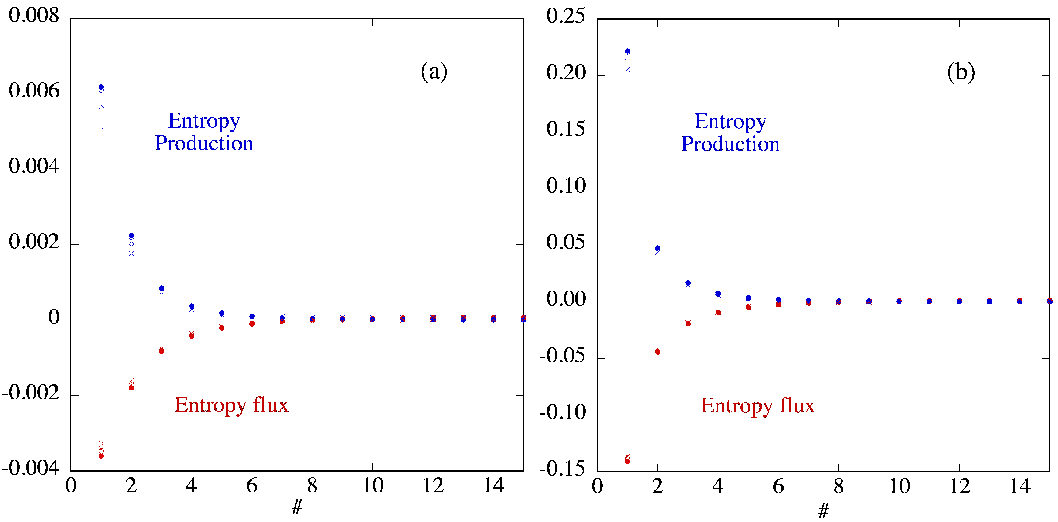
4.1. Entropy Production and Flux Near Reservoirs

It is surprising to find that despite the absence of entropy production and entropy flux in the bulk of the system, it is evident near the reservoirs. There is entropy production in this steady state system and an associated entropy flux directed into each reservoir. In Figure 8, the entropy production calculated from Equation (8) is concentrated on the particles closest to each of the reservoirs. The entropy properties come directly from the BGK approximation and the velocity probability density for each particle.

$${\sigma }_{ent}\left(x\right)=\nu \left(x\right)\int d\mathbf{v}\{f(x,\mathbf{v})-f_{loc}(x,\mathbf{v})\}lnf(x,\mathbf{v})$$

(18)

The two-dimensional velocity probability density for each particle $P\left(\mathbf{v}\right)$ is calculated numerically on a grid of typically $301\times 301$ with a resolution of $0.05$. The entropy, entropy flux and entropy production are all calculated numerically by integrating this probability density using Equations (3), (7), (8) with an error in the order of the square of the resolution, that is $0.0025$. The entropy flux and production are expected to be good representations at low density in the kinetic regime where $\rho <0.1$, but would neglect potential contributions at higher density. In the steady state $\frac{\partial s}{\partial t}=0$ so $\nabla ·{\mathbf{j}}_s={\sigma }_{ent}$. As both the entropy current and production are defined at each particle, we can associate these properties with the regions assigned to each particle and approximate the integral in Equation (18) as a sum.

$$j_m-j_{m+1}={\int }_{m+1}^m{\sigma }_{ent}\left(x\right)dx\sim -\Delta x_m{\nu }_m{a}_m$$

(19)

Here we can choose the particle number m freely and $\Delta x_m$ is related to the local density by ${\rho }_m=\frac{1}{\Delta x_m{L}_y}$. We have separated the entropy production into the product of two terms; the first is the local frequency parameter of the BGK approximation ${\nu }_m$, and the other is the integral of velocity probability density. Thus we can write ${\nu }_m$ in terms of known quantities calculated, using the BGK approximation only for $a_m$, and ask what value of ${\nu }_m$ is required to obtain consistent results. We have

$${\nu }_m=\frac{{\rho }_m{L}_y}{a_m}\left(j_{m+1}-j_m\right)$$

(20)

Figure 8. The entropy flux and entropy production plotted against particle number for an equilibrium QOD system of N hard-disks with $T_L=T_R=2$. System sizes used are $N=80$ (filled circles), 160 (open circles), 320 (open diamonds), 640 (crosses) and the results are remarkably insensitive to N. The entropy production is positive near the boundary and the entropy flux is directed into the boundary (reservoirs). Panel (a) is for and $\rho =0.03$, (b) is for $\rho =0.8$.

Figure 8. The entropy flux and entropy production plotted against particle number for an equilibrium QOD system of N hard-disks with $T_L=T_R=2$. System sizes used are $N=80$ (filled circles), 160 (open circles), 320 (open diamonds), 640 (crosses) and the results are remarkably insensitive to N. The entropy production is positive near the boundary and the entropy flux is directed into the boundary (reservoirs). Panel (a) is for and $\rho =0.03$, (b) is for $\rho =0.8$.

In Figure 8 we see that for a system in contact with two the equal reservoirs the entropy production is confined to a small number of particles nearest the wall and that the entropy production is largely independent of the system size (thus order one). The entropy production in a system with equal reservoirs is intensive, and only involves properties of the particles that are in contact with the reservoirs. The numerical convergence of these two quantities is quite different; the entropy production converges with the smoothness of the distribution increasing slowly and monotonically near the reservoirs and decreasing in the central part until a steady value is reached. Statistically, the probability density needs to be sampled sufficiently to obtain a reliable value over the whole two-dimensional space $(v_x,v_y)$ and the convergence of the local distribution depends on the convergence to the local fields $n\left(x\right)$, $T_x\left(x\right)$ and $T_y\left(x\right)$.

Using Equation (20) we calculate the BGK frequency that is required to give the simulation results that we observe in Figure 8. These results are plotted in Figure 9 and give a required frequency of about $0.02$ at the lower density of $0.03$, and a frequency of about $0.6$ at the higher density of $0.8$. The single particle collision frequency is independent of system size N and is about $2.5$ times larger than the BGK frequency at $\rho =0.03$. At the higher density $\rho =0.8$ the single particle collision frequency is almost 20 times larger than the BGK frequency. This suggests that the BGK frequencies are not connected with the frequencies of collision events in the simulation but rather relate to the longer time scale associated with the relaxation of the distribution. Comparing the two BGK frequencies we see that they are consistent with a linear dependence on density but do not give particular support to that proposition.

Figure 9. The recalculated values of the BGK relaxation frequency from the entropy production and entropy flux of QOD systems of 80 (red filled circles) and 160 disks (blue filled diamonds) at two different densities with reservoir temperatures of $T_L=T_R=2$. System sizes used are $N=80,160$ and the results are insensitive to N. Panel (a) is for $\rho =0.03$, panel (b) is for $\rho =0.8$.

Figure 9. The recalculated values of the BGK relaxation frequency from the entropy production and entropy flux of QOD systems of 80 (red filled circles) and 160 disks (blue filled diamonds) at two different densities with reservoir temperatures of $T_L=T_R=2$. System sizes used are $N=80,160$ and the results are insensitive to N. Panel (a) is for $\rho =0.03$, panel (b) is for $\rho =0.8$.

In Table 3 we give the number of collisions per particle for the different system sizes and densities we have considered. The numerical results obtained here need to be qualified in the sense that the process of heat conduction in this system and the relaxation to a steady state is generally very slow. Although we base our interpretation on long simulations, we cannot be certain that other slower processes remain undetected.

Table 3. Simulation lengths given as the number of collisions per particle as a function of system size at the two different densities with reservoir temperatures of $T_L=T_R=2$.

N	$\mathit{\rho }\mathbf{=}\mathbf{0.03}$	$\mathit{\rho }\mathbf{=}\mathbf{0.8}$
80	$1\times {10}^8$	$2\times {10}^8$
160	$1.5\times {10}^8$	$2\times {10}^8$
320	$0.75\times {10}^8$	$0.875\times {10}^8$
640	$0.25\times {10}^8$	$0.375\times {10}^8$

Table 3. Simulation lengths given as the number of collisions per particle as a function of system size at the two different densities with reservoir temperatures of $T_L=T_R=2$.

N	$\mathit{\rho }\mathbf{=}\mathbf{0.03}$	$\mathit{\rho }\mathbf{=}\mathbf{0.8}$
80	$1\times {10}^8$	$2\times {10}^8$
160	$1.5\times {10}^8$	$2\times {10}^8$
320	$0.75\times {10}^8$	$0.875\times {10}^8$
640	$0.25\times {10}^8$	$0.375\times {10}^8$

5. Conclusions

We have investigated the consequences of a particular microscopic coupling model between a system of hard disks and a reservoir, which has the advantage of being relatively simple and deterministic. The modification to the collision rule at the system-reservoir boundary allows the system to come to a steady state where on average no energy flows between system and reservoir. We construct a qualitative argument for the energy balance that implies a lower temperature than the boundary temperature inside the system which is observed numerically. In this work we have considered reservoirs with equal temperatures to probe the microscopic mechanisms, but it is possible to have reservoirs of different temperatures to produce nonequilibrium steady states. Although the collision rule is deterministic, it does not correspond to deterministic thermostats often used in nonequilibrium steady states [26,27].

In all cases at fixed N the system comes to a steady state but the temperature profiles depend on the system size. For systems of 3 to 50 disks the steady state temperature profiles differ for the x and y directions, but as the size gets larger, somewhere between 160 and 320, local thermal equilibration occurs and $T_x\simeq T_y$. While these system size effects get smaller with increasing N it is still clear that the temperature in the centre of the system has not converged to a limit at $N=640$. Indeed numerically there is no indication that such a limit exists. Evidence that the reservoir affects the temperature profile near the boundary in the same way regardless of system size, leading to the same temperature gradient, suggests that the centre temperature will be smaller for larger system. This is observed numerically, but again the argument is only qualitative. The major unresolved question is whether a large system limit exists for a QOD system with these reservoirs.

As well as systematic changes in the temperature there are also systematic changes in the local entropy that occur with system size. These lead to lower values of entropy in the centre of the system at both low and high densities. Although it can be shown that the entropy derived from the local equilibrium distribution is an upper bound on the local entropy calculated from the numerical distributions, there is remarkable agreement between the two entropies in all circumstances.

The deterministic coupling mechanism produces entropy in particles near the reservoir and that entropy is transported as an entropy flux density into the reservoir. The expected equilibrium configuration of a system between two reservoirs of the same temperature leads to a system that has a steady kinetic temperature which is lower than the temperatures of the reservoirs. By considering the probability distributions of the momentum of particles near the boundary, as well as the details of the reservoir dynamics, we provide a microscopic explanation of this effect.

Two effects that are order one (or independent of N) are the temperature difference near the boundary $T_x-T_y$, and the entropy production and flow near a boundary. The temperature difference is independent of both N and ρ. The entropy production and flux is independent of N but does depend on the density. There is no energy flux or momentum flux associated with this entropy flux. These local effects that occur near the boundaries reinforce the picture of a reservoir with a strong effect on the system locally but sometimes propagates throughout the system, as we see in the profiles of temperature and entropy density. Such reservoir-system interactions are important in a wide variety of situations and here the analysis is made possible because the interaction is specified mechanically.

References

1. Hatano, T.; Sasa, S. Steady-state thermodynamics of Langevin systems. Phys. Rev. Lett. 2001, 86, 3463. [Google Scholar] [CrossRef] [PubMed]
2. Morriss, G.P.; Rondoni, L. On a definition of temperature in equilibrium and nonequilibrium systems. Phys. Rev. E 1999, 59, 5. [Google Scholar] [CrossRef]
3. Baranyai, A. Numerical temperature measurement in far from equilibrium model systems. Phys. Rev. E 2000, 61, 3306. [Google Scholar] [CrossRef]
4. Baranyai, A. Temperature of nonequilibrium steady-state systems. Phys. Rev. E 2000, 62, 5989. [Google Scholar] [CrossRef]
5. Jou, D.; Casas-Vazquez, J.; Lebon, G. Extended Irreversible Thermodynamics; Springer: Berlin, Germany, 2001. [Google Scholar]
6. Ottinger, H.C. Beyond Equilibrium Thermodynamics; Wiley: New York, NY, USA, 2005. [Google Scholar]
7. Ritort, F. Resonant nonequilibrium temperatures. J. Phys. Chem. B 2005, 109, 6787. [Google Scholar] [CrossRef] [PubMed]
8. Garriga, A.; Ritort, F. Mode-dependent nonequilibrium temperature in aging systems. Phys. Rev. E 2005, 72, 031505. [Google Scholar] [CrossRef]
9. Shokef, Y.; Shulkind, G.; Levine, D. Isolated nonequilibrium systems in contact. Phys. Rev. E 2007, 76, 030101. [Google Scholar] [CrossRef]
10. Lepri, S.; Livi, R.; Politi, A. Thermal conduction in classical low-dimensional lattices. Phys. Rep. 2003, 377, 1. [Google Scholar] [CrossRef]
11. Evans, D.J.; Morriss, G.P. Statistical Mechanics of Nonequilibrium Liquids, 2nd ed.; Cambridge University Press: Cambridge, UK, 2008. [Google Scholar]
12. Morriss, G.P.; Chung, T.; Angstmann, C. Thermal contact. Entropy 2008, 10, 786. [Google Scholar] [CrossRef]
13. Lumpkin, M.E.; Saslow, W.M.; Visscher, W.M. One-dimensional Kapitza conductance: Comparison of the phonon mismatch theory with computer experiments. Phys. Rev. B 1978, 17, 4295. [Google Scholar] [CrossRef]
14. Kim, C.S.; Morriss, G.P. Local entropy in a quasi-one-dimensional heat transport. Phys. Rev. E 2009, 80, 061137. [Google Scholar] [CrossRef]
15. McLennan, J.A. Introduction to Non-equilibrium Statistical Mechanics; Prentice-Hall: Englewood Cliffs, NJ, USA, 1989. [Google Scholar]
16. Zwanzig, R. Nonequilibrium Statistical Mechanics; Oxford University Press: New York, NY, USA, 2001. [Google Scholar]
17. Born, M.; Green, H.S. A general Kinetic Theory of Liquids; Cambridge University Press: London, UK, 1949; pp. 14–17. [Google Scholar]
18. Cercignani, C. The Boltzmann Equation and Its Applications; Spinger-Verlag: New York, NY, USA, 1988. [Google Scholar]
19. Dorfman, J.R.; van Beijeren, H. The kinetic theory of gases. In Statistical Mechanics, Part B: Time-Dependent Processes; Berne, B., Ed.; Plenum: New York, NY, USA, 1977. [Google Scholar]
20. Taniguchi, T.; Morriss, G.P. Boundary effects in the stepwise structure of the Lyapunov spectra for quasi-one-dimensional systems. Phys. Rev. E 2003, 68, 026218. [Google Scholar] [CrossRef]
21. Taniguchi, T.; Morriss, G.P. Lyapunov modes for a nonequilibrium system with a heat flux. Comptes Rendus Physique 2007, 8, 625. [Google Scholar] [CrossRef]
22. Deutsch, J.M.; Narayan, O. One-dimensional heat conductivity exponent from a random collision model. Phys. Rev. E 2003, 68, 010201. [Google Scholar] [CrossRef]
23. Deutsch, J.M.; Narayan, O. Correlations and scaling in one-dimensional heat conduction. Phys. Rev. E 2003, 68, 041203. [Google Scholar] [CrossRef]
24. Eckmann, J.P.; Young, L.S. Temperature profiles in Hamiltonian heat conduction. Europhys. Lett. 2004, 68, 790. [Google Scholar] [CrossRef]
25. Evans, D.J.; Morriss, G.P. Statistical Mechanics of Nonequilibrium Liquids, 2nd ed.; Cambridge University Press: Cambridge, UK, 2008. [Google Scholar]
26. Bright, J.N.; Evans, D.J.; Searles, D.J. New observations regarding deterministic, time-reversible thermostats and Gauss’s principle of least constraint. J. Chem. Phys. 2005, 122, 194106. [Google Scholar] [CrossRef] [PubMed]
27. Evans, D.J.; Searles, D.J.; Williams, S.R. Musings on thermostats. J. Chem. Phys. 2010, 133, 104106. [Google Scholar] [CrossRef] [PubMed]