Article

An Artificial Bee Colony Algorithm for the Job Shop Scheduling Problem with Random Processing Times

1
School of Economics and Management, Nanchang University, Nanchang 330031, China
2
Department of Automation, Tsinghua University, Beijing 100084, China
*
Author to whom correspondence should be addressed.
Entropy 2011, 13(9), 1708-1729; https://doi.org/10.3390/e13091708
Submission received: 13 July 2011 / Revised: 9 September 2011 / Accepted: 9 September 2011 / Published: 19 September 2011

Abstract

:
Due to the influence of unpredictable random events, the processing time of each operation should be treated as random variables if we aim at a robust production schedule. However, compared with the extensive research on the deterministic model, the stochastic job shop scheduling problem (SJSSP) has not received sufficient attention. In this paper, we propose an artificial bee colony (ABC) algorithm for SJSSP with the objective of minimizing the maximum lateness (which is an index of service quality). First, we propose a performance estimate for preliminary screening of the candidate solutions. Then, the K-armed bandit model is utilized for reducing the computational burden in the exact evaluation (through Monte Carlo simulation) process. Finally, the computational results on different-scale test problems validate the effectiveness and efficiency of the proposed approach.

1. Introduction

The job shop scheduling problem (JSSP) has been known as an extremely stubborn combinatorial optimization problem since the 1950s. In terms of computational complexity, JSSP is NP -hard in the strong sense [1]. It models an important decision problem in contemporary manufacturing systems, so extensive research has been conducted on JSSP. Due to its high complexity, the recent research has focused on the meta-heuristic approaches, such as genetic algorithm (GA) [2], estimation of distribution algorithm (EDA) [3], tabu search (TS) [4], particle swarm optimization (PSO) [5], ant colony optimization (ACO) [6], artificial bee colony (ABC) algorithm [7].
However, most existing research is based on the standard JSSP model, which means it is impossible to directly apply these algorithms in real-world scheduling scenarios. Especially, we emphasize the following two points.
(1)
Most research on JSSP has focused on the makespan criterion (i.e., minimizing the maximum completion time). However, in the make-to-order (MTO) manufacturing environment, due date related performances are apparently more relevant for decision makers, because the in-time delivery of goods is vital for maintaining a high service reputation. Therefore, the research that aims at minimizing lateness/tardiness in JSSP deserves more attention.
(2)
Most existing algorithms are designed for the deterministic JSSP, in which all the data (e.g., the processing times) are assumed to be fixed and precisely known in advance. In real-world manufacturing, however, the processing of operations is constantly affected by uncertain factors. Machine breakdowns, worker absenteeism, order changes, etc. can all lead to variations in the operation times. In this case, solving the deterministic JSSP will not result in a robust production schedule. Therefore, it is rewarding to focus more research effort on the stochastic JSSP.
In an attempt to overcome the drawbacks, in this paper we study the stochastic job shop scheduling problem (SJSSP) with the objective of minimizing maximum lateness ( L max ) in the sense of expectation. Compared with the standard JSSP, the studied SJSSP moves a step closer to the practical scheduling features. The main contribution of this paper is an efficient optimization approach based on artificial bee colony for solving SJSSP. The algorithm first uses a quick-and-dirty performance estimate to roughly evaluate the candidate solutions. Then, the selected promising solutions undergo a more accurate evaluation through simulation. In this process, a new computing budget allocation policy is adopted in order to promote the computational efficiency.
The rest of the paper is organized as follows. Section 2 briefly reviews the recent publications on stochastic job shop scheduling and artificial bee colony algorithms. Section 3 provides the formulation of SJSSP and an introduction to the standard ABC principles. Section 4 introduces an estimate for the objective function (maximum lateness). Section 5 describes the design of ABC for SJSSP in detail. Section 6 gives the computational results. Finally, some conclusions are made in Section 7.

2. Literature Review

2.1. The Stochastic Job Shop Scheduling Problem

Due to the inevitable uncertainties in manufacturing systems, SJSSP is more realistic than its deterministic counterpart. In SJSSP, the number of jobs is usually known in advance, while the processing time of each operation is a random variable with known probability distribution. The due dates can be regarded as either fixed or random variables, depending on the frequency of changes in customer orders. The aim is to find a feasible schedule (i.e., sequence of operations) that minimizes the objective function in the sense of expectation.
In [8,9], simulation-based GAs are proposed for solving SJSSP with the expected makespan criterion. The individuals that appear through the generations with very high frequency are selected as good solutions. In [10], the authors study the SJSSP with just-in-time objective (completion before or after the due date will both result in a cost). Several decision-making rules are proposed for selecting a job when several jobs are competing for a machine. In [11], the goal is to minimize the processing time variations, the operational costs and the idle costs in SJSSP. A hybrid method is proposed, in which the initial solutions are first generated by a neural network and then improved by SA. Luh et al. [12] presents an algorithm based on Lagrangian relaxation and stochastic dynamic programming for SJSSP with uncertain arrival times, due dates, and part priorities. In [13], exact and heuristic algorithms are proposed to solve SJSSP with mean flow time criterion. The aim is to find a minimum set of schedules which contains at least one optimal schedule for any realization of the random processing times. Singer [14] presents a heuristic which amplifies the expected processing times by a factor and then applies a deterministic scheduling algorithm. Recently, Lei proposes a genetic algorithm for minimizing makespan in a stochastic job shop with machine breakdowns and non-resumable jobs [15]. The processing time, the downtime and the normal operation time between successive breakdowns are all assumed to follow exponential distributions. In addition, a multi-objective genetic algorithm is proposed in [16] for stochastic job shop scheduling problems in which the makespan and the total tardiness ratio should be minimized. In [17,18], quantum genetic algorithms are proposed to solve SJSSP with expected makespan criterion. In [19], a simulation-based decision support system is presented for the production control of a stochastic flexible job shop manufacturing system. In [20], an algorithm based on computer simulation and artificial neural networks is proposed to select the optimal dispatching rule for each machine from a set of rules in order to minimize the makespan in SJSSP.
Generally, the most critical factor that affects the efficiency of solving a stochastic combinatorial optimization problem (SCOP) is the evaluation of solutions [21]. Since the objective function is in the expectation form, the evaluation may not be so straightforward if no closed-form formula is available for calculating the expectation. Due to the complexity of the job shop model, we have to rely on Monte Carlo simulations to obtain an approximation for the expected L max . However, the simulation process is usually very time-consuming. To achieve a balance, we propose an artificial bee colony algorithm for solving SJSSP in this paper. Time-saving strategies have been designed and utilized in the searching process in order to ensure a satisfactory solution within reasonable computational time.

2.2. The Artificial Bee Colony Algorithm

The artificial bee colony (ABC) algorithm is a relatively new swarm intelligence based optimizer. It mimics the cooperative foraging behavior of a swarm of honey bees [22]. ABC was initially proposed by Karaboga in 2005 for optimizing multi-variable and multi-modal continuous functions [23]. The latest research has revealed some good properties of ABC [24,25,26]. Especially, the number of control parameters in ABC is fewer than that of other population-based algorithms, which makes it easier to be implemented. Meanwhile, the optimization performance of ABC is comparable and sometimes superior to the state-of-the-art meta-heuristics. Therefore, ABC has aroused much interest and has been successfully applied to different kinds of optimization problems [27,28,29].
The ABC algorithm systematically incorporates exploration and exploitation mechanisms, so it is suitable for complex scheduling problems. For example, Huang and Lin [30] proposed a new ABC for the open shop scheduling problem, which is more difficult to solve than JSSP due to the undecided precedence relations between job operations. In this paper, we will use ABC as the basic optimization framework in the process of solving SJSSP. To our knowledge, this is the first attempt that ABC is applied to a stochastic scheduling problem. Of course, some problem-specific information should be embedded into the searching process of ABC in order to promote the overall optimization efficiency for SJSSP.

3. The Preliminaries

3.1. Formulation of the SJSSP

In an SJSSP instance, a set of n jobs J j j = 1 n are to be processed on a set of m machines M k k = 1 m under the following basic assumptions: (1) there is no machine breakdown; (2) no preemption of operations is allowed; (3) all jobs are released at time 0; (4) the transportation times and the setup times are all neglected; (5) each machine can process only one job at a time; (6) each job may be processed by only one machine at a time.
Each job has a fixed processing route which traverses all the machines in a predetermined order. The manufacturing process of job j on machine k is noted as operation O j k . Besides, a preset due date d j (describing the level of urgency) is given for each job j. The duration of an operation is influenced by many real-time factors such as the condition of workers and machines. Therefore, in the scheduling stage, the processing time of each operation is usually not known exactly. We assume that the processing times ( p j k , for each O j k ) are independent random variables with known expectation ( E p j k ) and variance ( var p j k ). The objective function is the expected maximum lateness ( L max ). If we use C j to denote the completion time of job j, then L max is defined as max j = 1 n { C j d j } . We consider L max because due date related performances are becoming very significant in the make-to-order manufacturing environment nowadays.
Like its deterministic counterpart, SJSSP can also be described by a disjunctive graph G ( O , A , E ) [31]. O = { O j k | j = 1 , , n , k = 1 , , m } is the set of nodes. A is the set of conjunctive arcs which connect successive operations of the same job, so A describes the technological constraints in the SJSSP instance. E = k = 1 m E k is the set of disjunctive arcs, where E k denotes the disjunctive arcs corresponding to the operations on machine k. Each arc in E k connects a pair of operations to be processed by machine k and ensures that the two operations should not be processed simultaneously. Initially, the disjunctive arcs do not have fixed directions, unlike the conjunctive arcs in A.
Under the disjunctive graph representation, finding a feasible schedule for the SJSSP is equivalent to orienting all the disjunctive arcs so that no directed cycles exist in the resulting graph. In this paper, we use σ to denote the set of directed disjunctive arcs which is transformed from the original E. Thus, if A σ is acyclic, the schedule corresponding to σ is feasible [32].
Example 1. Figure 1(a) shows the disjunctive graph for a 3 × 3 instance. The solid lines represent the conjunctive arcs while the dashed lines with bidirectional arrows express the disjunctive arcs.
Figure 1. A concrete example for the disjunctive graph representation of SJSSP.
Entropy 13 01708 g001
Figure 1(b) shows a feasible schedule σ for this problem. The dashed lines with fixed orientations represent the directed disjunctive arcs (the redundant arcs have been omitted). Clearly, there is no cycle in the graph. The schedule can be written in the matrix form as
σ = O 21 O 11 O 31 O 12 O 22 O 32 O 23 O 13 O 33
where the k-th row specifies the resolved disjunctive arcs related with machine k ( k = 1 , 2 , 3 ).
Based on the disjunctive graph model, the discussed SJSSP can be mathematically formulated as follows:
min E L max σ = E max j = 1 n t j k j + p j k j d j s . t . t j k + p j k t j k a . e . O j k , O j k A , ( a ) t j k + p j k t j k a . e . O j k , O j k σ , ( b ) t j k 0 a . e . j = 1 , , n , k = 1 , , m . ( c )
In this formulation, ( x ) + = max { x , 0 } . t j k represents the starting time of operation O j k . k j denotes the index of the machine that processes the last operation of job j, so the completion time of job j is t j k j + p j k j . Constraint (a) ensures that the processing order of the operations from each job is consistent with the technological routes. Constraint (b) ensures that the processing order of the operations on each machine complies with the sequence specified by the schedule, σ.
When a feasible schedule σ is given, a minimum L max σ can be achieved for each realization of { p j k } . Since { p j k } are random variables, { t j k } and L max σ are also random variables. Therefore, the objective function is expressed in the form of expectation, and constraints (a–c) should hold almost everywhere (a.e.). The aim of solving SJSSP is to find a schedule σ with the minimum E L max σ .

3.2. Principles of the Artificial Bee Colony (ABC) Algorithm
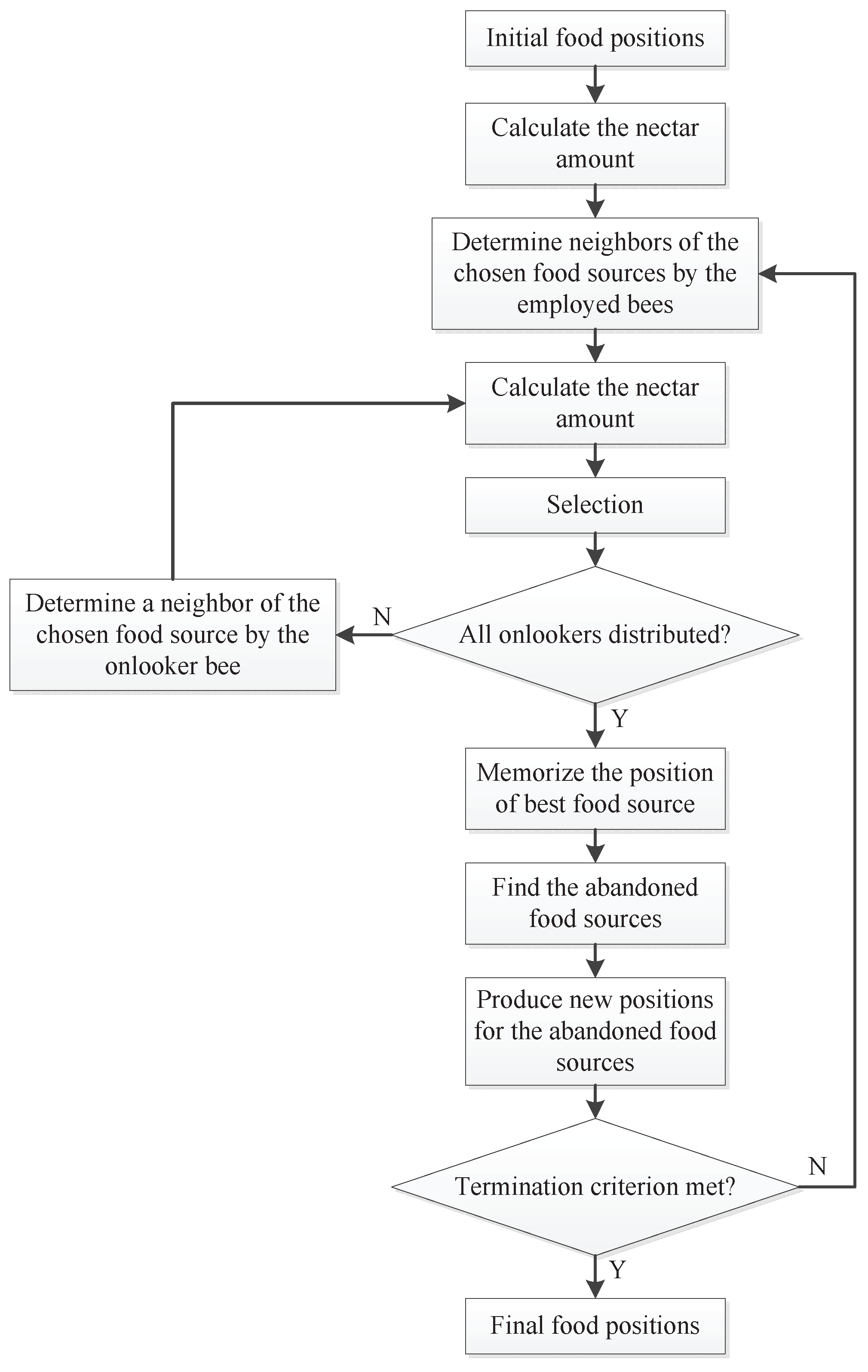
In the ABC algorithm, the artificial bees are classified into three groups: the employed bees, the onlookers and the scouts. A bee that is exploiting a food source is classified as employed. The employed bees share information with the onlooker bees, which are waiting in the hive and watching the dances of the employed bees. The onlooker bees will then choose a food source with probability proportional to the quality of that food source. Therefore, good food sources attract more bees than the bad ones. Scout bees search for new food sources randomly in the vicinity of the hive. When a scout or onlooker bee finds a food source, it becomes employed. When a food source has been fully exploited, all the employed bees associated with it will abandon the position, and may become scouts again. Therefore, scout bees perform the job of “exploration”, whereas employed and onlooker bees perform the job of “exploitation”. In the algorithm, a food source corresponds to a possible solution to the optimization problem, and the nectar amount of a food source corresponds to the fitness of the associated solution.
In ABC, the first half of the colony consist of employed bees and the other half are onlookers. The number of employed bees is equal to the number of food sources ( S N ) because it is assumed there is only one employed bee for each food source. Thus, the number of onlooker bees is also equal to the number of solutions under consideration. The ABC algorithm starts with a group of randomly generated food sources. The main procedure of ABC can be described as follows.
Step 1: 
Initialize the food sources.
Step 2: 
Each employed bee starts to work on a food source.
Step 3: 
Each onlooker bee selects a food source according to the nectar information shared by the employed.
Step 4: 
Determine the scout bees, which will search for food sources in a random manner.
Step 5: 
Test whether the termination condition is met. If not, go back to Step 2.
The detailed description for each step is given below.
(1)
The initialization phase. The S N initial solutions are randomly-generated D-dimensional real vectors. Let x i = { x i , 1 , x i , 2 , , x i , D } represent the i-th food source, which is obtained by
x i , d = x d min + r × ( x d max x d min ) , d = 1 , , D
where r is a uniform random number in the range [ 0 , 1 ] , and x d min and x d max are the lower and upper bounds for dimension d, respectively.
(2)
The employed bee phase. In this stage, each employed bee is associated with a solution. She exerts a random modification on the solution (original food source) for finding a new solution (new food source). This implements the function of neighborhood search. The new solution v i is generated from x i using a differential expression:
v i , d = x i , d + r × ( x i , d x k , d )
where d is randomly selected from { 1 , , D } , k is randomly selected from { 1 , , S N } such that k i , and r is a uniform random number in the range [ 1 , 1 ] .
Once v i is obtained, it will be evaluated and compared to x i . If the fitness of v i is better than that of x i (i.e., the nectar amount of the new food source is higher than the old one), the bee will forget the old solution and memorize the new one. Otherwise, she will keep working on x i .
(3)
The onlooker bee phase. When all employed bees have finished their local search, they share the nectar information of their food source with the onlookers, each of whom will then select a food source in a probabilistic manner. The probability p i by which an onlooker bee chooses food source x i is calculated as follows:
p i = f i i = 1 S N f i
where f i is the fitness value of x i . Obviously, the onlooker bees tend to choose the food sources with higher nectar amount.
Once the onlooker has selected a food source x i , she will also conduct a local search on x i according to Equation (2). As in the previous case, if the modified solution has a better fitness, the new solution will replace x i .
(4)
The scout bee phase. In ABC, if the quality of a solution cannot be improved after a predetermined number ( l i m i t ) of trials, the food source is assumed to be abandoned, and the corresponding employed bee becomes a scout. The scout will then produce a food source randomly by using Equation (1).
To facilitate the understanding of the algorithm, a flow chart [33] is provided as Figure 2.

4. An Estimate for the Expected Maximum Lateness

In the studied SJSSP, the objective function is expressed as an expectation because the processing times are random variables. Meanwhile, due to the NP -hardness of JSSP, there does not exist a closed-form expression to calculate the expected objective value. Therefore, the evaluation of a given schedule is not a simple task. Usually, we can utilize the idea of Monte Carlo simulation, i.e., taking the average objective value in a large number of realizations as an estimate for the expectation. However, this definitely increases the computational burden, especially when used in an optimization framework (frequent solution evaluations are needed).
If there is no strict requirement on the evaluation accuracy, it is natural to think of a time-saving strategy: cut down the number of realizations. Furthermore, if we allow only one realization of the random processing times, then a rational choice is to use the mean (expected) value of each processing time. Then, we can show the following property, that is, such an estimate is a lower bound of the true objective value.
Theorem 1. Let σ denote a feasible schedule of the considered SJSSP instance. The following inequality must hold:
E L max σ L ¯ max σ
where L max σ (random variable) is the maximum lateness corresponding to the schedule, and L ¯ max σ (constant value) is the maximum lateness in the case where each random processing time takes the value of its expectation.
Figure 2. Flow chart of the ABC algorithm.
Entropy 13 01708 g002
Proof. For the sake of simplicity, we will omit the superscript “σ” in the following proof because we are already focusing on the given schedule.
We will denote the completion time of operation O j k by c j k (a random variable). Furthermore, let t ¯ j k (resp. c ¯ j k ) denote the starting time (resp. completion time) of operation O j k when each processing time is replaced by its expected value. Since A σ is acyclic, all the operations can be sorted topologically, yielding an ordered sequence { O j k [ i ] } i = 1 n × m . In this sequence, the machine predecessors and the job predecessors of any operation O j k must be positioned before O j k . First we will prove that, for any operation O j k , E t j k t ¯ j k .
We start from the first operation ( i = 1 ) in the sequence. Because O j k [ 1 ] has no predecessor operations, we have E t j k = t ¯ j k (actually t j k = 0 ). Then, the proof procedure will continue for i = 2 , , n × m . Suppose we have already proved E t j k t ¯ j k for each operation before O j k [ i ] in the sequence, and without loss of generality, we assume that O j k [ i ] has an immediate machine predecessor O j k and an immediate job predecessor O j k , then we have
E t j k = E max c j k , c j k max E c j k , E c j k = max E t j k + p j k , E t j k + p j k max t ¯ j k + E p j k , t ¯ j k + E p j k = max c ¯ j k , c ¯ j k = t ¯ j k
where E t j k t ¯ j k and E t j k t ¯ j k hold because O j k and O j k must come before O j k in the sequence. If O j k has no job predecessor, then we set c j k = 0 in the above proof. Likewise, if O j k has no machine predecessor, then we set c j k = 0 . Therefore, the reasoning applies to each operation in the sequence.
Having proved E t j k t ¯ j k , we can now move to the objective function ( L max ). Let C ¯ j (resp. L ¯ j ) denote the completion time (resp. lateness) of job j when each random processing time takes its expected value. Meanwhile, k j represents the machine which processes the last operation of job j. Then,
E max j = 1 n { L j } max j = 1 n E L j = max j = 1 n E t j k j + p j k j d j max j = 1 n t ¯ j k j + E p j k j d j = max j = 1 n C ¯ j d j = max j = 1 n { L ¯ j }
This completes the proof of E L max σ L ¯ max σ .

5. The Proposed ABC Algorithm for Solving SJSSP

In this section, the proposed ABC is introduced in detail. First, we describe how ABC can be adapted to a discrete optimization problem like SJSSP. Second, we describe the method for comparing the quality (subject to estimation errors) of different solutions in the proposed ABC. Since the problem is stochastic, in the solution comparison process, we must decide how to allocate the available simulation replications. This problem is resolved by the model proposed in the third subsection. Finally, to facilitate the utilization of the simulation allocation model, we slightly revise the implementation of the local search procedure in standard ABC.

5.1. Adaptation to the Discrete Problem

Since the standard ABC is intended for continuous function optimization, we need to introduce some modifications in order to adapt it to SJSSP.

5.1.1. Encoding and Decoding

First, the encoding scheme for SJSSP is based on operation sequences instead of real number vectors. In particular, each solution (food source) is represented by a sequence of n × m operations, which can be transformed into a feasible schedule by the “schedule builder” presented below. This procedure functions by iteratively scanning the sequence and then picking out the first schedulable operation [34] in the sequence. In order to build an active schedule, each operation is inserted into the earliest possible idle period (i.e., time interval not occupied by the previously scheduled operations).
Input: A sequence of operations, π, with a length of n × m .
Step 1: 
Let σ be an empty matrix of size m × n .
Step 2: 
If π = , output σ (and the corresponding L max if necessary) and terminate the procedure. Otherwise, continue the following steps.
Step 3: 
Find the first schedulable operation in the sequence π, denoted by O * .
Step 4: 
Identify the machine required to process O * and denote it by k * . Record the expected processing time of O * as p * .
Step 5: 
Schedule the operation O * :
(5.1)
Scan the Gantt chart of machine k * (which records the processing information of the already scheduled operations) from time zero and test whether O * can be inserted into each idle period [ a , b ] , i.e., whether the following condition is met: max { a , C J P * } + p * b (where C J P * denotes the completion time of the immediate job predecessor of operation O * ).
(5.2)
If the above inequality is satisfied for the idle interval between operation o 1 and o 2 on machine k * , then insert O * between o 1 and o 2 in the k * -th row of σ. Otherwise (no idle intervals can hold O * ), insert it at the back of the k * -th row of σ. Update the Gantt chart records for the starting time and completion time of operation O * .
Step 6: 
Delete operation O * from π. Go back to Step 2.

5.1.2. Initialization

Second, the solution initialization policy (Equation (1) in standard ABC) should be modified to comply with the solution encoding scheme. Here we use the famous ATC (apparent tardiness cost) rule [35] to produce the initial population. To generate the u-th solution, we first make a sample of the random processing times according to their distributions, denoted as { p j k ( u ) } . Then, the ATC rule is applied in a simulation-based scheduling procedure, where the operation with the largest Z j k value will be selected for processing when a machine is freed at time t.
Z j k ( t ) = w j p j k ( u ) · exp d j t p j k ( u ) O j k J S ( O j k ) W ^ j k + p j k ( u ) + K · p ¯ ( u )
where J S ( O j k ) is the set of job successors of operation O j k . p ¯ ( u ) denotes the average processing time of the currently waiting operations in the machine’s buffer. K is a scaling parameter (or called “look-ahead” parameter). W ^ j k is the estimated lead time of operation O j k . Here it is assumed K = 2 and W ^ j k = 0 . 4 p j k ( u ) .

5.1.3. Neighborhood Structure

Third, the neighborhood search mechanism (Equation (2) in standard ABC) also needs to be modified accordingly. Let’s recall that, in the case of deterministic JSSP, we must focus on the operations that belong to the blocks [36] of tardy jobs in order to improve the current solution. Therefore, the neighborhood search for SJSSP can be performed by using the expected values of processing times to determine the critical paths and blocks. Particularly, we first select two adjacent operations randomly from a block related with a tardy job, and then the SWAP operator is applied to exchange the positions of these two operations in the encoded solution.

5.2. The Comparison of Solutions

In order to approximate E L max σ , we need to implement the schedule σ under different realizations of the random processing times. When σ has been evaluated for a sufficient number of times, say τ, then its objective value can be approximated by 1 τ i = 1 τ L max σ ( i ) (where L max σ ( i ) corresponds to the i-th realization). This is consistent with the idea of Monte Carlo simulation.
In the employed bee phase and the onlooker bee phase, the newly-generated solution must be compared with the original solution in order to determine which one should be kept. For deterministic optimization problems, this can be done by simply comparing the exact objective values of the two solutions. But in the stochastic case, the comparisons may not be so straightforward because we can only obtain approximated (noisy) objective values as mentioned above. In this study, we will utilize the following two mechanisms for comparison purposes.
(I) Pre-screening. Because L ¯ max σ is a lower bound for E L max σ (Theorem 1), we can arrive at the following conclusion which is useful for the pre-screening of candidate solutions.
Corollary 1. For two candidate solutions x 1 (the equivalent schedule is denoted by σ 1 ) and x 2 (the equivalent schedule is denoted by σ 2 ), if L ¯ max σ 2 E L max σ 1 , then x 2 must be inferior to x 1 and thus need not be considered.
(II) Hypothesis test. If the candidate solution has passed the pre-screening, then hypothesis test is used for comparing the quality of the two solutions.
Suppose we have implemented n i simulation replications for solution x i whose true objective value is f x i = E L max σ i ( i = 1 , 2 ). Then, the sample mean and sample variance can be calculated by
f ¯ i = 1 n i j = 1 n i f i ( j ) s i 2 = 1 n i 1 j = 1 n i f i ( j ) f ¯ i 2
where f i ( j ) is the objective value obtained in the j-th simulation replication for solution x i .
Let the null hypothesis H 0 be “ f x 1 = f x 2 ”, and thus the alternative hypothesis H 1 is “ f x 1 f x 2 ”. According to the statistical theory, the critical region of H 0 is
f ¯ 1 f ¯ 2 Z = z α / 2 s 1 2 n 1 + s 2 2 n 2
where z α / 2 is the value such that the area to its right under the standard normal curve is exactly α / 2 . Therefore, if f ¯ 1 f ¯ 2 < Z (i.e., the null hypothesis holds), it is said that there exists no statistical difference between x 1 and x 2 . Otherwise, if f ¯ 1 f ¯ 2 Z , x 2 is statistically better than x 1 ; if f ¯ 1 f ¯ 2 Z , x 1 is statistically better than x 2 .

5.3. The Allocation of Simulation Replications

In the previous subsection, we assume that n i simulation replications have been performed for solution x i before the hypothesis test. But how should the value of n i be determined? We know that full-length simulation is very time-consuming, so a smaller value is desirable for n i . On the other hand, however, if n i is too small, the approximation for the objective values will be over-imprecise, which can mislead the hypothesis test. To achieve a balance, here we borrow an idea from the solution to the famous K-armed bandit problem.
The K-armed bandit problem can be described as K random variables, X i ( 1 i K ), where X i represents the stochastic reward given by the i-th gambling machine. The distributions of X i are independent but generally not identical. The laws of the distributions and the expectations μ i for the rewards X i are unknown. The goal is to find a strategy that determines the next machine to play (based on the past plays and the received rewards) that maximizes the expected total reward for the player.
Since a player does not know which of the machines is the best, he can only guess the reward distributions from successive plays. Clearly, he has to make a trade-off between the following two choices:
  • The player tends to concentrate his efforts on the machines that gave the highest rewards in the past plays. Intuitively, this choice will maximize the potential gains.
  • The player also wants to try the machines which he has played very few times in the past. The reward distributions of these machines are quite unclear, but it is likely that they provide even higher rewards.
Therefore, it is necessary to strike a wise balance between exploiting the currently best machine and exploring the other machines to make sure that none of those is even better.
When allocating the simulation replications, we are actually facing a similar situation. There are a number of solutions waiting to be evaluated. For each solution, the objective value obtained from one simulation is a random variable following an unknown distribution. We want to find out the quality of these solutions with the minimum total number of simulation replications. The question is to decide which solution should get the next chance of simulation. Obviously, the solutions are analogous to the gambling machines, and the simulations are analogous to the gambler’s tries.
Here we use an algorithm called UCB1 [38] for making the allocation decisions. If the number of candidate solutions is K, while the available computing resource is only enough to support a total of T replications of simulation ( T > δ K , where δ is the number of replications assigned at a time), then the algorithm can be adapted to our problem as follows.
Input: A set of K candidate solutions.
Step 1: 
Perform δ simulation replications for each solution x k . Denote the mean objective value by f ¯ k , and denote the standard deviation by s k . Calculate the estimated “reward” as r ˜ k = s k / f ¯ k . Set ν k = δ ( k = 1 , , K ) and ν = δ K .
Step 2: 
Calculate a priority index for each solution x k : ρ k = r ˜ k + 2 ln ν ν k .
Step 3: 
Perform δ additional simulation replications for the solution x k * with the maximum ρ value. Update f ¯ k * , s k * and r ˜ k * for this solution. Let ν k * ν k * + δ and ν ν + δ .
Step 4: 
If ν < T , go back to Step 2. Otherwise, terminate the procedure.
In the adapted UCB1 (noted as A-UCB1) algorithm, ν k records the number of times that solution x k has been evaluated through simulation, while ν is the total number of simulation replications that have been assigned so far. The “reward” from trying x k is defined as the relative standard deviation of the simulated objective values. Under the effect of ρ, the definition of r k ensures that the simulation replications tend to be allocated to the solutions whose quality is still unclear (represented by the relatively large s k ). Meanwhile, the algorithm will also allocate simulation replications to the solutions which have been evaluated very few times (represented by the small ν k ). In sum, the A-UCB1 algorithm aims at promoting the computational efficiency in the evaluation of solutions. Based on extensive computational tests, the value of δ is set as T / 100 .

5.4. Revised Implementation of the Local Search in ABC

In the employed bee phase and the onlooker bee phase, the artificial bees are actually performing the local search task. Considering the special features of the stochastic optimization problem, we slightly modify the implementation of this local search mechanism. In particular, we evaluate and compare the solutions group by group rather than one by one. The aim is to utilize the benefits of the A-UCB1 algorithm (for controlling the computational burden) and the hypothesis test (for increasing the diversity of the whole population). Our implementation is detailed as follows. Suppose the bees are already associated with each solution.
Step 1: 
Use A-UCB1 to allocate a total of T simulation replications to the solutions in the current population P. Save the estimated mean objective value and variance for each solution.
Step 2: 
Generate a new solution based on each original solution using the SWAP operator. Apply the pre-screening method (Corollary 1) to ensure the quality of each new solution [39]. Denote the set of new solutions by P new .
Step 3: 
Use A-UCB1 to allocate a total of T simulation replications to the solutions in P new . Save the estimated mean objective value and variance for each solution.
Step 4: 
Perform hypothesis tests to determine the new population: 0pt
(4.1)
Sort all the solutions in P P new in non-decreasing order of the estimated objective values, yielding a sequence { x [ 1 ] , , x [ 2 S N ] } . Put x [ 1 ] into the ultimate population P * . Let i = 1 , j = 2 .
(4.2)
Perform hypothesis test for x [ j ] and the i-th solution (the latest) in P * . If the null hypothesis holds, x [ j ] is rejected. Otherwise, x [ j ] is appended to P * and let i i + 1 .
(4.3)
If i < S N and j < 2 S N , then let j j + 1 and go to Step 4.2. Otherwise, go to Step 4.4.
(4.4)
If i = S N , the ultimate population has been determined. Otherwise, generate ( S N i ) new solutions randomly, evaluate them (each one is evaluated with T / S N simulation replications) and append them to P * .
Step 5: 
Compare P * with P and check whether each new solution has been accepted (i.e., in P * ). If accepted, let the corresponding bee fly to the new solution.
In the proposed ABC algorithm, the above procedure is used in place of the one-to-one greedy selection policy in standard ABC. This is in consideration of the specific features of stochastic optimization. Evaluating a group of solutions together is beneficial, because A-UCB1 will allocate more simulation replications to good solutions (with smaller f ¯ k ) to make sure about their true performance and avoid wasting time on inferior solutions (with larger f ¯ k ). The hypothesis test is used for maintaining an adequate level of diversity of the solution population. In Step 4.2, if x [ j ] does not significantly differ from the most recent solution in P * , it will not have a chance to enter P * . Finally, if the number of qualified solutions is less than S N , the rest of solutions will be generated randomly.

6. The Computational Experiments

6.1. Generation of Test Instances

To test the effectiveness of the proposed algorithm, computational experiments are conducted on a number of randomly-generated test instances. In each instance, the route of each job is a random permutation of m machines. Three types of distribution patterns are considered for the random processing times: normal distribution, uniform distribution and exponential distribution. In all cases, the mean values ( μ j k ) are generated from the uniform distribution U 1 , 99 . In the case of normal distributions (i.e., p j k N ( μ j k , σ j k 2 ) ), the standard deviation is controlled by σ j k = θ × μ j k (θ describes the level of variability). In the case of uniform distributions (i.e., p j k U ( μ j k ω j k , μ j k + ω j k ) ), the width parameter is given by ω j k = θ × μ j k . In the case of exponential distributions (i.e., p j k Exp ( λ j k ) ), the only parameter is given by λ j k = 1 / μ j k . The due dates are obtained by a series of simulation runs which apply different priority rules (such as SPT, EDD, etc.) on each machine, and the due date of each job is finally set as its average completion time. This method can generate reasonably tight due dates. Meanwhile, the weight of each job is generated from the uniform distribution U 1 , 10 . The following computational experiments are conducted in Visual C++ 2010 on an Intel Corei5-750/3GB RAM/Windows 7 PC.

6.2. The Computational Results and Comparisons

Based on extensive computational tests (not listed due to space limitations), the settings of key parameters in the final ABC algorithm are: S N = 30 , l i m i t = 40 and T = 1000 (for each evaluation). The confidence level for the hypothesis test is α = 0 . 05 .
In the following, we will use the proposed ABC to solve different-sized SJSSP instances. The results are compared with the hybrid optimization method PSO-SA [40], which utilizes SA (simulated annealing) as a local optimizer for PSO. In order to make the comparisons meaningful, we set a computational time limit for both algorithms. Normally, the time limit should be set according to the size of the instance. In our experiment, the time limit for solving a n × m instance is determined as t = 0 . 2 × ( n × m ) . For example, the allowed computational time for a 20 × 10 instance is 40 sec. Each algorithm is run for 20 independent times on each SJSSP instance.
We report the best, average and worst objective values (exact evaluation [41] for the output solutions) in the 20 runs. Table 1, Table 2 and Table 3 report the results under normal distributions, Table 4, Table 5 and Table 6 report the results under uniform distributions, and Table 7 reports the results under exponential distributions.
Table 1. The computational results under normal distributions with θ = 0 . 1 .
Size
n × m
Instance
No.
ABCPSO-SA
bestaverageworstbestaverageworst
10 × 10 146.152.158.050.553.259.8
247.449.153.246.753.154.8
350.051.754.050.452.354.9
456.261.862.760.862.566.2
550.956.061.353.556.361.1
20 × 10 666.069.075.370.375.886.1
763.067.671.667.072.183.8
861.865.567.565.070.975.8
964.970.074.969.476.778.2
1060.568.770.064.070.576.1
20 × 15 1180.683.184.185.186.288.2
1280.984.889.286.187.890.9
1367.172.583.275.777.084.5
1477.481.885.679.183.789.3
1572.378.683.674.981.886.6
20 × 20 1699.9106.9121.2103.5111.0124.7
1797.4103.2118.2114.9128.0134.9
18104.6114.9123.8120.8129.8137.1
19111.4117.5120.3120.7123.9131.6
2098.5115.2121.4121.5128.6132.7
In addition, we have also performed Mann–Whitney U tests to statistically compare the computational results. Because each algorithm is run for 20 times, we have n 1 = n 2 = 20 in the Mann–Whitney U test. The null hypothesis is that there is no difference between the results of the two compared algorithms. Therefore, if the obtained U (the lesser of U 1 and U 2 ) is below 127, the null hypothesis can be rejected at the 5% level. Furthermore, if U < 105 , the null can be rejected at the 1% level. The values of U are listed in Table 8.
Table 2. The computational results under normal distributions with θ = 0 . 2 .
Size
n × m
Instance
No.
ABCPSO-SA
bestaverageworstbestaverageworst
10 × 10 151.162.767.860.063.368.5
253.155.660.654.960.264.9
354.357.560.858.060.166.1
463.870.775.470.074.280.6
559.062.769.063.566.569.5
20 × 10 667.172.676.173.381.193.0
764.269.471.372.175.886.6
864.666.969.864.273.178.9
964.672.174.773.980.682.3
1061.168.471.267.273.982.2
20 × 15 1184.087.690.184.690.694.1
1286.591.593.296.798.6103.8
1374.280.390.881.087.396.7
1484.888.890.785.191.298.8
1579.483.990.985.389.294.4
20 × 20 16111.3117.5133.5115.4122.7137.3
17100.2108.8127.6127.1131.1148.9
18110.9118.1126.9127.3138.4146.8
19118.5123.7129.2131.5139.2143.6
20101.7122.2130.0128.7136.7140.8
Table 3. The computational results under normal distributions with θ = 0 . 3 .
Size
n × m
Instance
No.
ABCPSO-SA
bestaverageworstbestaverageworst
10 × 10 153.467.469.160.667.573.3
256.060.063.156.566.168.6
360.261.965.162.563.569.6
469.172.874.574.777.882.5
560.967.771.766.070.171.1
20 × 10 674.377.381.481.886.8100.5
770.875.881.677.180.695.6
869.370.474.570.979.288.1
972.076.581.977.687.590.4
1066.577.978.971.880.085.5
20 × 15 1191.292.696.087.495.299.8
1290.594.698.9101.0104.6105.7
1376.183.295.087.189.898.6
1488.691.797.886.393.199.1
1579.788.692.085.992.899.4
20 × 20 16116.5120.3131.1115.3124.4140.1
17104.4111.2130.9128.6146.3151.2
18114.8121.7134.5140.7151.3157.3
19121.3125.7131.3133.7137.6147.0
20105.8126.5133.8139.1145.7152.6
Table 4. The computational results under uniform distributions with θ = 0 . 1 .
Size
n × m
Instance
No.
ABCPSO-SA
bestaverageworstbestaverageworst
10 × 10 138.041.947.540.844.750.4
238.941.044.439.144.446.7
341.642.745.640.642.745.1
446.251.753.248.752.154.5
541.646.551.443.545.851.4
20 × 10 655.858.664.759.663.271.3
751.458.159.654.459.868.9
852.953.755.153.057.662.0
954.758.860.159.161.864.2
1050.757.259.053.559.064.3
20 × 15 1165.868.471.667.270.273.9
1267.070.375.369.173.076.8
1356.758.466.761.062.471.7
1462.367.770.664.168.975.8
1560.267.369.062.666.670.5
20 × 20 1680.186.9103.488.493.3106.9
1782.888.1100.897.1104.0115.6
1886.595.9105.699.1108.2115.4
1989.396.998.7101.8106.2108.3
2083.292.5103.7103.3107.0110.9
Table 5. The computational results under uniform distributions with θ = 0 . 2 .
Size
n × m
Instance
No.
ABCPSO-SA
bestaverageworstbestaverageworst
10 × 10 142.554.659.451.054.060.1
244.646.652.146.453.354.6
347.849.752.351.052.258.0
454.262.567.158.964.767.7
551.853.058.556.358.560.7
20 × 10 658.464.367.364.771.482.2
754.960.163.361.666.872.4
854.857.659.753.964.265.9
956.561.967.262.470.572.1
1053.061.262.956.663.669.9
20 × 15 1171.575.877.974.579.981.5
1277.080.084.284.487.290.9
1365.670.579.969.173.882.8
1472.678.885.071.677.387.5
1567.870.679.273.577.881.2
20 × 20 1695.698.5113.0101.0105.7114.8
1783.490.7111.599.4109.5130.4
1893.998.9108.0112.2121.1125.9
1999.9102.8109.3115.0119.2120.4
2086.9102.0111.4108.4117.3120.6
Table 6. The computational results under uniform distributions with θ = 0 . 3 .
Size
n × m
Instance
No.
ABCPSO-SA
bestaverageworstbestaverageworst
10 × 10 148.158.460.452.561.063.3
251.252.254.548.758.261.3
353.255.658.756.658.361.8
460.963.065.666.767.974.2
555.060.062.759.561.563.9
20 × 10 667.969.470.875.278.987.4
761.168.973.568.871.784.8
860.263.266.264.871.478.7
963.566.173.168.078.179.3
1057.969.272.064.571.576.0
20 × 15 1179.581.885.781.485.490.4
1283.285.590.290.792.395.6
1367.976.186.475.780.588.2
1478.680.387.079.585.389.9
1571.679.181.074.081.590.9
20 × 20 16101.3107.2113.2102.5110.2127.3
1793.0100.0116.8111.6126.5139.0
18101.0105.4122.2129.3132.1143.9
19108.9110.3114.8122.4125.6133.0
2091.9115.5121.5122.1127.7139.3
Table 7. The computational results under exponential distributions
Size
n × m
Instance
No.
ABCPSO-SA
bestaverageworstbestaverageworst
10 × 10 185.6109.6114.3100.8109.4118.2
291.3100.2102.093.3109.4114.1
396.198.3108.3103.1104.3111.5
4114.4121.0129.7123.3128.5132.1
5101.1111.4119.9106.2115.7117.7
20 × 10 6123.7126.8131.9135.2145.8161.8
7113.8124.8134.2124.6134.9154.3
8113.3116.2123.0116.2130.2143.2
9116.6125.7132.7130.3146.4147.6
10107.9126.1131.4117.6131.3141.9
20 × 15 11141.5149.4156.9146.0157.0160.2
12148.8153.4162.4167.5175.2177.0
13122.8139.3159.5142.9146.8158.3
14143.7150.5160.7144.5149.8163.6
15129.3146.8150.0138.2149.7164.9
20 × 20 16193.8199.8215.2192.4202.4229.1
17168.0184.4217.6213.0242.9251.8
18185.7196.2215.7226.8242.4251.9
19199.6209.5213.6214.6225.0241.9
20170.2209.2221.0228.5240.0249.9
Table 8. Mann–Whitney U tests on the computational results.
Instance No.NormalUniformExponential
θ = 0 . 2 θ = 0 . 3 θ = 0 . 1 θ = 0 . 2 θ = 0 . 3
197948299978676
293857994897870
395847994878076
487787090797268
590807989817872
680746883766962
782786984786964
884797086797366
979716478726361
1081746783736564
1186817485817670
1291867990867870
1393797790798173
1488878491888682
1596847894898173
1688777089767064
1777686074706359
1870665972646155
1980676684666661
2069646070646253
Based on the statistical tests, we can conclude that ABC is significantly more effective than the comparative method. In addition, the following comments can be made.
(1)
According to the tables, the advantage of ABC over PSO-SA is greater when the variability level of processing times is higher (represented by larger θ or the case of exponential distribution). This can be attributed to the function of A-UCB1, which is responsible for the allocation of the limited computational resources. If θ is small, the objective value of a solution can be obtained with only a few replications. In this case, the A-UCB1 strategy is not significantly better than an equal allocation of the available replications (the case of PSO-SA). However, when the variability increases, the computational time becomes a relatively scarce resource. In order to correctly identify high-quality solutions, the limited replications should be allocated in an efficient manner rather than evenly. So in this case, the advantage of using A-UCB1 becomes evident.
(2)
According to the tables, ABC outperforms PSO-SA to a greater extent when solving the larger-scale instances. If the solution space is huge, PSO must rely on the additional local search module (SA) to promote the searching efficiency. However, SA is not so efficient as the inherent local search mechanism (employed and onlooker bees) in ABC, especially under tight time budgets. From another perspective, ABC systematically combines the exploration and exploitation abilities, and thus it works in a coordinated fashion. By contrast, the hybrid algorithm uses PSO for exploration and SA for exploitation, but the two algorithms have different search patterns. This may weaken the cooperation between PSO and SA in solving large-scale SJSSP. Therefore, ABC alone is more efficient than the hybrid algorithm.

7. Conclusions

In this paper, an artificial bee colony algorithm is proposed for solving the job shop scheduling problem with random processing times. The objective function is to minimize the expected maximum lateness. In view of the stochastic nature of the problem, two mechanisms are devised for the evaluation of solutions. First, a quick-and-dirty performance estimate is used to pre-screen the candidate solutions, so that the obviously inferior solutions can be eliminated at an early stage. Then, Monte Carlo simulation is applied to obtain a more accurate evaluation for the surviving solutions. In this process, a simulation budget allocation method is designed based on the K-armed bandit metaphor. This helps to utilize the limited computational time in an efficient manner. The computational results on a wide range of test instances reveal the superiority of the proposed approach.
The future research can be conducted from the following aspects:
(1)
It is worthwhile to consider other types of randomness in job shops, for example, the uncertainty in the processing routes of certain jobs.
(2)
It is worthwhile to investigate the method for discovering and utilizing problem-specific characteristics of SJSSP. This will make the ABC algorithm more pertinent to this problem.

Acknowledgment

This work is supported by the National Natural Science Foundation of China under Grant Nos. 61104176, 60874071. We would express our thanks to the two anonymous referees for their pertinent comments that help to improve the paper.

References and Notes

  1. Lenstra, J.K.; Kan, A.H.G.R.; Brucker, P. Complexity of machine scheduling problems. Ann. Discret. Math. 1977, 1, 343–362. [Google Scholar]
  2. Pezzella, F.; Morganti, G.; Ciaschetti, G. A genetic algorithm for the flexible job-shop scheduling problem. Comput. Oper. Res. 2008, 35, 3202–3212. [Google Scholar] [CrossRef]
  3. Chen, S.H.; Chen, M.C.; Chang, P.C.; Chen, Y.M. EA/G-GA for single machine scheduling problems with earliness/tardiness costs. Entropy 2011, 13, 1152–1169. [Google Scholar] [CrossRef]
  4. Nowicki, E.; Smutnicki, C. An advanced tabu search algorithm for the job shop problem. J. Sched. 2005, 8, 145–159. [Google Scholar] [CrossRef]
  5. Lei, D. Pareto archive particle swarm optimization for multi-objective fuzzy job shop scheduling problems. Int. J. Adv. Manuf. Technol. 2008, 37, 157–165. [Google Scholar] [CrossRef]
  6. Rossi, A.; Dini, G. Flexible job-shop scheduling with routing flexibility and separable setup times using ant colony optimisation method. Robot. Comput. Integr. Manuf. 2007, 23, 503–516. [Google Scholar] [CrossRef]
  7. Li, J.; Pan, Q.; Xie, S.; Wang, S. A hybrid artificial bee colony algorithm for flexible job shop scheduling problems. Int. J. Comput. Commun. Control 2011, 6, 286–296. [Google Scholar]
  8. Yoshitomi, Y. A genetic algorithm approach to solving stochastic job-shop scheduling problems. Int. Trans. Oper. Res. 2002, 9, 479–495. [Google Scholar] [CrossRef]
  9. Yoshitomi, Y.; Yamaguchi, R. A genetic algorithm and the Monte Carlo method for stochastic job-shop scheduling. Int. Trans. Oper. Res. 2003, 10, 577–596. [Google Scholar] [CrossRef]
  10. Golenko-Ginzburg, D.; Gonik, A. Optimal job-shop scheduling with random operations and cost objectives. Int. J. Prod. Econ. 2002, 76, 147–157. [Google Scholar] [CrossRef]
  11. Tavakkoli-Moghaddam, R.; Jolai, F.; Vaziri, F.; Ahmed, P.K.; Azaron, A. A hybrid method for solving stochastic job shop scheduling problems. Appl. Math. Comput. 2005, 170, 185–206. [Google Scholar] [CrossRef]
  12. Luh, P.; Chen, D.; Thakur, L. An effective approach for job-shop scheduling with uncertain processing requirements. IEEE Trans. Robot. Autom. 1999, 15, 328–339. [Google Scholar] [CrossRef]
  13. Lai, T.; Sotskov, Y.; Sotskova, N.; Werner, F. Mean flow time minimization with given bounds of processing times. Eur. J. Oper. Res. 2004, 159, 558–573. [Google Scholar] [CrossRef]
  14. Singer, M. Forecasting policies for scheduling a stochastic due date job shop. Int. J. Prod. Res. 2000, 38, 3623–3637. [Google Scholar] [CrossRef]
  15. Lei, D. Scheduling stochastic job shop subject to random breakdown to minimize makespan. Int. J. Adv. Manuf. Technol. 2011, 55, 1183–1192. [Google Scholar] [CrossRef]
  16. Lei, D. Simplified multi-objective genetic algorithms for stochastic job shop scheduling. Appl. Soft Comput. 2011. [Google Scholar] [CrossRef]
  17. Gu, J.; Gu, X.; Gu, M. A novel parallel quantum genetic algorithm for stochastic job shop scheduling. J. Math. Anal. Appl. 2009, 355, 63–81. [Google Scholar] [CrossRef]
  18. Gu, J.; Gu, M.; Cao, C.; Gu, X. A novel competitive co-evolutionary quantum genetic algorithm for stochastic job shop scheduling problem. Comput. Oper. Res. 2010, 37, 927–937. [Google Scholar] [CrossRef]
  19. Mahdavi, I.; Shirazi, B.; Solimanpur, M. Development of a simulation-based decision support system for controlling stochastic flexible job shop manufacturing systems. Simul. Model. Pract. Theory 2010, 18, 768–786. [Google Scholar] [CrossRef]
  20. Azadeh, A.; Negahban, A.; Moghaddam, M. A hybrid computer simulation-artificial neural network algorithm for optimisation of dispatching rule selection in stochastic job shop scheduling problems. Int. J. Prod. Res. 2011. [Google Scholar] [CrossRef]
  21. Bianchi, L.; Dorigo, M.; Gambardella, L.; Gutjahr, W. A survey on metaheuristics for stochastic combinatorial optimization. Nat. Comput. 2009, 8, 239–287. [Google Scholar] [CrossRef]
  22. Karaboga, D.; Akay, B. A survey: algorithms simulating bee swarm intelligence. Artif. Intell. Rev. 2009, 31, 61–85. [Google Scholar] [CrossRef]
  23. Karaboga, D. An Idea Based on Honey Bee Swarm for Numerical Optimization; Technical Report for Computer Engineering Department, Erciyes University: Kayseri, Turkey, October 2005. [Google Scholar]
  24. Karaboga, D.; Basturk, B. On the performance of artificial bee colony (ABC) algorithm. Appl. Soft Comput. 2008, 8, 687–697. [Google Scholar] [CrossRef]
  25. Karaboga, D.; Akay, B. A comparative study of artificial bee colony algorithm. Appl. Math. Comput. 2009, 214, 108–132. [Google Scholar] [CrossRef]
  26. Karaboga, D.; Basturk, B. A powerful and efficient algorithm for numerical function optimization: artificial bee colony (ABC) algorithm. J. Glob. Optim. 2007, 39, 459–471. [Google Scholar] [CrossRef]
  27. Kang, F.; Li, J.; Xu, Q. Structural inverse analysis by hybrid simplex artificial bee colony algorithms. Comput. Struct. 2009, 87, 861–870. [Google Scholar] [CrossRef]
  28. Sonmez, M. Discrete optimum design of truss structures using artificial bee colony algorithm. Struct. Multidiscip. Optim. 2011, 43, 85–97. [Google Scholar] [CrossRef]
  29. Samanta, S.; Chakraborty, S. Parametric optimization of some non-traditional machining processes using artificial bee colony algorithm. Eng. Appl. Artif. Intell. 2011, 24, 946–957. [Google Scholar] [CrossRef]
  30. Huang, Y.; Lin, J. A new bee colony optimization algorithm with idle-time-based filtering scheme for open shop-scheduling problems. Expert Syst. Appl. 2011, 38, 5438–5447. [Google Scholar] [CrossRef]
  31. Jain, A.S.; Meeran, S. Deterministic job-shop scheduling: past, present and future. Eur. J. Oper. Res. 1999, 113, 390–434. [Google Scholar] [CrossRef]
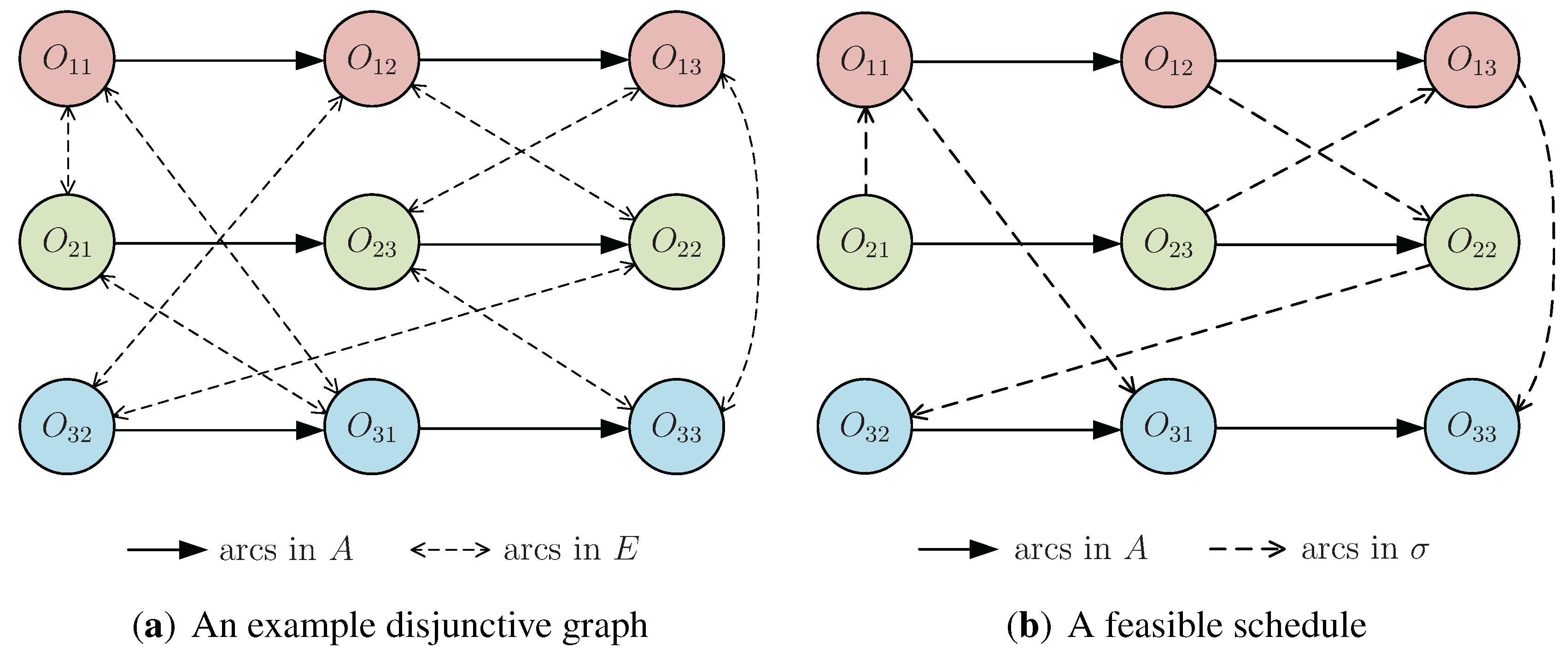
  32. In the rest of the paper, we do not distinguish between σ and the schedule. For the convenience of expression, we will write σ as a matrix. The k-th row of σ represents the processing order of the operations on machine k.
  33. Akay, B.; Karaboga, D. Artificial bee colony algorithm for large-scale problems and engineering design optimization. J. Intell. Manuf. 2011. [Google Scholar] [CrossRef]
  34. An operation is schedulable if its immediate job predecessor has already been scheduled or if it is the first operation of a certain job.
  35. Vepsalainen, A.P.; Morton, T.E. Priority rules for job shops with weighted tardy costs. Manag. Sci. 1987, 33, 1035–1047. [Google Scholar] [CrossRef]
  36. A sequence of operations in the critical path is called a block if (1) it contains at least two operations and (2) the sequence includes a maximum number of operations that are consecutively processed by the same machine [37].
  37. Pinedo, M. Scheduling: Theory, Algorithms and Systems, 3rd ed.; Springer: New York, NY, USA, 2008. [Google Scholar]
  38. Auer, P.; Cesa-Bianchi, N.; Fischer, P. Finite-time analysis of the multiarmed bandit problem. Mach. Learn. 2002, 47, 235–256. [Google Scholar] [CrossRef]
  39. If a newly-generated solution does not pass the pre-screening test, then simply generate another solution from the neighborhood, and so on.
  40. Liu, B.; Wang, L.; Jin, Y.H. Hybrid Particle Swarm Optimization for Flow Shop Scheduling with Stochastic Processing Time. In Lecture Notes in Computer Science; Springer: Berlin, Heidelberg, Germany, 2005; Volume 3801, pp. 630–637. [Google Scholar]
  41. The mean value resulted from 1000 simulation replications (which is large enough for the considered test instances) is regarded as the exact evaluation of a solution.

