Application of the EGM Method to a LED-Based Spotlight: A Constrained Pseudo-Optimization Design Process Based on the Analysis of the Local Entropy Generation Maps

Abstract

In this paper, the entropy generation minimization (EGM) method is applied to an industrial heat transfer problem: the forced convective cooling of a LED-based spotlight. The design specification calls for eighteen diodes arranged on a circular copper plate of 35 mm diameter. Every diode dissipates 3 W and the maximum allowed temperature of the plate is 80 °C. The cooling relies on the forced convection driven by a jet of air impinging on the plate. An initial complex geometry of plate fins is presented and analyzed with a commercial CFD code that computes the entropy generation rate. A pseudo-optimization process is carried out via a successive series of design modifications based on a careful analysis of the entropy generation maps. One of the advantages of the EGM method is that the rationale behind each step of the design process can be justified on a physical basis. It is found that the best performance is attained when the fins are periodically spaced in the radial direction.

1. Introduction

A fundamental thermodynamic theorem states that for whatever open process whose evolution can be approximated as a succession of quasi-equilibrium states and working in thermal contact with an ambient at T₀, the lost available power |${\dot{\mathit{W}}}_{\mathit{r}\mathit{e}\mathit{v}}-\dot{\mathit{W}}$|, i.e., the difference between the ideally produced or absorbed power and the one really extracted, is proportional to the global rate of entropy generation ${\dot{S}}_{gen}$: ${\dot{\mathit{W}}}_{\mathit{r}\mathit{e}\mathit{v}}-\dot{\mathit{W}}={\mathit{T}}_{\mathit{0}}\cdot {\dot{\mathit{S}}}_{\mathit{g}\mathit{e}\mathit{n}}$ [1]. The lost power (${\dot{W}}_{rev}-\dot{W}$) is always positive, regardless of whether the system is a power producer (e.g., an expander) or a power user (e.g., a compressor). Although not often exploited in real design applications, this theorem is of the utmost importance for the designer, in that it allows for a direct comparison of different configurations (“design options”) that either produce the same output with less irreversible losses or use the same amount of resource input to generate a larger output; both cases corresponding of course to a higher resource-to-end use efficiency. Naturally, the minimization of the entropy generation is not an easy task in practical cases, especially when complicated boundary conditions apply and/or when the operating point is varying in time. During the last three decades the Entropy Generation Minimization (EGM) method has become a well-established procedure in thermal science and engineering. The method relies on the simultaneous application of the heat transfer and engineering thermodynamics principles, in pursuit of realistic models for heat transfer processes, devices and installations. The overwhelming majority of applications of the method for heat transfer problems employs lumped-sum parameter models: the global rate of entropy generation (${\dot{S}}_{gen}$ [W/K]) is analytically expressed as a function of the topology and physical characteristics of the system (critical dimension, materials...) using correlations for average heat transfer rates and fluid friction available in literature. Then, by varying one or more of the design variables which ${\dot{S}}_{gen}$ depends upon, a minimum of the function ${\dot{S}}_{gen}$ is sought after; thence, an optimal geometry is determined. Many examples of this lumped-sum parameter model technique applied to fundamental heat transfer problems are presented in [1,2,3,4,5]. Pin-fins geometries are optimized with this method in [6,7], while plate-fins heat sinks are optimized in [8,9]. The key point of this deterministic approach is the analytical definition of ${\dot{S}}_{gen}$ as a function of critical design parameters, like geometry and working conditions. This function has to be inferred with the simultaneous application of principles of heat and mass transfer, fluid mechanics and engineering thermodynamics. Its ability to well describe the inherent irreversibility of the engineering system is closely linked to the “quality” of the correlations on which it relies. But, once we are able to actually write a semi-empirical analytic functional for ${\dot{S}}_{gen}$, finding its minimum is more a mathematical than a physical problem. One of the aims of the present work is to describe a different, heuristic, approach: the initial configuration is successively improved by introducing design changes based on a careful analysis of the local entropy generation maps obtained by means of Computational Fluid Dynamics (CFD) simulations. One of the advantages of this approach is that the rationale behind each step of the design process can be justified on a physical basis. This approach is particularly well suited for problems where a CFD simulation has to be carried out anyway (not explicitly for the purpose of a second-law analysis) and no reliable and explicit correlations for mean heat transfer and fluid friction are available. Typical examples are turbomachinery and (convective) heat exchangers design problems. While this approach has been already adopted in some turbomachinery problems (see [10,11]), examples for heat exchangers like the one covered in this work appear quite rarely in the archival literature. This approach consists in focusing the attention first on the local entropy generation rates ${\dot{s}}_T$, ${\dot{s}}_V$ and in considering the global one ${\dot{S}}_{gen}$ only after having carefully studied the implications of the local irreversibility on the overall design. It must be noted that, while ${\dot{S}}_{gen}$ cannot directly reflect the specific local features of the flow that are necessary for its phenomenological interpretation, it is nevertheless, the global quantifier that allows us to identify which one of two different configurations is the better performer from a second-law perspective: if systems A and B have the same input and operate so that ${\dot{S}}_{gen,A}>{\dot{S}}_{gen,B}$, it can be inferred that system A operates more irreversibly than system B, therefore -ceteris paribus- B should be preferred. 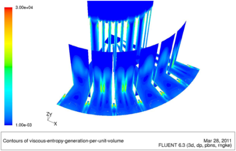In order to calculate these local rates, both the velocity and temperature field have to be completely resolved, and therefore a CFD solver, i.e., a distributed-parameter model, is needed. Once the entropy rates are known, thanks to the visualization tool of the solver, we can display the maps of ${\dot{s}}_T$ and ${\dot{s}}_V$, so that the designer is able to literally see where the entropy is produced at a higher rate and therefore where exergy is destroyed at a higher rate; it is possible to pinpoint the areas where we should focus our attention on.

2. The LED Spotlight

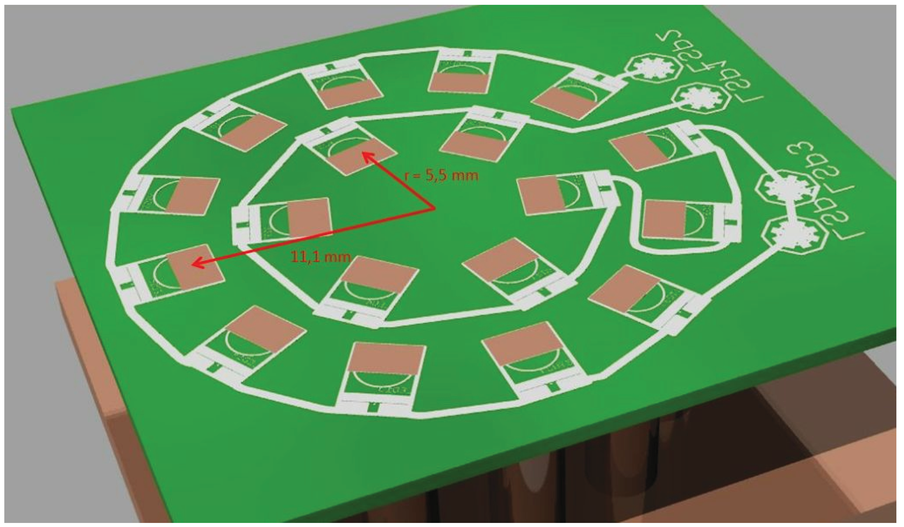
Eighteen diodes are printed on a fibreglass plate to form a LED spotlight whose layout and dimensions are shown in Figure 1 and Figure 2. Every diode dissipates 3 W and the maximum allowed temperature of the plate (and of the base of each diode) is 80 °C. In addition, the temperature difference between the diodes should not exceed 10 °C. In order to level out the temperatures of the diodes, a so called “thermal pad”, consisting of a 70 µm thick copper film, is placed under the plate.

Figure 1. The diode spotlight.

Figure 1. The diode spotlight.

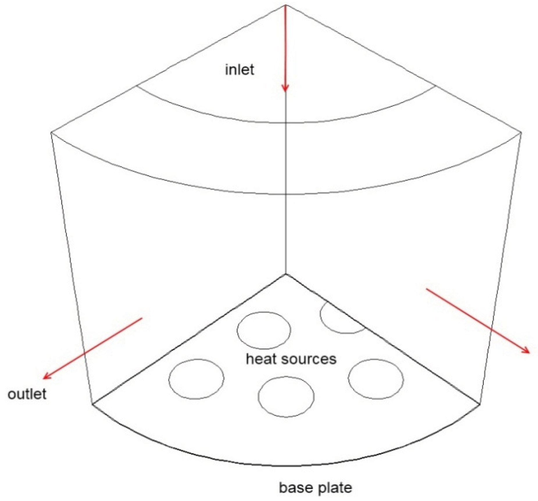
The cooling relies on the forced convection driven by a jet of air impinging on the thermal pad that lies on the bottom of the fibreglass plate shown in Figure 1. In order to assess the temperature field in the absence of heat transfer augmentation surfaces, the simple geometry S-1 is designed and simulated. Taking advantage of the symmetries of the geometry, only a 90° portion of the spotlight is modelled. This geometry consists of the copper plate only, cooled by the impinging air (see Figure 3). The inlet mass flow is determined assuming an increase of the air temperature of $\Delta T_{air}=5$:

$$\dot{m}=\frac{\dot{Q}}{c_{p,air}\cdot \Delta T_{air}}=\frac{3\cdot 18}{1006.43\cdot 5}=0.001731\cdot kg/s$$

(1)

At steady-state, the average temperature of the base is approximately 250 °C, which is unacceptable. Therefore, several complex geometries of aluminium fins for heat transfer augmentation are designed and simulated. A pseudo-optimization process is carried out via a successive series of design modifications based on a careful analysis of the local entropy generation maps. The design modifications concern mostly the fin spacing and dimensions.

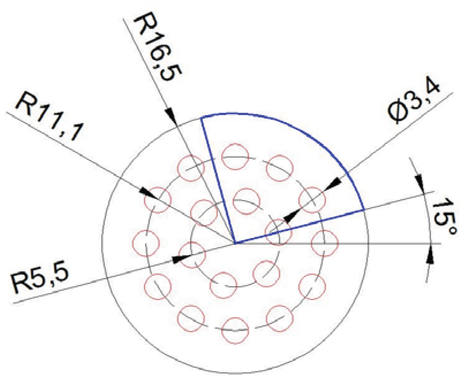
Figure 2. Planar view of the spotlight. The diodes (heat sources) are indicated by red circles. Only the blue sector is modelled in this study.

Figure 2. Planar view of the spotlight. The diodes (heat sources) are indicated by red circles. Only the blue sector is modelled in this study.

Figure 3. Geometry S-1.

Figure 3. Geometry S-1.

3. Alternative Geometries

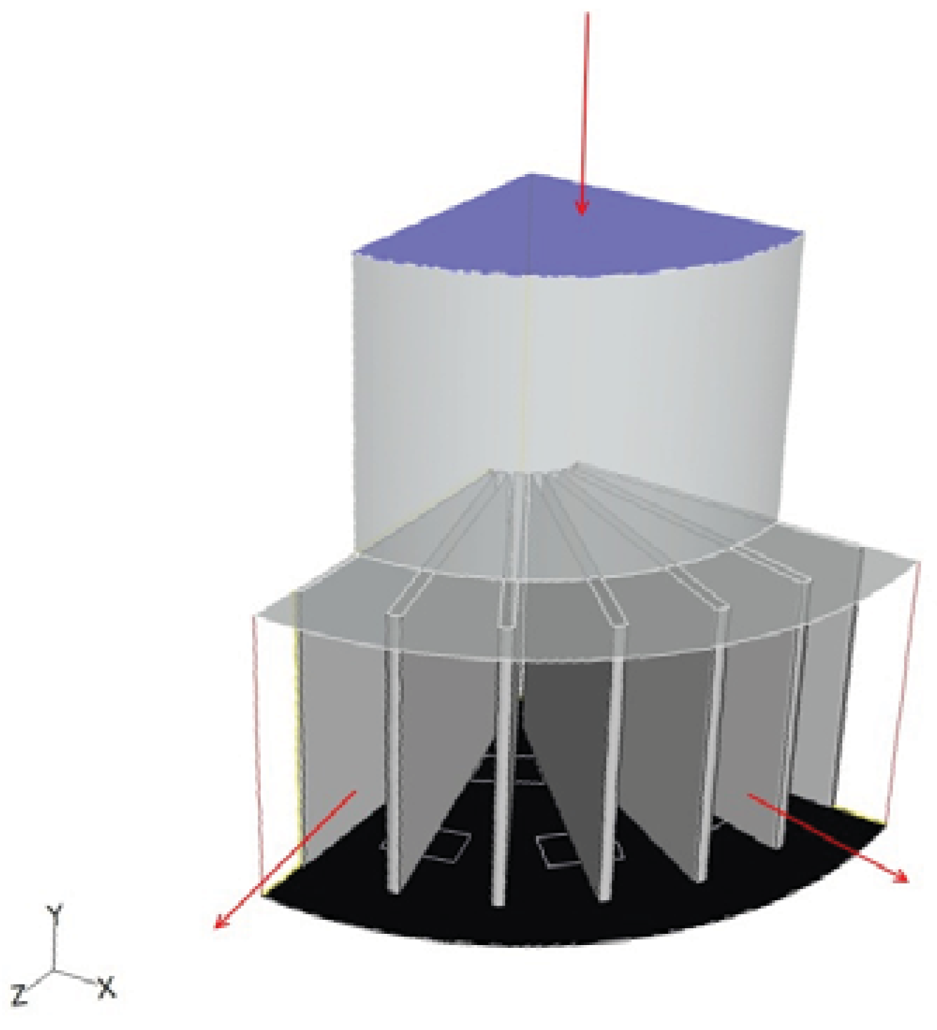
Geometry S-2 features periodically spaced in the radial direction aluminium plate-fins 0.75 mm thick, 12 mm high and 12 mm long. Since the external diodes are equally spaced at 30° and the internal ones at 60°, it is decided to place one fin every 15° for a total of 24 fins (six per quadrant), so that each diode is “covered” by one plate-fin. As shown in Figure 4, the domain has been slightly modified. In order to ensure structural stability of the fins (the fluid enters the domain with v_inlet ≈ 20 m/s) two physical walls have been added. The heat sources are modelled as rectangles for ease of mesh generation.

Figure 4. Geometry S-2.

Figure 4. Geometry S-2.

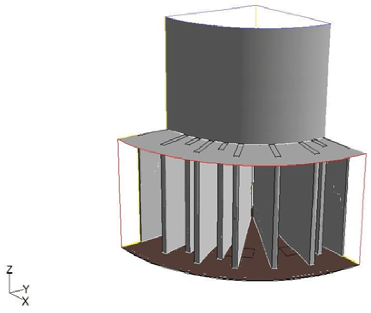
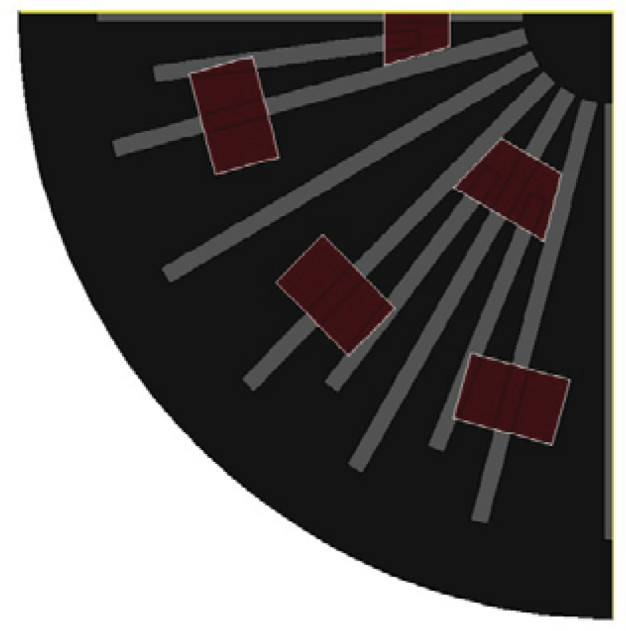
In order to further improve heat transfer and lower the average temperature of the diodes, geometry S-3 is designed and simulated (Figure 5). Geometry S-3 features 12 additional shorter fins placed where the diodes are denser and the heat flux is maximum (see Figure 6).

Figure 5. Geometry S-3.

Figure 5. Geometry S-3.

Figure 6. Bottom view of geometry S-3.

Figure 6. Bottom view of geometry S-3.

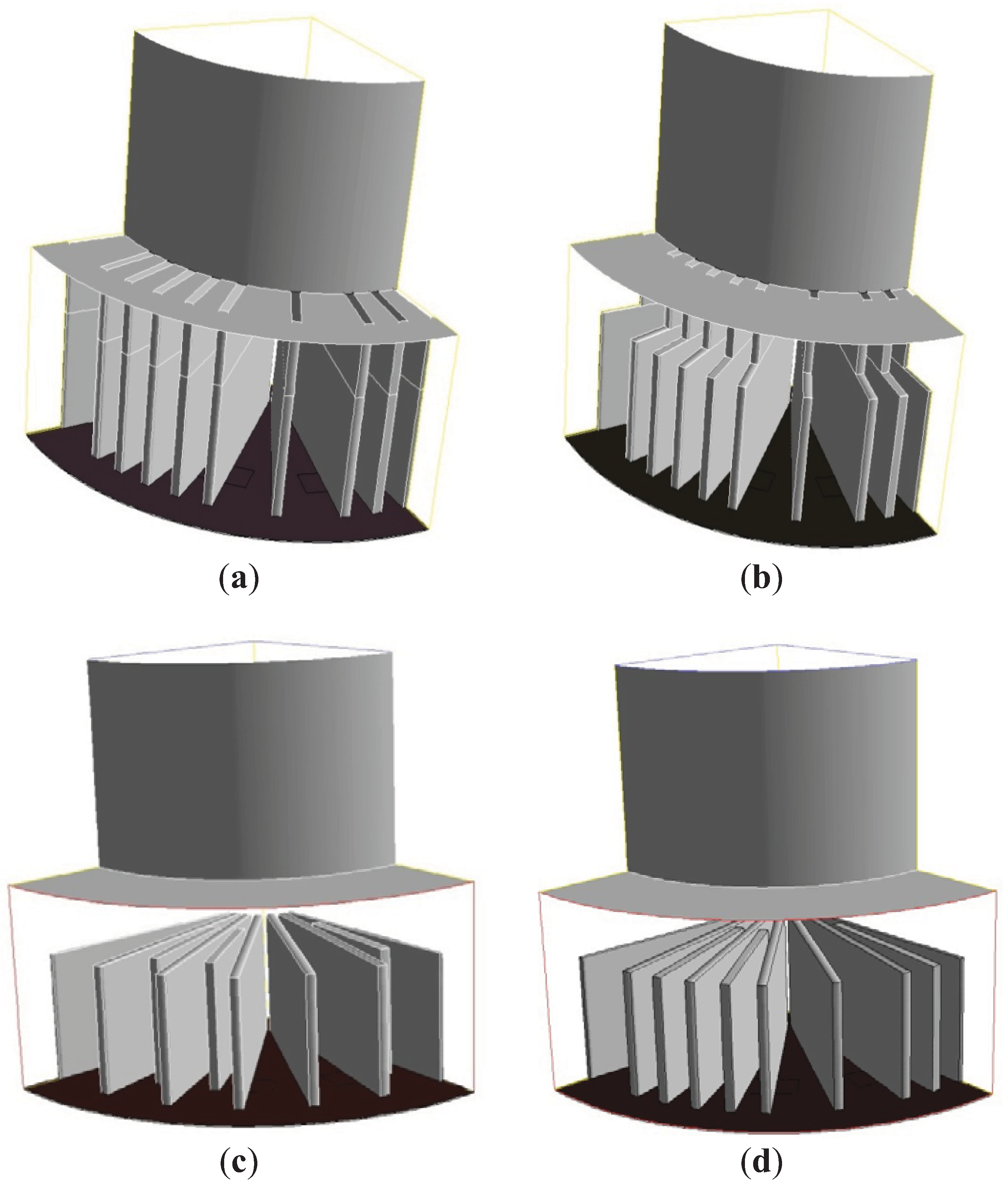
In geometry S-3, the interstitial fins are shorter than the others. To simplify the geometry from a technological point of view, and augment the heat transfer area, geometry S-3-1 was designed (Figure 7a). For reasons that will be clear later, geometry S-3-1 is simply obtained by cutting the top external corner of the fins at z = 7 mm and r = 8 mm (Figure 7b). A complete cut at z = 7 mm is done for the other two geometries, S-3-3 in Figure 7c, and S-3-4 in Figure 7d. Both feature fins 7 mm high, but the former has shorter interstitial fins.

Figure 7. (a) Geometry S-3-1. (b) Geometry S-3-2. (c) Geometry S-3-3. (d) Geometry S-3-4.

Figure 7. (a) Geometry S-3-1. (b) Geometry S-3-2. (c) Geometry S-3-3. (d) Geometry S-3-4.

3.1. Strategy for Probing the Solution Space and Description of the Heuristic Procedure

The entropy generation rate can be shown, for the case in study (i.e., in the absence of phase changes and chemical reactions), to consist of two parts [2]: one, called “viscous” (${\dot{s}}_V$), that depends on the physical viscosity, on the local temperature of the fluid and on the square of the local variation of the velocity (velocity gradient), and another, called “thermal” (${\dot{s}}_T$), that depends on the physical conductivity, on the square of the local temperature of the fluid and on the square of local temperature gradient:

$${\dot{s}}_{gen}={\dot{s}}_T+{\dot{s}}_V=\frac{k}{T^2}\left[{\left(\frac{\partial T}{\partial x}\right)}^2+{\left(\frac{\partial T}{\partial y}\right)}^2+{\left(\frac{\partial T}{\partial z}\right)}^2\right]+\frac{\varphi }{T}$$

(2)

where ϕ is the rate of viscous dissipation per unit volume. Note that the entropy generation rate expressed in (2) is per unit volume (W/(K m³)). The global entropy generation rate ${\dot{S}}_{gen}$ of the entire domain (W/K) is computed simply as the integral of the local rates over the entire volume V:

$${\dot{S}}_{gen}={\displaystyle \underset{V}{\int }{\dot{s}}_{gen}}dV={\displaystyle \underset{V}{\int }({\dot{s}}_T+{\dot{s}}_V)}dV={\dot{S}}_T+{\dot{S}}_V$$

(3)

As mentioned above, the approach adopted in this work consists in focusing the attention first on the local entropy generation rates ${\dot{s}}_T$, ${\dot{s}}_V$ and in considering the global one ${\dot{S}}_{gen}$ only after having carefully studied the implications of the local irreversible losses. In particular, the procedure for ‘optimising’ a design by means of an entropy generation analysis is the following:

• Define a starting geometry or a family of starting geometries.
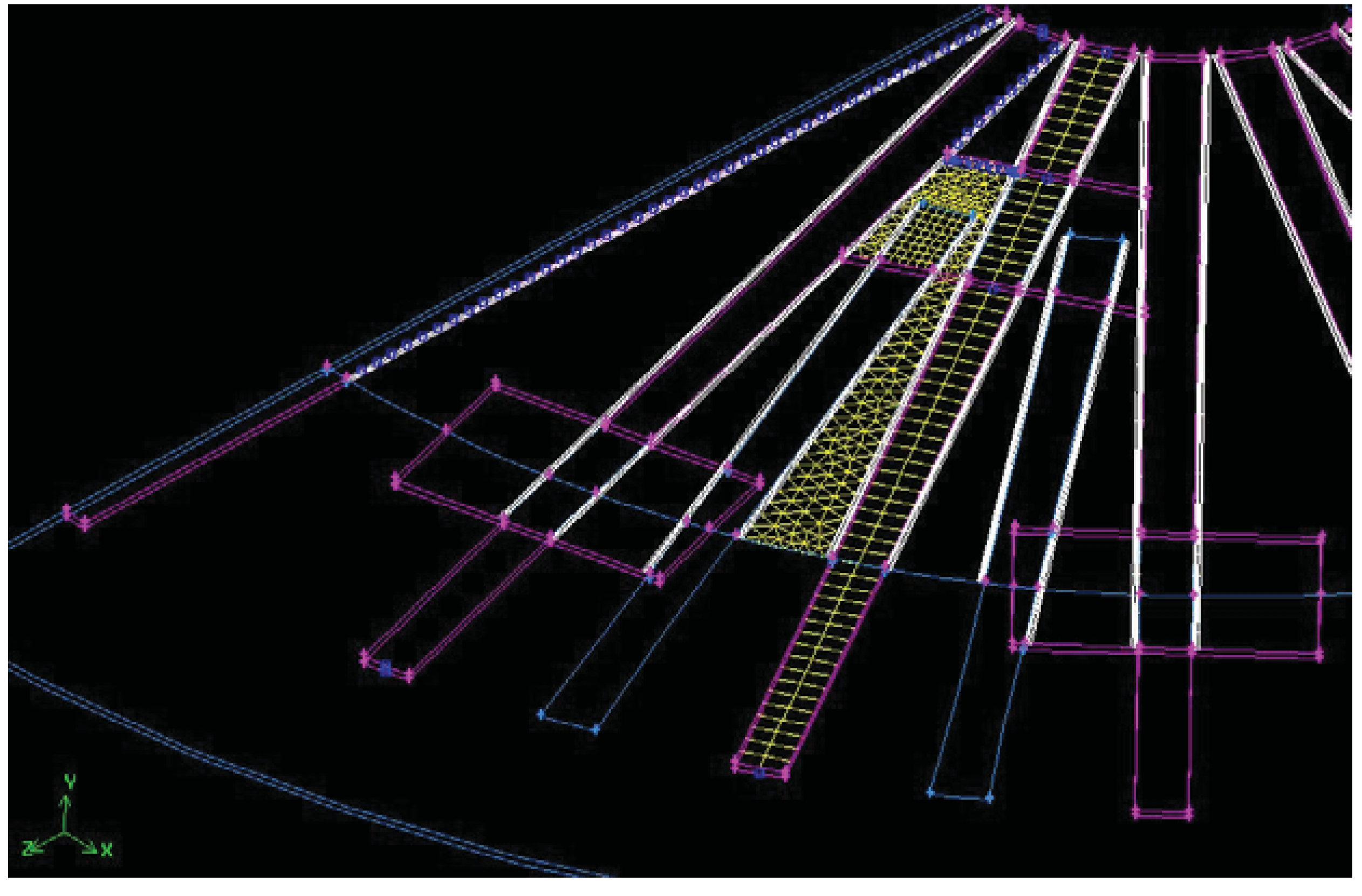
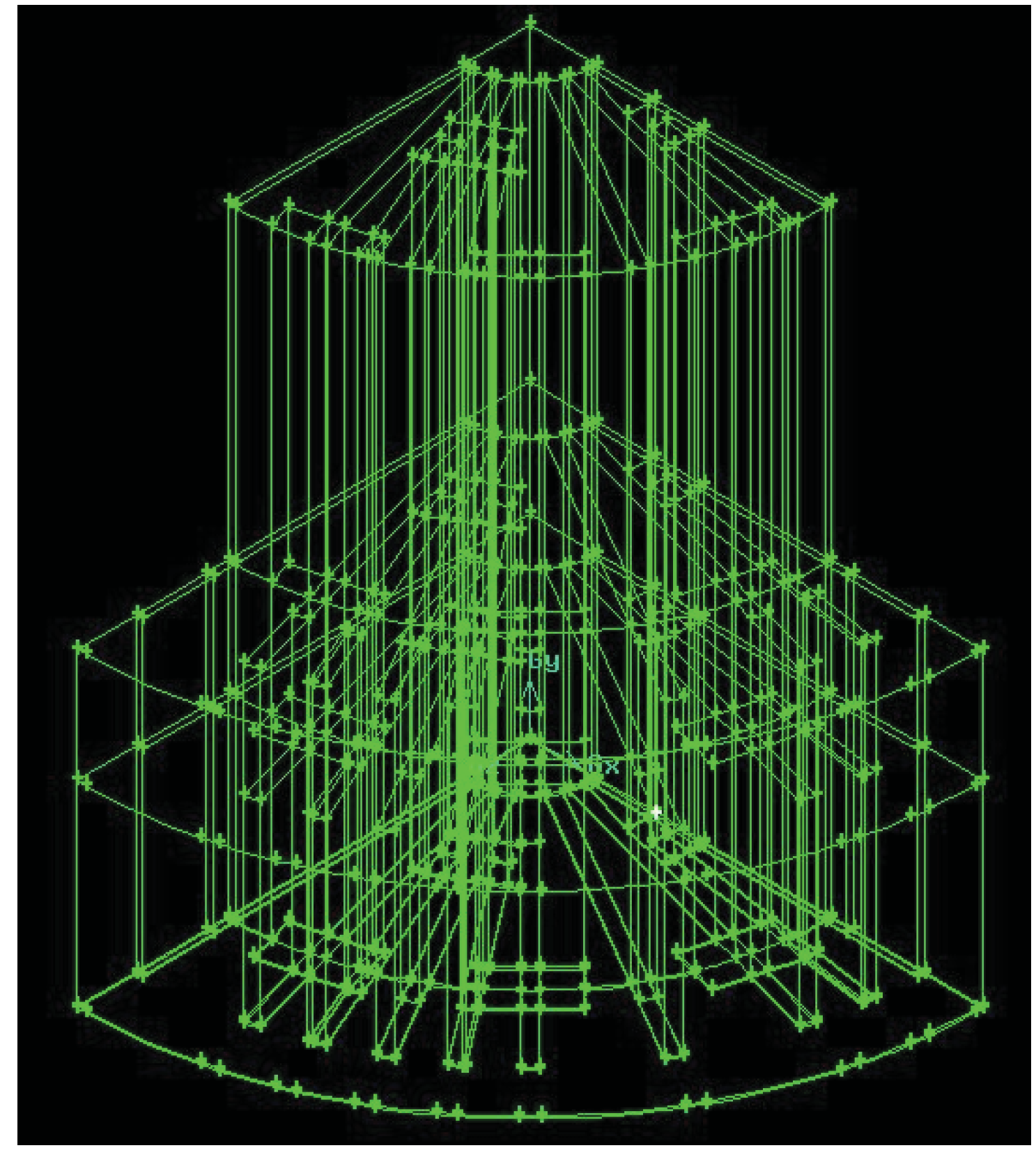
• Acquire the geometries and create the computational grid to be imported into the CFD solver.
• Compute the temperature and the velocity fields.
• Compute and display the maps of ${\dot{s}}_T$, ${\dot{s}}_V$.
• Integrate local values to obtain the global entropy generation rate ${\dot{S}}_{gen}$.
• Modify the design as suggested by a critical inspection of the local entropy maps.
• Repeat the computation, and iterate until a feasible and acceptable “minimum” of ${\dot{S}}_{gen}$ is obtained.

It is now clear that the process described above is not a proper optimization, but rather a heuristic design approach, essentially based on a thermodynamically sound trial-and-error procedure. Nevertheless, the amount of phenomenological information contained in the local entropy generation maps is so high that a convergence towards a better design is almost guaranteed [10].

4. The Numerical Simulations

4.1. Meshing

Neither IGES files nor other models were available for this problem. Therefore the different geometries are created from scratch directly in the mesh generator. As stated before, taking advantage of the symmetries of the geometry, only a 90° portion of the spotlight is modelled (as can be seen in Figure 2, the spotlight is circumferentially periodic with period of 60°; so, the modelled portion could have been further reduced to a sector of 60°; however, the choice of symmetrical boundary conditions rather than periodic ensures a faster convergence of the simulations, even if a larger volume needs to be meshed). The control volume of the spotlight includes the 70 µm thick copper film on which the surfaces representative of the heat sources are created, and a 22 mm height fluid volume which is obtained by sweeping the base plate surface in the direction perpendicular to the baseplate itself. The inlet surface and the base-plate have a radius of 11 mm and 16.5 mm, respectively. When other configurations are developed, the control volume is modified accordingly. As shown in Figure 8, when the fins (which have also been meshed) are introduced, the fluid volume is split into several other volumes. This technique allows for a better control of the mesh generation which becomes quite complicated for such complex geometries. The most critical zone is the base surface. As can be seen in Figure 9, this surface is divided into smaller sub-surfaces which represent the interface between the fins and the base plate and the projection of the heat sources (modelled as rectangles). Due to the complexity of the surface, a mixed mesh is used: the fluid zone is meshed with triangular elements, the fins with quadrilateral ones. Boundary layers are attached to the fins’ side as shown also in Figure 9. The adopted meshing scheme generates hexahedral or wedge cells only. Particular attention has been paid to the implementation of a high quality mesh with more than 95% of the elements having an Equisize Skew between 0 and 0.5. Before grid adaption the number of cells was ≈680,000.

Figure 8. Sub-volumes defined during the mesh generation process.

Figure 8. Sub-volumes defined during the mesh generation process.

Figure 9. Base-plate during the mesh generation.

Figure 9. Base-plate during the mesh generation.

4.2. Turbulent Model and Boundary Conditions

Since the flow is expected to be turbulent (Re_inlet ≈ 34,700) a turbulent model has to be chosen. The one adopted in this work is the RNG k − ε with enhanced wall functions. All simulations have been carried out at steady-state, therefore only the averaged terms in (2) are displayed and computed, but an effective viscosity µ_eff and an effective conductivity k_eff are employed. Being the flow fully turbulent, as required by the k – ε model, the viscosity and the thermal conductivity are evaluated via (4) and (5):

$${\mu }_{eff}=\mu +{\mu }_t$$

(4)

where µ is the molecular (laminar) viscosity and µ_t is the turbulent viscosity;

$$k_{eff}=k+k_t$$

(5)

where k is the molecular (laminar) thermal conductivity and kt is the turbulent thermal conductivity.

As discussed in [12,13], the k – ε model with standard wall function significantly underestimates the rate of entropy generation near the wall, but, to the knowledge of the authors, no studies have been carried out on the k – ε model with enhanced wall functions that FLUENT provides. In addition, it is intuitively clear that the turbulent model may misrepresent the local entropy generation: a detailed discussion of the problem is beyond the scope of this work and interested readers are referred to [13]. The boundary conditions are imposed as follows:

• Inlet: constant mass flow, equal to ¼ of the valued obtained in (1);
• Outlet: constant pressure, equal to atmospheric pressure;
• Diodes (heat sources): constant heat flux, 3 W per diode;
• Symmetry planes: zero gradients of all variables;
• Walls: impermeablility and no slip condition;
• External surface of the thermal pad: adiabatic impermeable wall.

4.3. Mesh Refinement

The next step involves a critical process: the grid sensitivity analysis. The goal of the mesh refinement is to demonstrate the mesh ability to capture the smallest (modellable) scales of the fluid dynamics phenomena involved in the simulation. An improved grid should be able to better describe the fluid behaviour and in order to determine the grid “quality” enhancement a cornerstone function field is needed for a performance comparison: the cornerstone function adopted in this work is the total entropy generation rate ${\dot{S}}_{gen}$, since in this case it is easily verified that the thermal and the viscous ones have the same order of magnitude. The adaption tool available in the solver permits to change the number of cells belonging to a grid, in both directions: coarsening and refinement. Excluding a priori any possibility of coarsening that will lead to a worse grid, the refinement can be operated with a criterion based on the gradient magnitude of the objective function. The gradient value is the difference of the values of the selected field function between two adjacent cells, therefore a large gradient indicates a potentially inaccurate numerical solution. The grid refinement should deliver a more efficient control volume, able to better evaluate the entropy generation rates. In fact, to increase the number of cells is tantamount to increase the numerical solver aptitude to capture the small-scale dissipative phenomena, which are reflected in the value of the entropy generation rates. In this perspective, a critical analysis on the magnitude distribution across the control volume of the gradient of the entropy generation rates has been performed. The next step has been the refinement of the grid, the “Grid Adaption”. The Refine Threshold has been set to approximately 5% of the values reported in the Max field (i.e., the maximum value of the adaption function). As suggested in [14], the adaption threshold value has not been changed during the successive mesh adaptions which were carried on until less than a 4% variation in the entropy rates was verified.

5. Results and Discussion

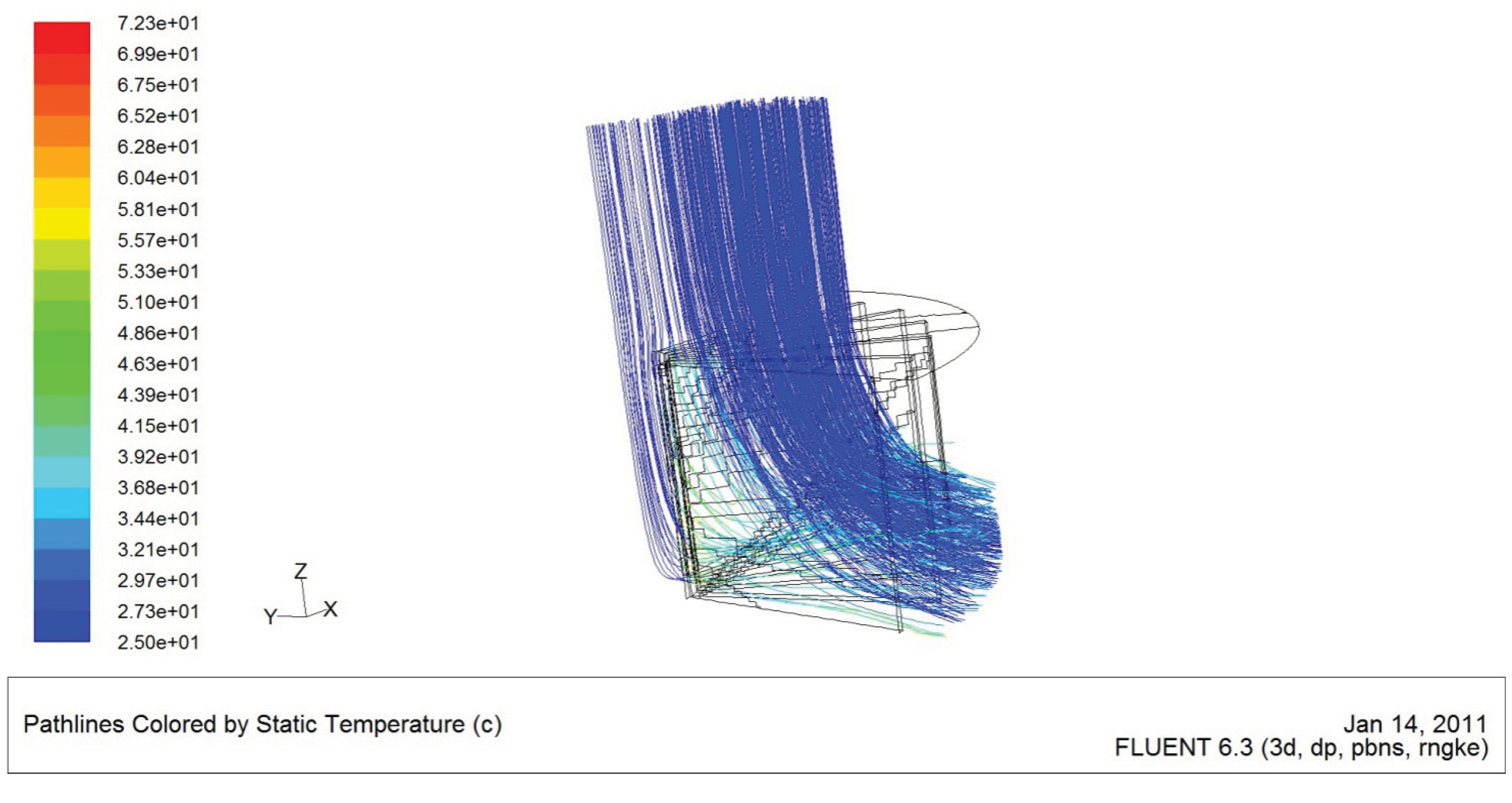
The simulation results of geometry S-2 are given in Table 1. The two sources of entropy are of the same order of magnitude. As shown in Figure 10, close to the outlet only the lower part of the fins is invested by the impinging jet.

Table 1. Simulation results for geometry all geometries. T_av,diodes is the average temperature of the diodes; ∆T_diodes is the maximum temperature difference between the diodes.

Geometry	Tav,diodes, °C	∆Tdiodes	${\dot{\mathit{S}}}_{\mathit{T}}$, W/K	${\dot{\mathit{S}}}_{\mathit{V}}$, W/K	${\dot{\mathit{S}}}_{\mathit{g}\mathit{e}\mathit{n}}$, W/K
S-2	67.5	3	5.19E-03	1.74E-03	6.92E-03
S-3	56.5	3	3.85E-03	2.89E-03	6.47E-03
S-3.1	55.4	4	3.71E-03	2.90E-03	6.62E-03
S-3.2	55.8	4	3.83E-03	2.83E-03	6.66E-03
S-3.3	70.0	4	5.38E-03	1.13E-03	6.51E-03
S-3.4	68.4	4	5.46E-03	1.16E-03	6.62E-03

Table 1. Simulation results for geometry all geometries. T_av,diodes is the average temperature of the diodes; ∆T_diodes is the maximum temperature difference between the diodes.

Geometry	Tav,diodes, °C	∆Tdiodes	${\dot{\mathit{S}}}_{\mathit{T}}$, W/K	${\dot{\mathit{S}}}_{\mathit{V}}$, W/K	${\dot{\mathit{S}}}_{\mathit{g}\mathit{e}\mathit{n}}$, W/K
S-2	67.5	3	5.19E-03	1.74E-03	6.92E-03
S-3	56.5	3	3.85E-03	2.89E-03	6.47E-03
S-3.1	55.4	4	3.71E-03	2.90E-03	6.62E-03
S-3.2	55.8	4	3.83E-03	2.83E-03	6.66E-03
S-3.3	70.0	4	5.38E-03	1.13E-03	6.51E-03
S-3.4	68.4	4	5.46E-03	1.16E-03	6.62E-03

Figure 10. Streamlines for the cooling arrangement S-2.

Figure 10. Streamlines for the cooling arrangement S-2.

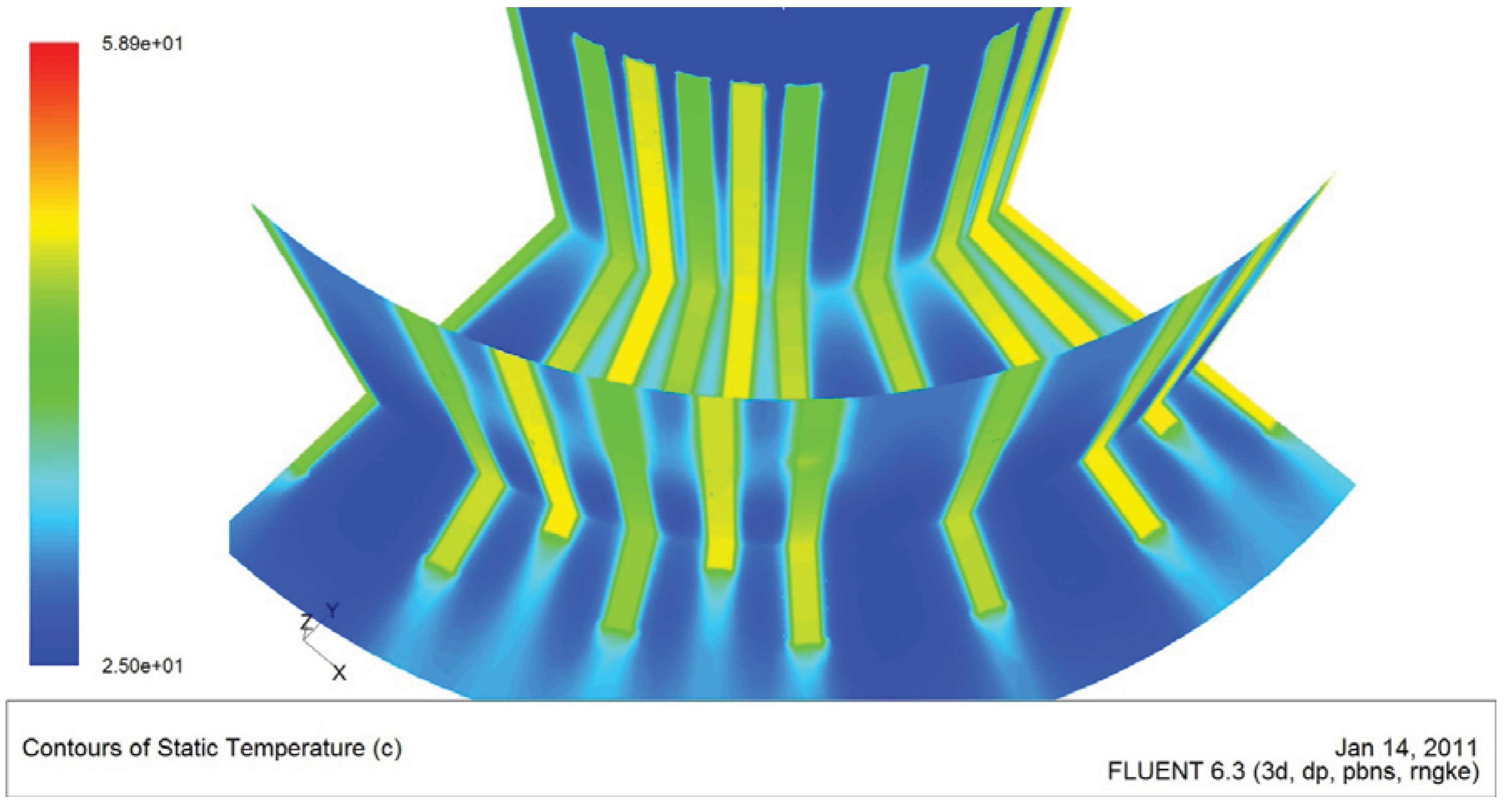
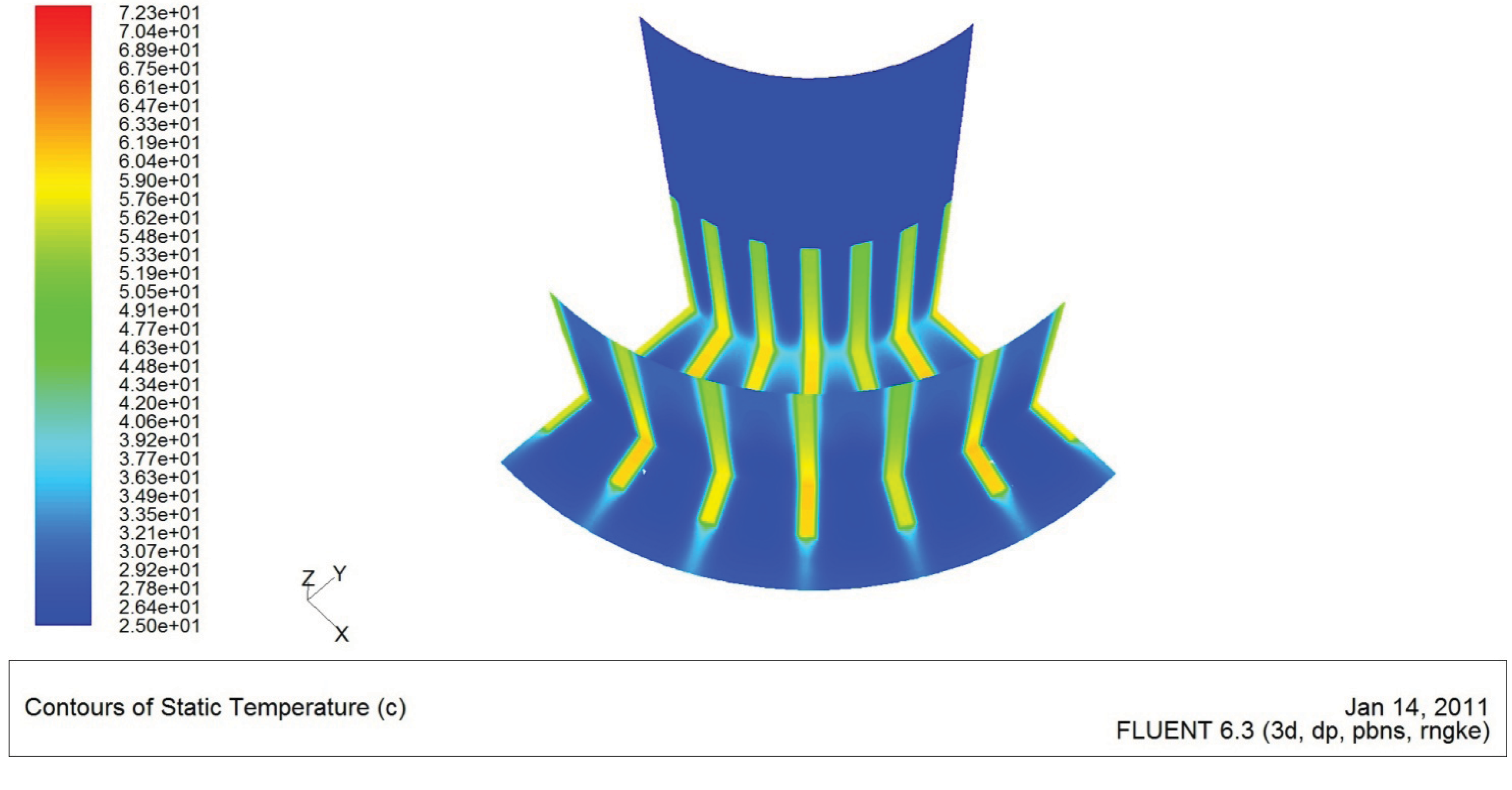
This causes a back flow in the upper and more external zone of the outlet where, however, the fluid has almost zero velocity: the fins are almost isolated being surrounded by a basically stagnant gas. Figure 11 shows the contours of temperatures in selected sections. The thermal boundary layers are clearly visible; they are very thin due the high velocities and very short characteristic length and they merge only very close to the baseplate due to its influence. In between the fins the flow is almost undisturbed.

Figure 11. Contours of temperature for geometry S-2 at z = 2 mm, r = 7 mm and r = 12.5 mm.

Figure 11. Contours of temperature for geometry S-2 at z = 2 mm, r = 7 mm and r = 12.5 mm.

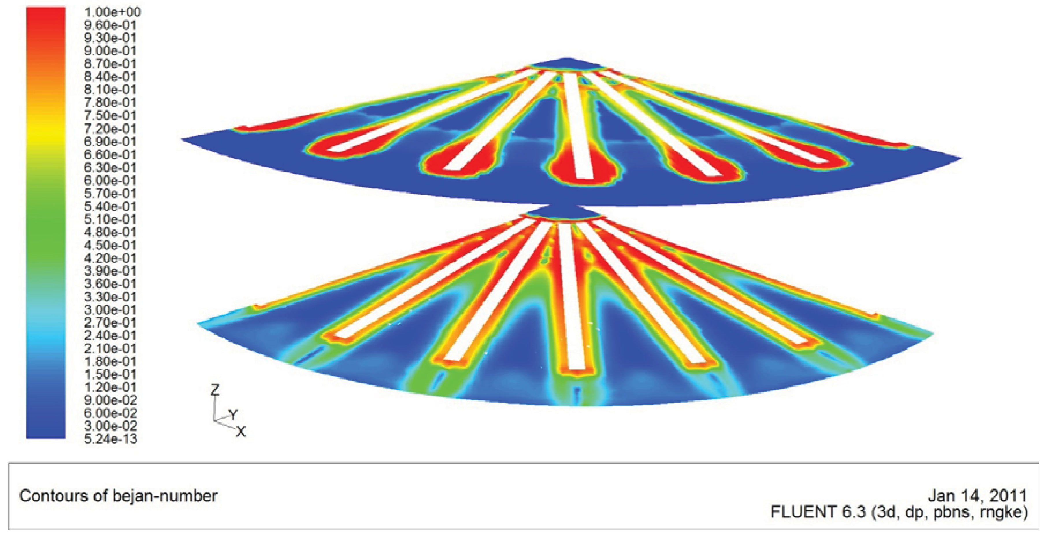
Figure 12 shows the distribution of the thermal entropy generation scaled by the total entropy generation rate (Be, Bejan number). Again, the influence of the boundary layer, both thermal and mechanical, is clearly visible. ${\dot{\mathit{s}}}_{\mathit{T}}$ has a stronger influence close to the baseplate and in the stagnation zone, where the velocities are lower. 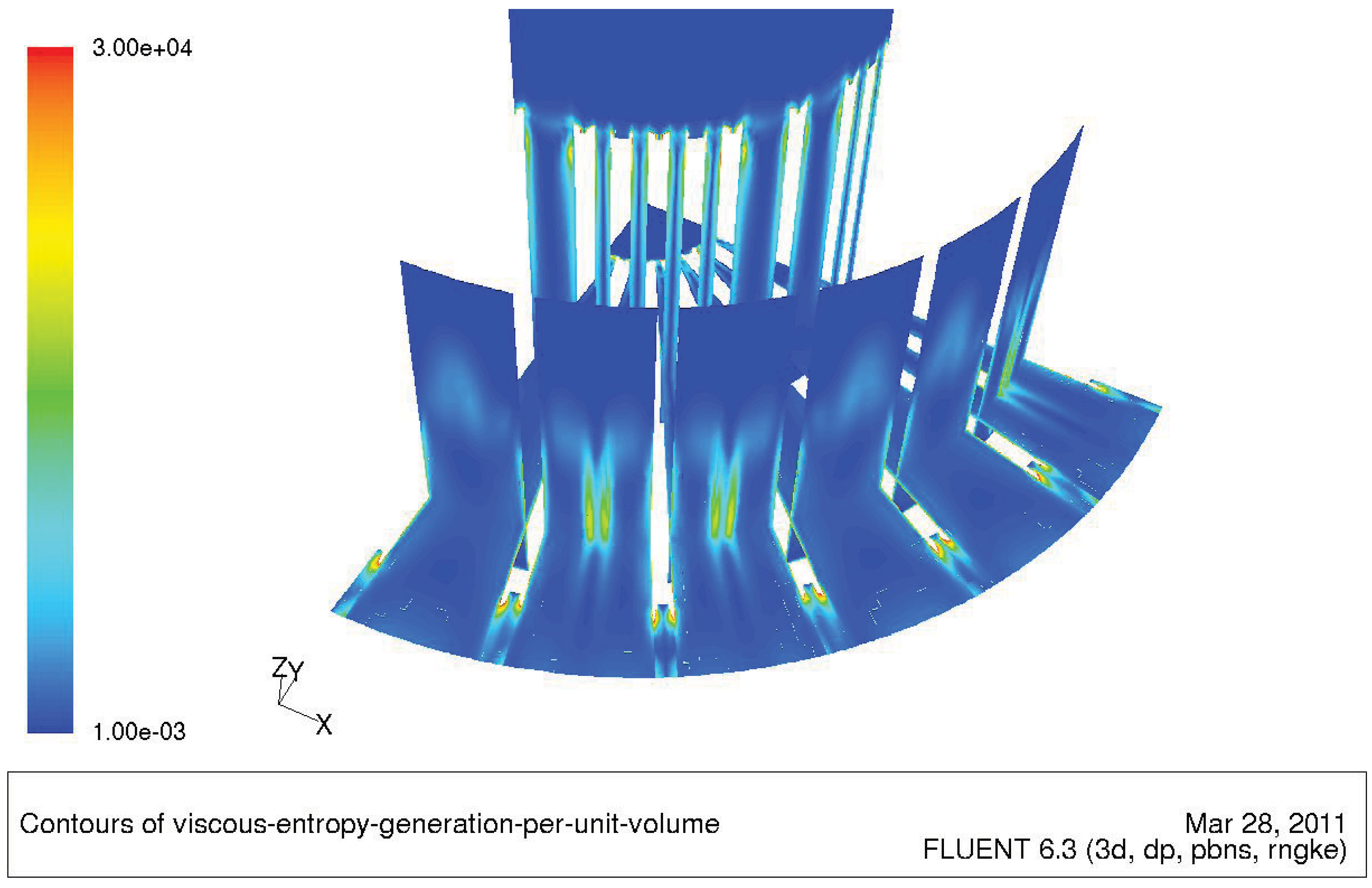In addition, almost only ${\dot{\mathit{s}}}_{\mathit{T}}$ is produced in the upper external zone of the fins where, as mentioned above, the fins are exchanging heat with an almost stagnant fluid. On the contrary, ${\dot{\mathit{s}}}_{\mathit{V}}$ is predominant in between the fins and in the wakes. A high ${\dot{\mathit{s}}}_{\mathit{V}}$ zone is present at the interface of the high velocity entering flow with the ambient (coming from the outlet) flow, as can be seen also in Figure 13.

Figure 12. Contours of the Bejan number Be for geometry S-2 at z = 2 mm and z = 8 mm.

Figure 12. Contours of the Bejan number Be for geometry S-2 at z = 2 mm and z = 8 mm.

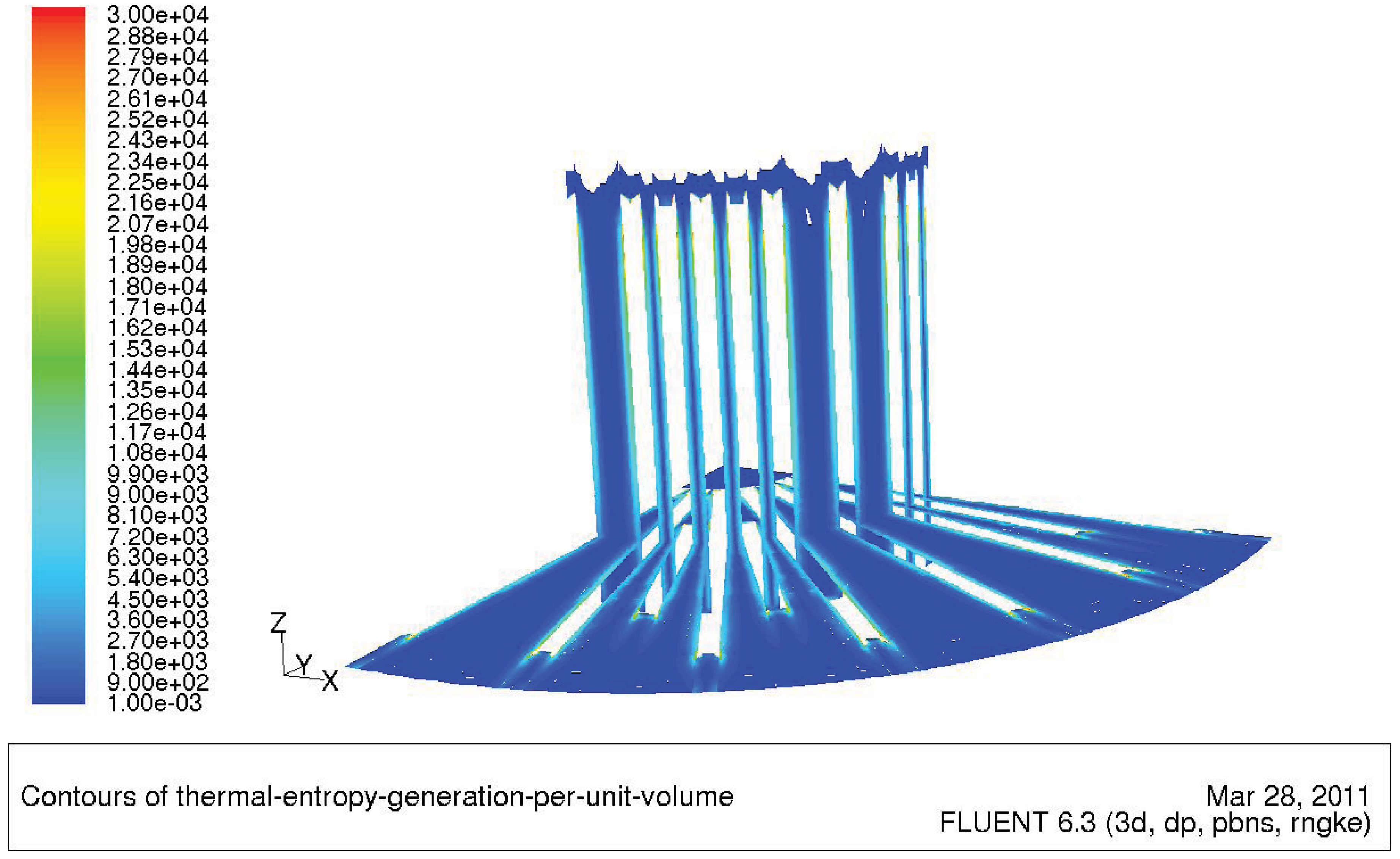
Figure 13. Contours of ${\dot{\mathit{s}}}_{\mathit{V}}$ for geometry S-2 at z = 2 mm, r = 7 mm and r = 12.5 mm.

Figure 13. Contours of ${\dot{\mathit{s}}}_{\mathit{V}}$ for geometry S-2 at z = 2 mm, r = 7 mm and r = 12.5 mm.

Figure 14. Contours of ${\dot{\mathit{s}}}_{\mathit{T}}$ for geometry S-2 at z = 2 mm and r = 7 mm.

Figure 14. Contours of ${\dot{\mathit{s}}}_{\mathit{T}}$ for geometry S-2 at z = 2 mm and r = 7 mm.

As stated before Geometry S-3 features 12 additional shorter fins placed where the diodes are more densely packed and the heat flux is maximum (see Figure 6). Even with the insertion of additional fins, the boundary layers merge only near the baseplate (Figure 15).

Figure 15. Contours of temperature for geometry S-3 at z = 2 mm, r = 7 mm and r = 12.5 mm.

Figure 15. Contours of temperature for geometry S-3 at z = 2 mm, r = 7 mm and r = 12.5 mm.

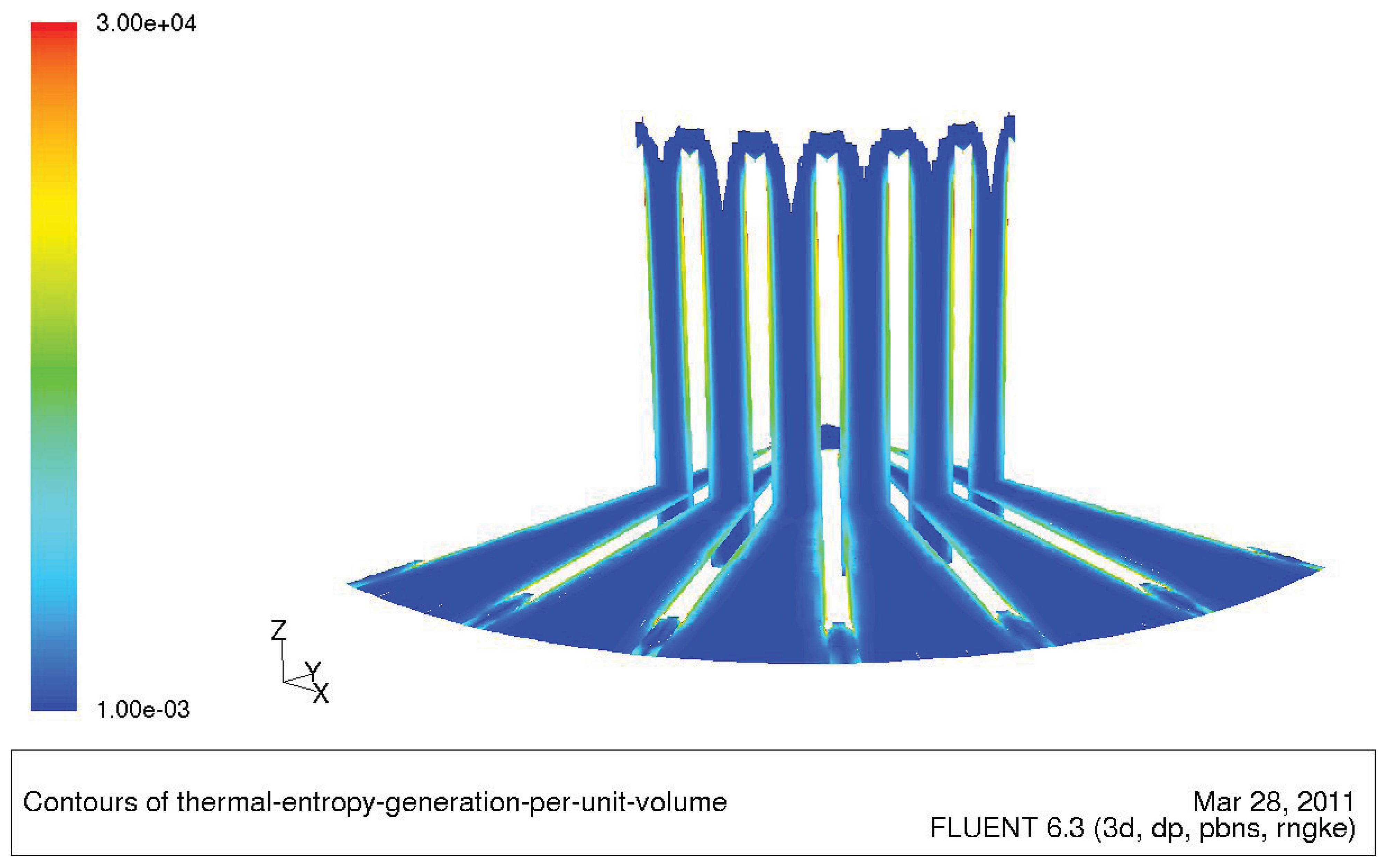
Nevertheless, since the boundary layers are close to each other, in these zones ${\dot{\mathit{s}}}_{\mathit{T}}$ reaches lower values than for geometry S-2 (see Figure 14 and Figure 16) and over the whole volume the thermal entropy generation rate drops of about 26% (Table 1).

Figure 16. Contours of ${\dot{\mathit{s}}}_{\mathit{T}}$ for geometry S-3 at z = 2 mm, r = 7 mm.

Figure 16. Contours of ${\dot{\mathit{s}}}_{\mathit{T}}$ for geometry S-3 at z = 2 mm, r = 7 mm.

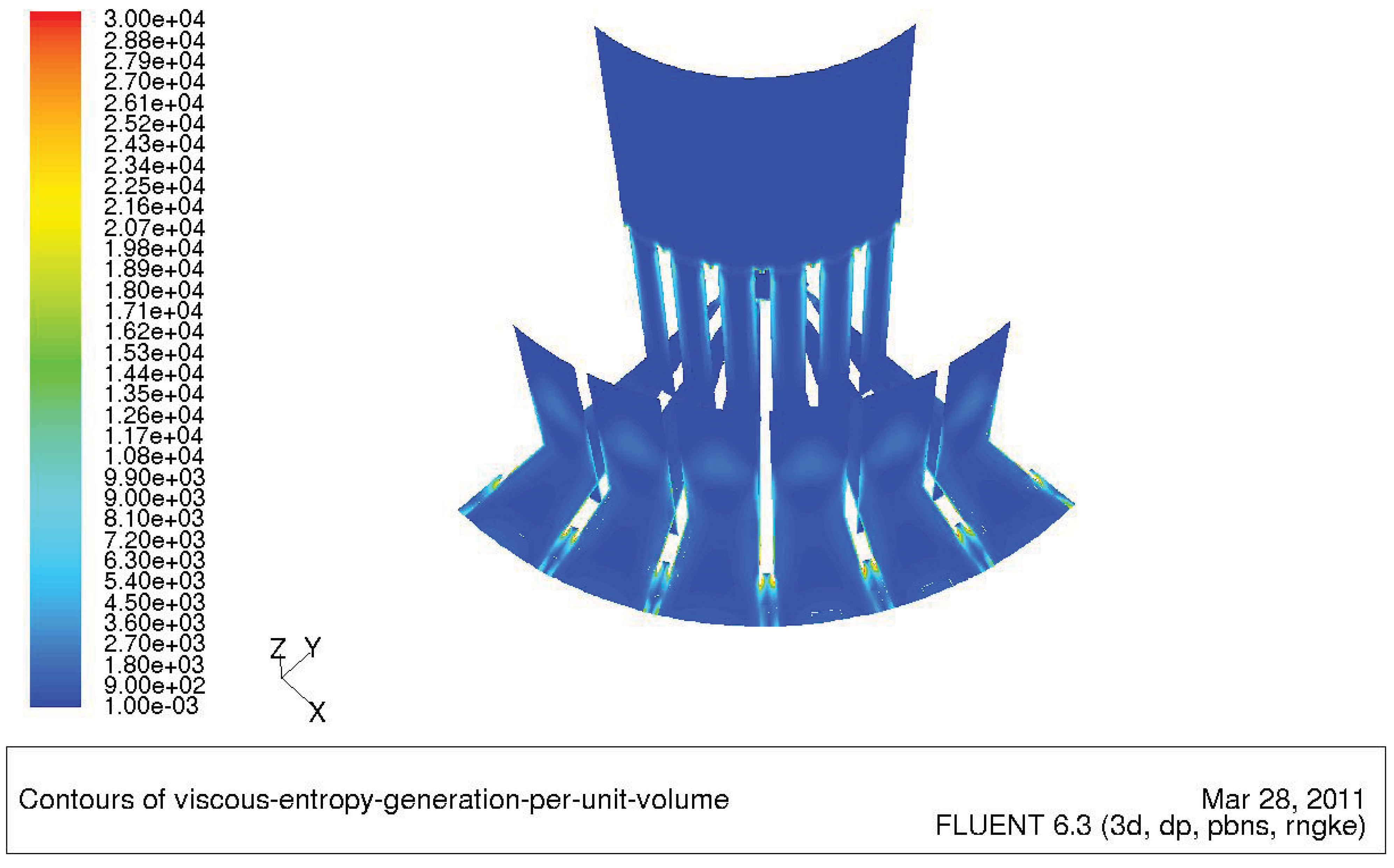
However, the presence of the added fins causes also an increase of about 67% in the viscous entropy generation. In fact, new vortices appear at the external end of the fins where the vorticity, ${\dot{\mathit{s}}}_{\mathit{V}}$ and the turbulent kinetic energy k all reach their peak values. The presence of the added fins, in fact, causes a local increment of the pressure whose effects propagates upstream; therefore, the mass flow is no longer evenly distributed between the channels bounded by the fins but attains lower values where the inter-fin spacing are lower. Higher velocities lead to high viscous dissipation in the larger channels (Figure 17).

Figure 17. Contours of ${\dot{\mathit{s}}}_{\mathit{v}}$ for geometry S-3 at z = 2 mm, r = 7 mm and r = 12.5 mm.

Figure 17. Contours of ${\dot{\mathit{s}}}_{\mathit{v}}$ for geometry S-3 at z = 2 mm, r = 7 mm and r = 12.5 mm.

In conclusion, ${\dot{S}}_{gen}$ is almost the same in both geometries, even though the relative contributions of the two portions ${\dot{\mathit{s}}}_{\mathit{T}}$ and ${\dot{\mathit{s}}}_{\mathit{v}}$ are completely different. In particular, the noticeable difference between the thermal entropy generation rate is reflected by the difference of the average temperatures of the diodes: T_av,diodes is 56.5 °C and 67.5 °C in geometry S-3 and S-2, respectively.

In geometry S-3, the interstitial fins have been designed shorter than the others. However, as can be seen in Figure 15, the thermal wake behind the shorter fins does not merge the thermal boundary layers of the longer fins due to the relatively cold and almost undisturbed stream coming from the inlet at high velocity; this stream quickly absorbs the wake. Therefore to simplify the geometry from a technological point of view, and augment the heat transfer area, geometry S-3-1 was designed (Figure 7a). Looking at Table 1, it can be seen that no appreciable differences are found in the entropy rates (less than 5% difference) while the T_av,diodes is one degree lower.

As for geometry S-2, the same behaviour in the upper and more external zone of the volume exists for S-3 and S-3-1. In these areas, the fins are almost isolated, are surrounded by a gas basically stagnant, and therefore are ineffective. For this reasons geometries S-3-2, S-3-3, and S-3.4 were designed. While S-3.2 has the lowest thermal entropy rate (and lower average temperature of the diodes), the other two produce a considerably smaller ${\dot{S}}_V$ but their lower heat transfer area leads to higher temperatures. 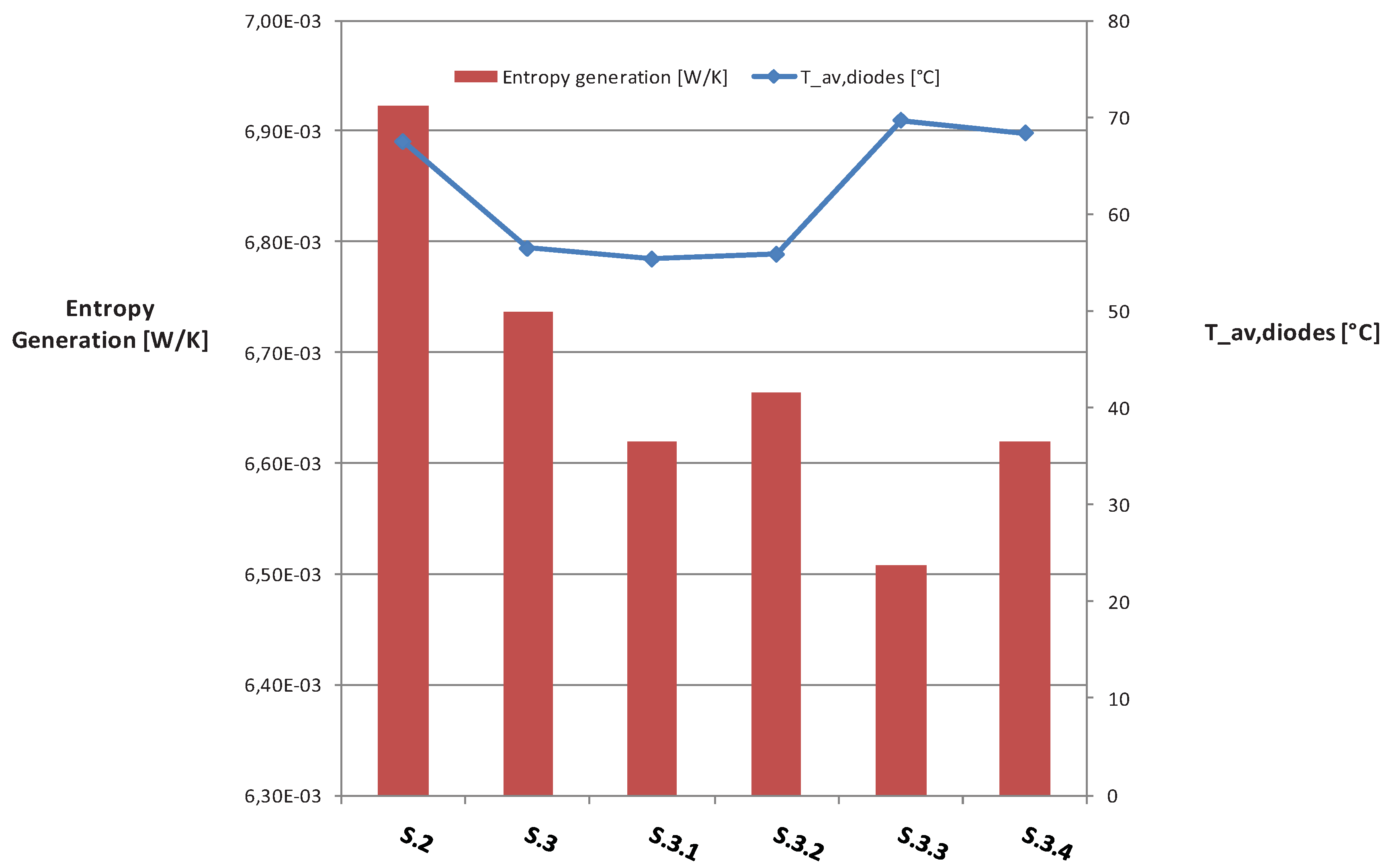As shown in Figure 18, the global production of entropy for all the S geometries is almost the same (the maximum difference is less than 6%), therefore from a thermodynamic perspective they perform equally. The discriminating factor is, though, the difference in their respective average temperatures. Since the characteristic velocities are comparable, the heat transfer coefficients are practically constant for all three configurations; therefore, the heat transfer is, with a good degree of approximation, directly proportional to the heat transfer area. In this perspective the best geometries are S-3, S-3-1 and S-3-2. It should be mentioned that the colour of the light shed by the diodes depends on their temperature, which for the purposes of this particular application should not exceed ≈80 °C. When one of the former geometries has been chosen, there are two ways to vary this temperature: to augment the voltage under which the diodes operate or to decrease the inlet air mass flow rate. The temperatures of the diodes in the geometries with less heat transfer area would be more sensible to the variations of the inlet mass flow.

Figure 18. Global entropy production rate ${\dot{S}}_{gen}$ and average temperature of the diodes T_av,diodes for all S geometries.

Figure 18. Global entropy production rate ${\dot{S}}_{gen}$ and average temperature of the diodes T_av,diodes for all S geometries.

5.1. Required Fan Power and Final Comparisons

The specific work per unit time that the fan has to deliver to the fluid can be calculated as:

$$P=\frac{\dot{m}\Delta p_{tot}}{\rho }$$

(6)

where:

$$\Delta p_{tot}={\left(p+\frac{\rho v^2}{2}\right)}_{outlet}-{\left(p+\frac{\rho v^2}{2}\right)}_{inlet}$$

(7)

The results for all the S geometries are given in Table 2. As expected, the geometries which features the highest heat transfer area are also the most power demanding ones.

Table 2. Required fan power for the indicated geometries.

Geometry	m, kg/s	ρ, kg/m3	∆ptot, Pa	P, W
S-2	0.010731	1.2	501	4.5
S-3	0.010731	1.2	814	7.3
S-3.1	0.010731	1.2	789	7.1
S-3.2	0.010731	1.2	786	7.0
S-3.3	0.010731	1.2	295	2.6
S-3.4	0.010731	1.2	297	2.7

Table 2. Required fan power for the indicated geometries.

Geometry	m, kg/s	ρ, kg/m3	∆ptot, Pa	P, W
S-2	0.010731	1.2	501	4.5
S-3	0.010731	1.2	814	7.3
S-3.1	0.010731	1.2	789	7.1
S-3.2	0.010731	1.2	786	7.0
S-3.3	0.010731	1.2	295	2.6
S-3.4	0.010731	1.2	297	2.7

A typical CPU dissipates around 35–50 W and the cooling usually relies on 90 × 90 × 70 mm aluminum plate-fin heat sinks, with a 80 mm fan on top. Such a fan usually produces 50 m³/h ≈ 0.017 kg/s, which means that air enters the heat sink with an average velocity of ≈3 m/s. As stated above, the spotlight has very small dimensions: therefore, even if the mass flow and the temperature field are comparable, the needed average inlet velocity is much higher, as it is the required fan power. However, radially placed fins provide higher heat transfer coefficients and employ less material even though their fabrication process is more complicated.

5.2. Conclusions

The thermodynamic fields, in all simulations, have been evaluated on a grid satisfactorily refined, using the total entropy generation rate as an objective function. In this way, a sufficiently large and reliable database of “experiments” has been obtained. The pseudo-optimization process in this work has proved to be an effective tool in the hands of a designer: in fact, a significant improvement of the thermodynamic performance has been obtained. The adopted procedure for “optimizing” a design by means of an entropy generation analysis is not an optimization proper, but rather a heuristic design approach, essentially based on a thermodynamically sound trial-and-error procedure. It results from the direct scanning of a finite (and in general quite small) solution set and is more similar to a (single or multiple parameter) sensitivity study. Nevertheless, the amount of phenomenological information contained in the local entropy generation maps is so high and detailed that a better design can always be defined. In this specific case, it was found that the best performance is attained when the fins are periodically spaced in the radial direction. In particular, all six geometries S-2, S-3, S-3-1, S-3-2, S-3-3 and S-3-4 can effectively cool the array of diodes while keeping the base-plate temperature well below 80 °C. Even though the global entropy production rate varies relatively very little between the configurations, big differences are found in the numerical values of the two sources of entropy ${\dot{S}}_T$ and ${\dot{S}}_V$. These differences are reflected in the average temperature of the diodes and in the required fan power: the lower ${\dot{S}}_T$, the lower T_av,diodes; the higher ${\dot{S}}_V$, the higher the required fan power.