On the Thermodynamics of Classical Micro-Canonical Systems

Abstract

We give two arguments why the thermodynamic entropy of non-extensive systems involves Rényi’s entropy function rather than that of Tsallis. The first argument is that the temperature of the configurational subsystem of a mono-atomic gas is equal to that of the kinetic subsystem. The second argument is that the instability of the pendulum, which occurs for energies close to the rotation threshold, is correctly reproduced.

1. Introduction

The recent interest in the micro-canonical ensemble [1,2,3,4,5,6,7,8,9,10,11,12,13] is driven by the awareness that this ensemble is the cornerstone of statistical mechanics. Phase transitions described in the canonical ensemble could be linked to topological singularities of the micro-canonical energy landscape [14,15,16,17,18,19,20]. On the other hand, the occurrence of thermodynamic instabilities in closed systems is not yet fully understood. In the canonical ensemble the situation is much clearer. Phase transitions are identified with the occurrence of analytical singularities in thermodynamic functions such as the free energy. These singularities can only occur in the thermodynamic limit. It is known [6,11,18] that such singularities appear frequently in the thermodynamic functions of isolated systems, even without considering the thermodynamic limit. This leads to the conclusion that micro-canonical phase transitions cannot be characterised in this way.

The present paper focuses on the configurational probability distribution of a mono-atomic gas with N interacting particles within a non-quantum-mechanical micro-canonical description. Recently [21], it was proved that this distribution belongs to the q-exponential family [22,23,24], with $q=1-2/(3N-2)$. In the thermodynamic limit $N\to \infty$ it converges to the Boltzmann-Gibbs distribution, which corresponds with the $q=1$ case. This observation of q-exponentiality is relevant for the discussion of phase transitions because it implies thermodynamic stability. Indeed, within a large class of entropy functions the Tsallis entropy function is unique (up to a multiplicative and an additive constant) in being maximized by the members of the q-exponential family. The corresponding free energy is then minimized. The minimality of the free energy is a sign of thermodynamic stability and of absence of phase transitions.

It was argued in [21] that for the calculation of thermodynamic quantities Rényi’s entropy function is more appropriate than that of Tsallis. The Rényi entropy function is a monotone function of that of Tsallis. Both entropy functions are maximized by the same probability distributions. Hence, Rényi’s entropy function is also maximized by the members of the q-exponential family. However, the corresponding free energy is not necessarily minimized, while this is necessarily so [22] in the Tsallis case. As a consequence, a description in terms of Rényi’s entropy function leaves room for thermodynamic instabilities, while these are not possible when starting from the Tsallis function.

Note that here and throughout the paper we mean by thermodynamic instability a negative heat capacity or, equivalently, a convex region of entropy S as a function of energy U. Strictly spoken, the perfectly isolated microcanonical system is not unstable. However, if two identical systems with negative heat capacity and slightly different energy are in contact through a small leak in the thermal insulation, then energy will flow from the system low in energy to that with more energy. In this way the energy difference will increase until the separation into a low energy phase and a high energy phase is completed. Phase separations of this type do occur in closed systems and can rightfully be called a sign of thermodynamic instability.

Most concepts of thermodynamics can get a very precise definition within the canonical ensemble of statistical mechanics. But clearly, large parts of thermodynamics are also valid for isolated systems. However, up to now the concepts of thermodynamics have not been validated within the context of the micro-canonical ensemble. 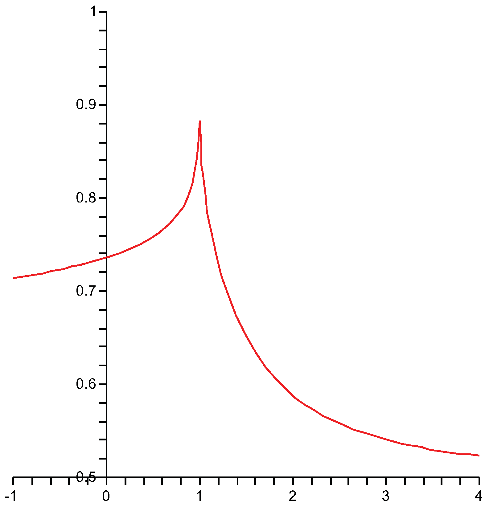We contribute to this goal by studying a simple example in which it is intuitively clear that two distinct thermodynamic phases [25] are present. The pendulum serves this goal because it has two distinct types of orbits: librational motion at low energy and rotational motion at high energy. The density of states $\omega \left(U\right)$ can be calculated analytically (see for instance [26]). It has a logarithmic singularity at the energy $U_c$, which is the minimum value needed to allow rotational motion—see the Figure 1.

The thermodynamic quantity central to the micro-canonical ensemble is the entropy $S\left(U\right)$ as a function of the total energy U. Therefore, we start with it in the next Section, which discusses the configurational probability distribution and its properties. Section 3 compares the use of Rényi’s entropy functional with the use of that of Tsallis. Section 4 deals with the example of the pendulum. The final Section draws some conclusions. The short Appendix clarifies certain calculations.

Figure 1. Density of states of the pendulum in reduced units. Shown is the function ${\omega }_0\left(u\right)$ as defined by (36).

Figure 1. Density of states of the pendulum in reduced units. Shown is the function ${\omega }_0\left(u\right)$ as defined by (36).

2. The Configurational Subsystem

The entropy $S\left(U\right)$, which is most often used for a gas of point particles in the classical micro-canonical ensemble, is

$$\begin{array}{c}\hfill S\left(U\right)=k_{B}ln\omega \left(U\right)\end{array}$$

(1)

where $\omega \left(U\right)$ is the N-particle density of states. It is given by

$$\begin{array}{c}\hfill \omega \left(U\right)=c_N{\int }_{{\mathbb{R}}^{3N}}\mathrm{d}{\mathbf{p}}_1\cdots \mathrm{d}{\mathbf{p}}_N{\int }_{{\mathbb{R}}^{3N}}\mathrm{d}{\mathbf{q}}_1\cdots \mathrm{d}{\mathbf{q}}_N\delta (U-H(\mathbf{q},\mathbf{p}))\end{array}$$

(2)

Here, ${\mathbf{q}}_j$ is the position of the j-th particle and ${\mathbf{p}}_j$ is the conjugated momentum, $H(\mathbf{q},\mathbf{p})$ is the Hamiltonian. The constant $c_N$ equals $1/N!h^{3N}$. The constant h has the same dimension as Planck’s constant. It is inserted for dimensional reasons. This definition goes back to Boltzmann’s idea of equal probability of the micro-canonical states and the corresponding well-known formula $S=k_{B}lnW$, where W is the number of micro-canonical states.

The shortcomings of Boltzmann’s entropy have been noticed long ago. A slightly different definition of entropy is [27,28,29,30,31,32] (see also in [33] the reference to the work of A. Schlüter)

$$\begin{array}{c}\hfill S\left(U\right)=k_{B}ln\Omega \left(U\right)\end{array}$$

(3)

where $\Omega \left(U\right)$ is the integral of $\omega \left(U\right)$ and is given by

$$\begin{array}{c}\hfill \Omega \left(U\right)=c_N{\int }_{{\mathbb{R}}^{3N}}\mathrm{d}{\mathbf{p}}_1\cdots \mathrm{d}{\mathbf{p}}_N{\int }_{{\mathbb{R}}^{3N}}\mathrm{d}{\mathbf{q}}_1\cdots \mathrm{d}{\mathbf{q}}_N\Theta (U-H(\mathbf{q},\mathbf{p}))\end{array}$$

(4)

Here, $\Theta \left(x\right)$ is Heaviside’s function. An immediate advantage of Equation (3) is that the resulting expression for the temperature T, defined by the thermodynamic formula

$$\begin{array}{c}\hfill \frac{1}{T}=\frac{\mathrm{d}S}{\mathrm{d}U}\end{array}$$

(5)

coincides with the experimentally used notion of temperature. Indeed, there follows immediately

$$\begin{array}{c}\hfill k_{B}T=\frac{\Omega \left(U\right)}{\omega \left(U\right)}\end{array}$$

(6)

It is well-known that for classical mono-atomic gases the r.h.s. of Equation (6) coincides with twice the average kinetic energy per degree of freedom. Hence, the choice of (3) as the thermodynamic entropy has the advantage that the equipartition theorem, assigning $k_{B}T/2$ to each degree of freedom, does hold for the kinetic energy also in the micro-canonical ensemble.

The micro-canonical ensemble is described by the singular probability density function

$$\begin{array}{c}\hfill f_U(\mathbf{q},\mathbf{p})=\frac{1}{\omega \left(U\right)}\delta (U-H(\mathbf{q},\mathbf{p}))\end{array}$$

(7)

where $\delta \left(x\right)$ is Dirac’s delta function. The normalization is so that

$$\begin{array}{c}\hfill 1=c_N{\int }_{{\mathbb{R}}^{3N}}\mathrm{d}{\mathbf{p}}_1\cdots \mathrm{d}{\mathbf{p}}_N{\int }_{{\mathbb{R}}^{3N}}\mathrm{d}{\mathbf{q}}_1\cdots \mathrm{d}{\mathbf{q}}_N{f}_U(\mathbf{q},\mathbf{p})\end{array}$$

(8)

For simplicity, we take only one conserved quantity into account, namely the total energy. Its value is fixed to U.

In the simplest case the Hamiltonian is of the form

$$\begin{array}{c}\hfill H(\mathbf{q},\mathbf{p})=\frac{1}{2m}\sum _{j=1}^N{\left|{\mathbf{p}}_j\right|}^2+\mathcal{V}\left(\mathbf{q}\right)\end{array}$$

(9)

where $\mathcal{V}\left(\mathbf{q}\right)$ is the potential energy due to interaction among the particles and between the particles and the walls of the system. It is then possible to integrate out the momenta. This leads to the configurational probability distribution, which is given by

$$\begin{array}{ccc}\hfill f_U^{\mathrm{conf}}\left(\mathbf{q}\right)& =& {\left(\frac{a}{h}\right)}^{3N}{\int }_{{\mathbb{R}}^{3N}}\mathrm{d}{\mathbf{p}}_1\cdots \mathrm{d}{\mathbf{p}}_N{f}_U(\mathbf{q},\mathbf{p})\hfill \end{array}$$

(10)

The normalization is so that

$$\begin{array}{ccc}\hfill 1& =& \frac{1}{N!a^{3N}}{\int }_{{\mathbb{R}}^{3N}}\mathrm{d}{\mathbf{q}}_1\cdots \mathrm{d}{\mathbf{q}}_N{f}_U^{\mathrm{conf}}\left(\mathbf{q}\right)\hfill \end{array}$$

(11)

The constant a has been introduced for dimensional reasons [34]. In the limit of an infinitely large system, this configurational system is described by a Boltzmann-Gibbs distribution. However, here we are interested in small systems where an exact evaluation of (10) is necessary. A straightforward calculation yields

$$\begin{array}{ccc}\hfill f_U^{\mathrm{conf}}\left(\mathbf{q}\right)& =& \frac{{[U-\mathcal{V}\left(\mathbf{q}\right)]}_{+}^{3N/2-1}}{{ϵ}^{3N/2}\omega \left(U\right)\Gamma (3N/2)}\hfill \end{array}$$

(12)

with $ϵ=h^2/2\pi m{a}^2$. This result has been known since long.

It was shown in [21] that the configurational probability distribution $f_U^{\mathrm{conf}}\left(\mathbf{q}\right)$ belongs to the q-exponential family, with $q=1-\frac{2}{3N-2}$. This implies [22,23,24] that it maximizes the expression

$$\begin{array}{c}\hfill I\left(f\right)-\theta U^{\mathrm{conf}}\left(f\right)\end{array}$$

(13)

for some value of θ, where

$$\begin{array}{c}\hfill I\left(f\right)=-\frac{1}{1-q}\frac{1}{N!a^{3N}}{\int }_{{\mathbb{R}}^{3N}}\mathrm{d}{\mathbf{q}}_1\cdots \mathrm{d}{\mathbf{q}}_{N}f\left(\mathbf{q}\right)\left[{\left(f\left(\mathbf{q}\right)\right)}^{1-q}-1\right]\end{array}$$

(14)

with

$$\begin{array}{c}\hfill U^{\mathrm{conf}}\left(f\right)=\frac{1}{N!a^{3N}}{\int }_{{\mathbb{R}}^{3N}}\mathrm{d}{\mathbf{q}}_1\cdots \mathrm{d}{\mathbf{q}}_{N}f\left(\mathbf{q}\right)\mathcal{V}\left(\mathbf{q}\right)\end{array}$$

(15)

Maximizing Equation (13) has been called the variational principle by the mathematical physics community of the 1980s. This property is stronger than the maximum entropy principle and corresponds with the principle of minimal free energy.

Note that $I\left(f\right)$ is the Tsallis entropy function [35,36] up to one modification (replacement of the parameter q by $2-q$) [37]. The parameter θ turns out to be given by

$$\begin{array}{c}\hfill \theta =\frac{2-q}{1-q}\frac{1}{{ϵ}^{2-q}{[\Gamma (3N/2)\omega \left(U\right)]}^{1-q}}\end{array}$$

(16)

The maximisation of Equation (13) is equivalent to the minimisation of the free energy (using $I\left(f\right)$ as the entropy function appearing in the definition of the free energy). Replacing the Boltzmann-Gibbs-Shannon (BGS) entropy function by $I\left(f\right)$ is necessary—the configurational probability distribution $f_U^{\mathrm{conf}}\left(\mathbf{q}\right)$ does not maximize the BGS entropy function as a consequence of finite size effects.

3. Rényi’s Entropy Function

It is tempting to identify the parameter θ of the previous Section with the inverse temperature $\beta =1/k_{\mathrm{B}}T$ and to interpret (13) as the maximisation of the entropy function $I\left(f\right)$ under the constraint that the average energy $U^{\mathrm{conf}}\left(f\right)$ equals the given value $U^{\mathrm{conf}}$. However, in [21] an example was given showing that this identification of θ with β cannot be correct in general. It was noted that replacing the Tsallis entropy function by that of Rényi gives a more satisfactory result. This argument is now repeated in a more general setting.

In the present context, Rényi’s entropy function of order α is defined by

$$\begin{array}{c}\hfill I^{\alpha }\left(f\right)=\frac{1}{1-\alpha }ln\left[\frac{1}{N!a^{3N}}{\int }_{{\mathbb{R}}^{3N}}\mathrm{d}{\mathbf{q}}_1\cdots \mathrm{d}{\mathbf{q}}_{N}f{\left(\mathbf{q}\right)}^{\alpha }\right]\end{array}$$

(17)

Let $\alpha =2-q$. Then (17) is linked to (14) by

$$\begin{array}{c}\hfill I^{\alpha }\left(f\right)=\xi \left(I\left(f\right)\right)\end{array}$$

(18)

with

$$\begin{array}{c}\hfill \xi \left(u\right)=\frac{1}{q-1}ln[1+(q-1)u]\end{array}$$

(19)

Note that

$$\begin{array}{c}\hfill \frac{\mathrm{d}\xi }{\mathrm{d}u}=\frac{1}{1+(q-1)u}\end{array}$$

(20)

This derivative is strictly positive on the domain of definition of $\xi \left(u\right)$. Hence, $\xi \left(u\right)$ is a monotonically increasing function. Therefore, the density $f\left(\mathbf{q}\right)$ is a maximizer of $I\left(f\right)$ if and only if it maximizes $I^{\alpha }\left(f\right)$. This means that from the point of view of the maximum entropy principle it does not make any difference whether one uses the Rényi entropy function or that of Tsallis. However, for the variational principle discussed in the previous Section, and for the definition of the temperature T via the thermodynamic formula (5) the function $\xi \left(u\right)$ makes a difference. In the example of the pendulum, discussed further on, the variational principle is not satisfied when using Rényi’s entropy function, while it is satisfied when using $I\left(f\right)$. Also, the derivation which follows below shows that, when Rényi’s entropy function is used, the temperature of the configurational subsystem equals the temperature T of the kinetic subsystem.

Let us now calculate the value of Rényi’s entropy function for the configurational probability distribution (10). One has

$$\begin{array}{c}\hfill I^{\alpha }\left(f_U^{\mathrm{conf}}\right)=\frac{1}{q-1}ln\left[\frac{1}{N!a^{3N}}{\int }_{{\mathbb{R}}^{3N}}\mathrm{d}{\mathbf{q}}_1\cdots \mathrm{d}{\mathbf{q}}_N{\left(f_U^{\mathrm{conf}}\left(\mathbf{q}\right)\right)}^{2-q}\right]\end{array}$$

(21)

Use now that (see (12))

$$\begin{array}{ccc}\hfill {\left(f_U^{\mathrm{conf}}\left(\mathbf{q}\right)\right)}^{1-q}& =& \frac{U-\mathcal{V}\left(\mathbf{q}\right)}{ϵ{[\Gamma (3N/2)ϵ\omega \left(U\right)]}^{1-q}}\hfill \end{array}$$

(22)

Then (21) simplifies to

$$\begin{array}{ccc}\hfill I^{\alpha }\left(f_U^{\mathrm{conf}}\right)& =& ln\Gamma \left(\frac{3N}{2}\right)ϵ\omega \left(U\right)-\left(\frac{3N}{2}-1\right)ln\frac{U^{\mathrm{kin}}}{ϵ}\hfill \end{array}$$

(23)

The claim is now that (23), when multiplied with $k_{\mathrm{B}}$, is the thermodynamic entropy $S^{\mathrm{conf}}\left(U\right)$ of the configurational subsystem. Note that $ϵ=h^2/2\pi m{a}^2$ is an arbitrary unit of energy. Note also that, using Stirling’s approximation and $U^{\mathrm{kin}}=3N\Omega \left(U\right)/2\omega \left(U\right)$, (23) simplifies to

$$\begin{array}{ccc}\hfill \frac{1}{k_{\mathrm{B}}}{S}^{\mathrm{conf}}\left(U\right)& \simeq & lnϵ\omega \left(U\right)-\left(\frac{3N}{2}-1\right)ln\frac{\Omega \left(U\right)}{ϵ\omega \left(U\right)}\hfill \end{array}$$

$$\begin{array}{ccc}& & +\left(\frac{3N}{2}-1\right)ln\left(\frac{3N}{2}-1\right)-\frac{3N}{2}+\frac{1}{2}ln3\pi N\hfill \end{array}$$

(24)

To support our claim, let us calculate its prediction for the temperature of the configurational subsystem. One finds

$$\begin{array}{ccc}\hfill \frac{1}{T^{\mathrm{conf}}}& \equiv & \frac{\mathrm{d}{S}^{\mathrm{conf}}}{\mathrm{d}{U}^{\mathrm{conf}}}=k_{\mathrm{B}}\left[\frac{{\omega }^{\prime }}{\omega }-\left(\frac{3N}{2}-1\right)\frac{1}{U^{\mathrm{kin}}}\right]\frac{\mathrm{d}U}{\mathrm{d}{U}^{\mathrm{conf}}}+k_{\mathrm{B}}\left(\frac{3N}{2}-1\right)\frac{1}{U^{\mathrm{kin}}}\hfill \end{array}$$

(25)

Using (see (26) of [21])

$$\begin{array}{c}\hfill \frac{\mathrm{d}{U}^{\mathrm{conf}}}{\mathrm{d}U}=1-\frac{3N}{2}+\frac{{\omega }^{\prime }}{\omega }{U}^{\mathrm{kin}}\end{array}$$

(26)

this becomes

$$\begin{array}{c}\hfill \frac{1}{T^{\mathrm{conf}}}=k_{\mathrm{B}}\frac{3N}{2U^{\mathrm{kin}}}=k_{\mathrm{B}}\frac{\omega }{\Omega }=\frac{1}{T}\end{array}$$

(27)

This shows that the configurational temperature, calculated starting from Rényi’s entropy function, coincides with the temperature T defined by means of the modified Boltzmann entropy (3) and with the temperature of the kinetic subsystem.

Finally, let us define a configurational heat capacity by

$$\begin{array}{c}\hfill C^{\mathrm{conf}}=\frac{\mathrm{d}{U}^{\mathrm{conf}}}{\mathrm{d}T}=T\frac{\mathrm{d}{S}^{\mathrm{conf}}}{\mathrm{d}T}\end{array}$$

(28)

Then one has in a trivial way

$$\begin{array}{c}\hfill C=\frac{\mathrm{d}U}{\mathrm{d}T}=\frac{\mathrm{d}}{\mathrm{d}T}\left[\frac{3}{2}N{k}_{\mathrm{B}}T+U^{\mathrm{conf}}\right]=\frac{3}{2}N{k}_{\mathrm{B}}+C^{\mathrm{conf}}\end{array}$$

(29)

Let us summarize the results obtained so far. The system under consideration is an interacting gas studied in the classical micro-canonical ensemble. The system is decomposed into two subsystems, the kinetic one and the configurational one. Each of them serves as the heat bath of the other. Both of them are in thermal equilibrium at the same temperature T, which is the temperature obtained in the standard way by taking the derivative of the micro-canonical entropy (3)—see (5). The temperature of the kinetic subsystem follows from the equipartition law. The temperature of the configurational subsystem is obtained by taking the derivative of Rényi’s entropy w.r.t. the configurational energy. The alpha parameter is given by $\alpha =2-q=3N/(3N-2)$.

Let us verify that the expression (23) makes sense even for an ideal gas. In this case the density of states is

$$\begin{array}{c}\hfill \omega \left(U\right)=\frac{c_N}{\Gamma (3N/2)}{V}^N{\left(2\pi m\right)}^{3N/2}{U}^{3N/2-1}\end{array}$$

(30)

Evaluation of (23) with $U^{\mathrm{kin}}=U$ then gives

$$\begin{array}{c}\hfill S^{\mathrm{conf}}=k_{\mathrm{B}}Nln\frac{V}{N{a}^3}+k_{\mathrm{B}}ln\frac{N^N}{N!}\simeq k_{\mathrm{B}}Nln\frac{eV}{N{a}^3}\end{array}$$

(31)

The configurational entropy of an ideal gas does not depend on the total energy or on the mass of the particles, as expected. The total entropy is

$$\begin{array}{ccc}\hfill S& =& k_{\mathrm{B}}ln\Omega \left(U\right)\hfill \end{array}$$

$$\begin{array}{ccc}& =& k_{\mathrm{B}}NlnV+\frac{3}{2}N{k}_{\mathrm{B}}ln2\pi mU+k_{\mathrm{B}}ln{c}_N-k_{\mathrm{B}}ln\Gamma (3N/2+1)\hfill \end{array}$$

(32)

Using Stirling’s approximation, (32) simplifies to

$$\begin{array}{c}\hfill S\simeq k_{\mathrm{B}}N\left(ln\frac{eV}{N{a}^3}+\frac{3}{2}ln2\pi \frac{U}{Nϵ}+constant\right)\end{array}$$

(33)

This expression coincides with the Sackur-Tetrode equation [38] for an appropriate choice of the constant term. The first term of (33) is the configurational entropy contribution (31), the second term is the kinetic energy contribution.

4. The pendulum

Let us now consider the example of the pendulum. The Hamiltonian reads

$$\begin{array}{c}\hfill H=\frac{1}{2I}{p}^2-{\kappa }^{2}Icos\left(\varphi \right)\end{array}$$

(34)

For low energy $-{\kappa }^{2}I<U<{\kappa }^{2}I$ the motion is oscillatory. At large energy $U>{\kappa }^{2}I$ it rotates in one of the two possible directions. The density of states $\omega \left(U\right)$ can be written as

$$\begin{array}{ccc}\hfill \omega \left(U\right)& =& \frac{\mathrm{d}}{\mathrm{d}U}\frac{2\sqrt{2I}}{h}\int \mathrm{d}\varphi \sqrt{U+I{\kappa }^{2}cos\varphi }\hfill \end{array}$$

$$\begin{array}{ccc}& =& \frac{4\pi \sqrt{2}}{h\kappa }{\omega }_0(U/{\kappa }^{2}I)\hfill \end{array}$$

(35)

with ${\omega }_0\left(u\right)$ given by

$$\begin{array}{ccc}\hfill {\omega }_0\left(u\right)& =& \frac{1}{2\pi }{\int }_0^1\mathrm{d}x\frac{1}{\sqrt{x}}\frac{1}{\sqrt{1-x}}\frac{1}{\sqrt{1-u+(1+u)x}}if-1<u<1,\hfill \end{array}$$

$$\begin{array}{ccc}\hfill {\omega }_0\left(u\right)& =& \frac{1}{2\pi }{\int }_{-1}^1\mathrm{d}x\frac{1}{\sqrt{1-x^2}}\frac{1}{\sqrt{x+u}}if1<u.\hfill \end{array}$$

(36)

See the Figure 1. Note that the integrals appearing in (36) are complete elliptic integrals of the first kind. For simplicity we choose now units in which ${\kappa }^{2}I=1$ holds. We also fix $h=4/\kappa$.

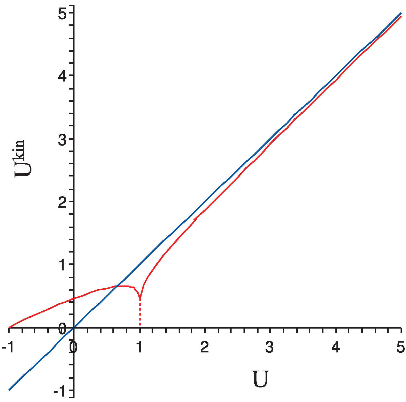
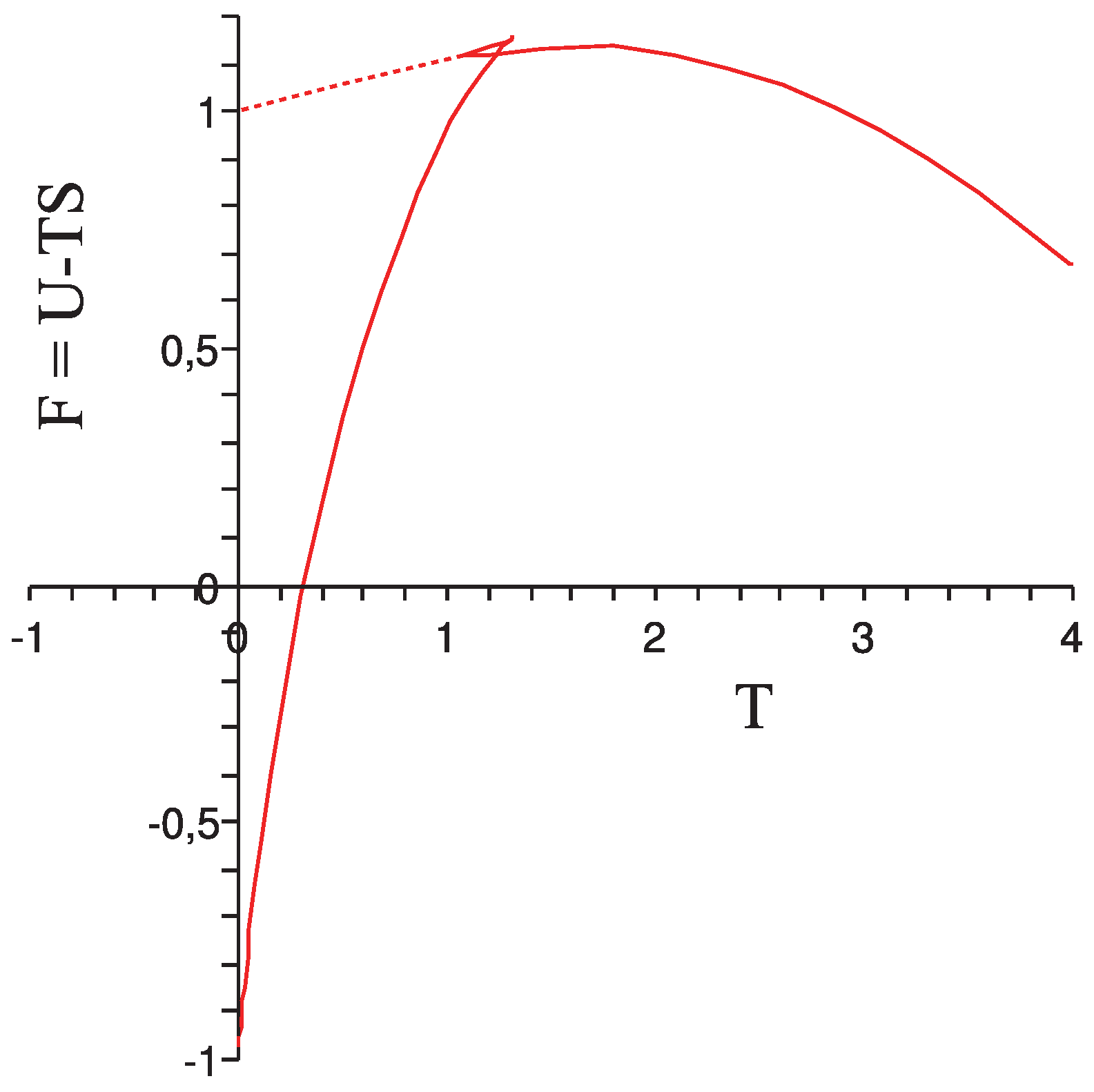
Using the analytic expressions (36), and the expression (6), it is straightforward to make a plot of the kinetic energy $U^{\mathrm{kin}}$ as a function of the energy U. See the Figure 2. Note that it is not a strictly increasing function. Due to the divergence of ${\omega }_0\left(u\right)$ at $u=1$ the temperature T has to vanish at both $u=-1$ and $u=+1$. Hence it has a maximum in between. This has consequences for the free energy F, which is the Legendre transform of $U\left(S\right)$. The well-known formula

$$\begin{array}{c}\hfill F\left(T\right)=U-TS\end{array}$$

(37)

is only valid if the entropy is a concave function of the energy. The result $F\left(T\right)$ is then a concave function. But if we substitute $U\left(T\right)$ in the r.h.s. of (37) then we obtain a multi-valued function. See the Figure 3.

Figure 2. Kinetic energy $U^{\mathrm{kin}}$ as a function of energy U.

Figure 2. Kinetic energy $U^{\mathrm{kin}}$ as a function of energy U.

Figure 3. Free energy of the pendulum.

Figure 3. Free energy of the pendulum.

When a fast rotating pendulum slows down due to friction then its energy decreases slowly. The average kinetic energy, which is the temperature $\frac{1}{2}{k}_{\mathrm{B}}T$, tends to zero when the threshold $U_c$ is approached. In Figure 3, the continuous curve is followed. The pendulum goes from a stable into a metastable rotational state. then it switches to an unstable librating state, characterised by a negative heat capacity. Finally it goes through the metastable and stable librational states. The first order phase transition [25] cannot take place because in a nearly closed system the pendulum cannot get rid of the latent heat. Neither can it stay at the phase transition point because a coexistence of the two phases cannot be realised.

For the example of the pendulum the number of degrees of freedom $3N$ in the expression for the non-extensivity parameter q has to be replaced by 1, so that $q=3$ results. This is an anomalous value because $0<q<1$ has been assumed in the main part of the paper. See the Appendix for a discussion of the modifications needed to treat this situation.

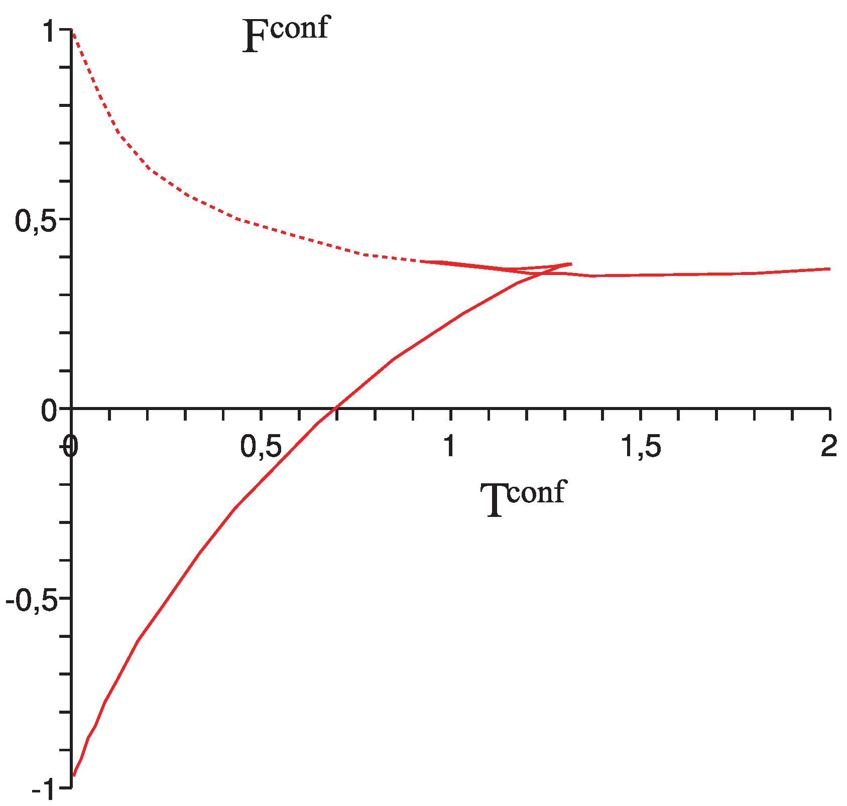
It remains true that the configurational probability distribution $f_U^{\mathrm{conf}}\left(\varphi \right)$ maximizes the Rényi entropy with $\alpha =2-q=-1$ within the set of all probability distributions having the same average potential energy $U^{\mathrm{conf}}$. Next, using

$$\begin{array}{ccc}\hfill \frac{1}{T^{\mathrm{conf}}}& \equiv & \frac{\mathrm{d}{S}^{\mathrm{conf}}}{\mathrm{d}{U}^{\mathrm{conf}}}\hfill \end{array}$$

(38)

as the definition of the temperature T of the configurational subsystem, one can plot the configurational free energy as a function of T. See the Figure 4.

One observes the same behaviour as in the Figure 3. The main difference is that in the rotational phase the configurational free energy is a convex rather than a concave function of the temperature T. This implies that the configurational entropy $S^{\mathrm{conf}}$ is a decreasing function of T and that the heat capacity $C^{\mathrm{conf}}=T(\mathrm{d}{S}^{\mathrm{conf}}/\mathrm{d}T)$ is negative. This is not in contradiction with the physical intuition that the fluctuations in potential energy decrease with increasing energy U. The instability of the configurational subsystem in the rotational phase is more than compensated by the stability of the kinetic subsystem, so that the free energy $F\left(T\right)$ of the total system is concave.

Figure 4. Configurational free energy of the pendulum.

Figure 4. Configurational free energy of the pendulum.

5. Conclusions

In a previous paper [21] we have shown that the configurational probability distribution $f_U^{\mathrm{conf}}\left(\mathbf{q}\right)$ of an interacting mono-atomic gas with N particles always belongs to the q-exponential family, with $q=1-\frac{2}{3N-2}$. In the same paper it was argued, based on one example, that for the definition of the configurational temperature T the entropy function of Rényi is better suited than that of Tsallis. Here we show that the same result holds for any interacting gas with a Hamiltonian of the usual form (9).

It is well-known that Rényi’s entropy function and that of Tsallis are related because each of them is a monotone function of the other. Hence, from the point of view of the maximum entropy principle the two entropy functions are equivalent. However, from the point of view of the variational principle (this is, the statement that the free energy is minimal in equilibrium) the two are not equivalent. This raises the need to distinguish between them. Our result then suggests that from a thermodynamic point of view Rényi’s entropy function is the preferred choice.

A further indication in the same direction comes from stability considerations. In the literature of non-extensive thermostatistics one studies the notion of Lesche stability [39,40,41]. Tsallis’ entropy function is Lesche-stable while Rényi’s is not. The present paper focusses on thermodynamic stability, which we interpret as positivity of the heat capacity.

A well-known property of the Boltzmann-Gibbs distribution is that it automatically leads to a positive heat capacity and that instabilities such as phase transitions are only possible in the thermodynamic limit. The entropy function which is maximised by the Boltzmann-Gibbs distribution is that of Boltzmann-Gibbs-Shannon (BGS). The Boltzmann-Gibbs distribution is known in statistics as the exponential family. Its generalisation, needed here, is the q-exponential family. Both Tsallis’ entropy function and that of Rényi are maximised by members of the q-exponential family. However, only Tsallis’ entropy function shares with the BGS entropy function the property that the heat capacity is always positive—this has been proved in a very general context in [22]. For this reason, one can say that the Tsallis’ entropy function is a stable entropy function. We have shown in the present paper with the explicit example of the pendulum that Rényi’s entropy function is not stable in the above sense.

The example of the pendulum was chosen because it exhibits two thermodynamic phases [25]. At low energy the pendulum librates around its position of minimal energy. At high energy it rotates in one of the two possible directions. In an intermediate energy range the time-averaged kinetic energy drops when the total energy increases. If the kinetic energy is taken as a measure for the temperature then the pendulum is a simple example of a system with negative heat capacity. Hence, it is not such a surprise that we find instability in this system. But this also means that Rényi’s entropy function is able to describe the instability of the pendulum, while Tsallis’ entropy function is not suited for this task.

The correct choice of entropy function for the configurational subsystem is relevant for numerical simulation work. The probability distribution Equation (12) can be sampled by the Monte Carlo technique. In this way one can estimate not only the average potential energy $U^{\mathrm{conf}}$, but also the entropy $S^{\mathrm{conf}}\left(U\right)$ of the configurational subsystem, which is given by Equation (17). The temperature T then follows in two ways: as the derivative of $S^{\mathrm{conf}}\left(U\right)$ w.r.t. $U^{\mathrm{conf}}$, and using the equipartition result $U^{\mathrm{kin}}=U-U^{\mathrm{conf}}=\frac{3N}{2}{k}_{\mathrm{B}}T$.