Projective Power Entropy and Maximum Tsallis Entropy Distributions

The Institute of Statistical Mathematics, Tachikawa, Tokyo 190-8562, Japan
*
Author to whom correspondence should be addressed.
Entropy 2011, 13(10), 1746-1764; https://doi.org/10.3390/e13101746
Submission received: 26 July 2011
/
Revised: 20 September 2011
/
Accepted: 20 September 2011
/
Published: 26 September 2011
(This article belongs to the Special Issue Tsallis Entropy)
Abstract
:We discuss a one-parameter family of generalized cross entropy between two distributions with the power index, called the projective power entropy. The cross entropy is essentially reduced to the Tsallis entropy if two distributions are taken to be equal. Statistical and probabilistic properties associated with the projective power entropy are extensively investigated including a characterization problem of which conditions uniquely determine the projective power entropy up to the power index. A close relation of the entropy with the Lebesgue space and the dual is explored, in which the escort distribution associates with an interesting property. When we consider maximum Tsallis entropy distributions under the constraints of the mean vector and variance matrix, the model becomes a multivariate q-Gaussian model with elliptical contours, including a Gaussian and t-distribution model. We discuss the statistical estimation by minimization of the empirical loss associated with the projective power entropy. It is shown that the minimum loss estimator for the mean vector and variance matrix under the maximum entropy model are the sample mean vector and the sample variance matrix. The escort distribution of the maximum entropy distribution plays the key role for the derivation.
1. Introduction
In the classical statistical physics and the information theory the close relation with Boltzmann-Shannon entropy has been well established to offer elementary and clear understandings. The Kullback-Leibler divergence is directly connected with maximum likelihood, which is one of the most basic ideas in statistics. Tsallis opened new perspectives for the power entropy to elucidate non-equilibrium states in statistical physics, and these give the strong influence on the research for non-extensive and chaotic phenomenon, cf. [1,2]. There are proposed several generalized versions of entropy and divergence, cf. [3,4,5,6,7]. We consider generalized entropy and divergence defined on the space of density functions with finite mass,
in a framework of information geometry originated by Amari, cf. [8,9].
A functional is called a divergence if with equality if and only if . It is shown in [10,11] that any divergence associates with a Riemannian metric and a pair of conjugate connections in a manifold modeled in under mild conditions.
We begin with the original form of power cross entropy [12] with the index β of defined by
for all g and f in , and so the power (diagonal) entropy
See [13,14] for the information geometry and statistical applications for the independent component analysis and pattern recognition. Note that this is defined in the continuous case for probability density functions, but can be reduced to a discrete case, see Tsallis [2] for the extensive discussion on statistical physics. In fact, the Tsallis entropy
for a probability density function is proportional to the power entropy to a constant with , where . The power divergence is given by
as, in general, defined by the difference of the cross entropy and the diagonal entropy.
In this paper we focus on the projective power cross entropy defined by
and so the projective power entropy is
The log expression for is defined by
See [15,16] for the derivation of , and detailed discussion on the relation between and . The projective power cross entropy satisfies the linearity with respect to g and the projective invariance, that is for any constant . Note that has a one-to-one correspondence with as given by
where . The projective power divergence is
which will be discussed on a close relation with the Hlder’s inequality. The divergence defined by satisfies
for all γ of if there exist integrals in . The nonnegativity leads to
We remark that the existence range of the power index γ for and depends on the sample space on which f and g are defined. If the sample space is compact, both and are well-defined for all . If the sample space is not compact, is defined for and is for . More precisely we will explore the case that the sample space is in a subsequent discussion together with moment conditions. Typically we observe that
where denotes the Kullback-Leibler divergence,
See Appendix 1 for the derivation of (5).
Let be a random sample from a distribution with the probability density function . A statistical model with parameter θ is assumed to sufficiently approximate the underlying density function , where Θ is a parameter space. Then the loss function associated with the projective power entropy based on the sample is given by
in which we call
the γ-estimator, where
We note that
where denotes the statistical expectation with respect to g. It is observed that the 0-estimator is nothing but the maximum likelihood estimator (MLE) since the loss converges to the minus log-likelihood function,
in the sense that
If the underlying density function belongs to a Gaussian model with mean μ and variance , then the MLEs for μ and are the sample mean and sample variance. The reverse statement is shown in [17,18]. We will extend this theory to a case of the γ-estimator under γ-model.
In Section 2 we discuss characterization of the projective power entropy. In Section 3 the maximum entropy distribution with the Tsallis entropy with under the constraints of mean vector μ and variance matrix Σ is considered. We discuss the model of maximum entropy distributions, called the γ-model, in which 0-model and 2-model equal Gaussian and Wigner models, respectively. Then we show that the γ-estimators for μ and Σ under the γ-model are the sample mean and sample variance. Section 4 gives concluding remarks and further comments.
2. Projective Invariance
Let us look at a close relation of with Lebesgue’s space
where and the -norm is defined by
Let q be the conjugate index of p satisfying , in which p and q can be expressed as functions of the parameter such that and . We note that this q is equal to the index q in Tsallis entropy in the relation . For any probability density function we define the escort distribution with the probability density function,
cf. [2] for extensive discussion. We discuss an interesting relation of the projective cross entropy (1) with the escort distribution. By the definition of the escort distribution,
We note that is in the unit sphere of in the representation. The projective power diagonal entropy (2) is proportional to the -norm, that is,
from which the Hlder’s inequality
claims that , or equivalently
for all f and g in , which is also led by . The equality in (10) holds if and only if for almost everywhere x, where λ is a positive constant. The power transform suggests an interplay between the space and by the relation,
Taking the limit of γ to 0 in the Hlder’s inequality (9) yields that
since
and
This limit regarding p associates with another space rather than the space, which is nothing but the space of all density functions with finite Boltzmann-Shannon entropy, say . The power index γ reparameterizes the Lebesgue space and the dual space with the relation , however, to take the power transform is totally different from the ordinary discussion of the Lebesgue space, so that the duality converges to as observed in (11). In information geometry the pair corresponds to that of mixture and exponential connections, cf. [9]. See also another one-parameterization of space [19].
We now discuss a problem of the uniqueness for as given in the following theorem. A general discussion on the characterization is given in [16], however, the derivation is rather complicated. Here we assume a key condition that a cross entropy is linear in g to give an elementary proof. The Riesz representation theorem suggests
where is a constant that depends on f. Thus we observe the following theorem when we make a specific form for to guarantee the scale invariance.
Theorem 1.. Define a functional by
where φ, ρ and ψ are differentiable and monotonic functions. Assume that
(i). for all ,
and that
(ii). for all and all
Then there exists γ such that up to a constant factor, where is the projective power cross entropy defined by (1).
Proof.. The requirement (ii) means that
which implies that, if f is absolutely continuous and g is the Dirac measure at , then
where
Since we can take an arbitrary value for any fixed λ,
which is uniquely solved as where . Next let us consider a case of a finite discrete space, . Then, since , we can write
where and . The requirement (i) leads that for all , which implies that
where
It follows from (13) that must be a constant in , say C, so that we solve (13) as . Therefore, Equation (14) is written by
which leads to . We conclude that , which completes the proof.☐
Remark 1.. The proof above is essentially applicable for the case that the integral (11) is given by the summation just for a binary distributions. In this sense the statement of Theorem 1 is not tight, however, statistical inference is discussed in a unified manner such that the distribution is either continuous or discrete. In a subsequent discussion we focus on the case for continuous distributions defined on .
Remark 2. We see the multiplicative decomposition for for statistical independence. In fact, if f and g are decomposed as in the same partition, then
This property is also elemental, but we do not assume this decomposability as the requirement in Theorem 1.
3. Model of Maximum Entropy Distributions
We will elucidate a dualistic structure between the maximum entropy model on , defined in (2) and the minimum cross entropy estimator on , defined in (1). Before the discussion we overview the classical case in which the maximum likelihood estimation nicely makes good performance under the maximum entropy model on the Boltzmann-Shannon entropy, that is, a Gaussian model if we consider the mean and variance constraint. We will use conventional notations that X denotes random variable with value x. Let be a random sample from a Gaussian distribution with the density function
The Gaussian density function is written by a canonical form
where Ξ is called the canonical parameter defined by . The differentiation of (15) on μ and Ξ yields
where and denote the expectation vector and variance matrix with respect to a probability density function , respectively.
The maximum likelihood estimator is given by
where and S are the sample mean vector and the sample variance matrix,
This is because the minus log-likelihood function is
which is written by
apart from a constant, where
Hence the estimating system is
which concludes the Expression (16) of the MLE since . Alternatively, we have another route to show (16) as follows. The Kullback-Leibler divergence defined in (6) is given by
Thus, we observe that
which is nonnegative with equality if and only if . This implies (16).
Under mild regularity conditions the reverse statement holds, that is, the MLE for a location and scatter model satisfies (16) if and only if the model is Gaussian, cf. [17,18]. However, even if we do not assume anything for the underling distribution , the statistics and S are asymptotically consistent for
This is a direct result from the strong law of large numbers, and the central limit theorem leads to the asymptotic normality for these two statistics. In this sense, is also a nonparametric estimator for .
We explore a close relation of the statistical model and the estimation method. We consider a maximum entropy distribution with the γ-entropy over the space of d-dimensional distributions with a common mean and variance,
Then we define a distribution with a probability density function written by
where denotes a positive part and is the normalizing factor,
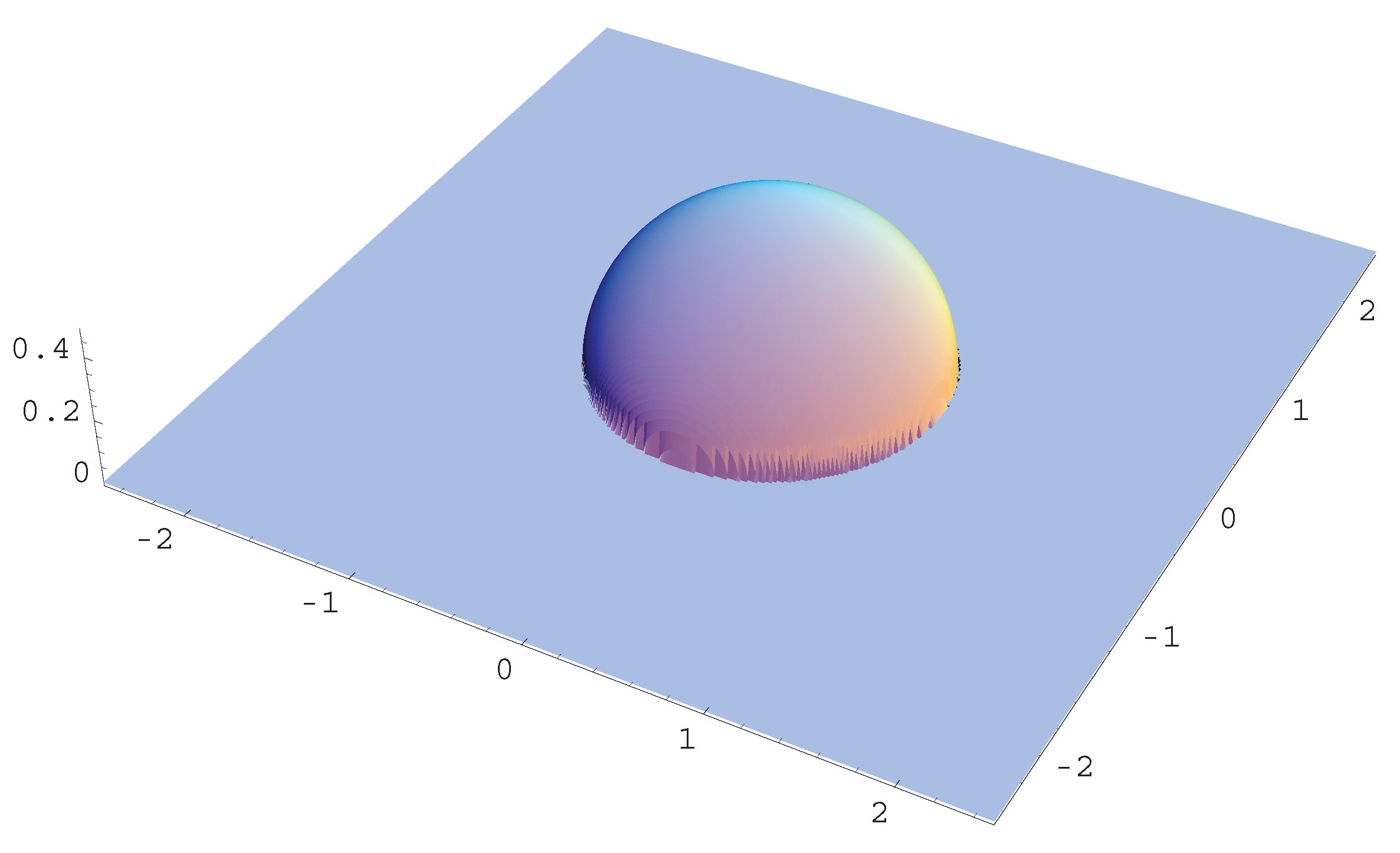
See the derivation for in Appendix 2. If the dimension d equals 1, then is a q-Gaussian distribution with . We remark that
in which is reduced to a d-variate Gaussian density when . The support of becomes an ellipsoid defined as
if . On the other hand, if , the density function (21) is written as
where
The d-variate t-distribution is defined by
cf. [20] for the extensive discussion. Assume that
Then we observe from (23) and (24) that
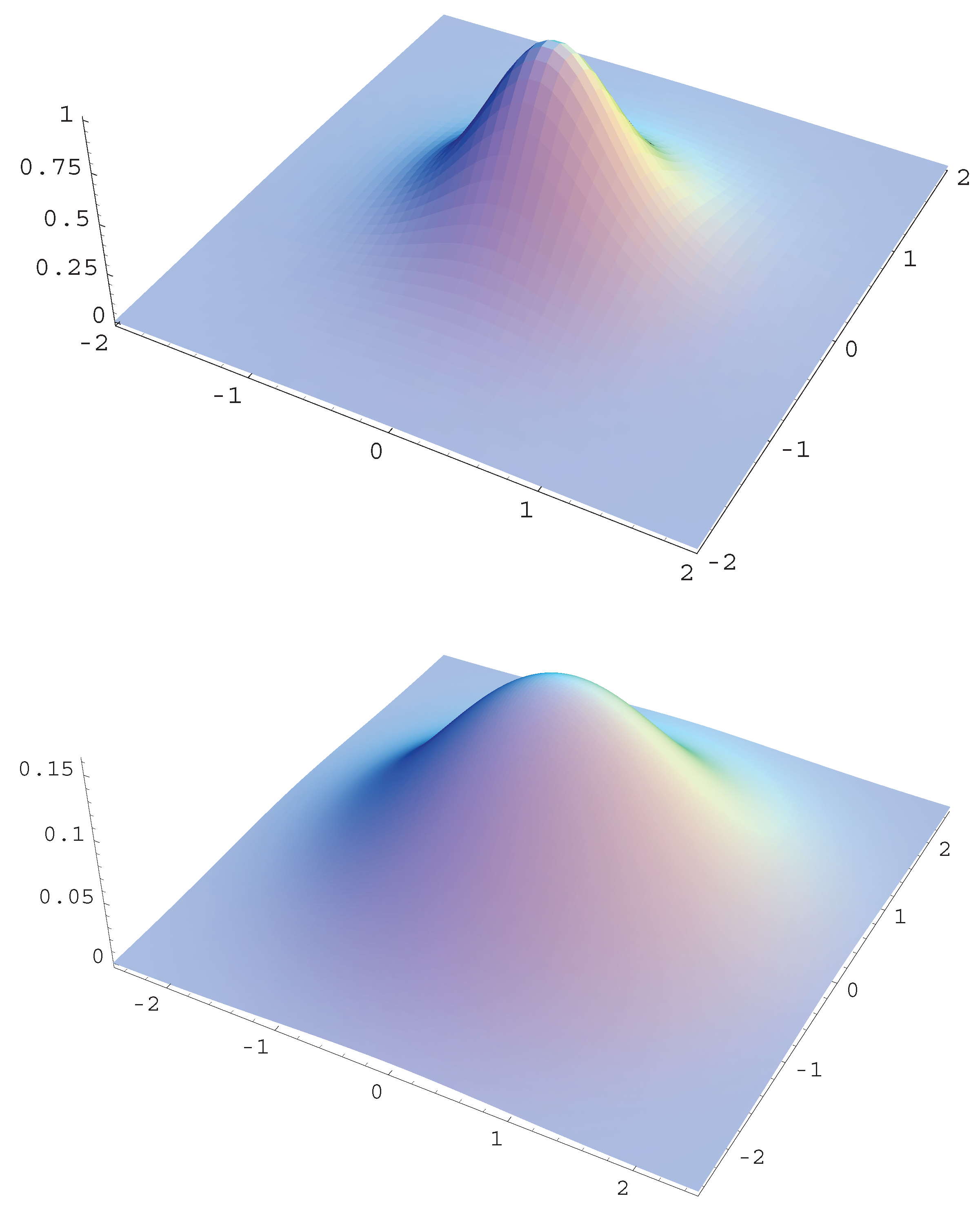
Accordingly, the density function with is a t-distribution. The distribution has elliptical contours on the Euclidean space for any , as shown in Figure 1 for typical cases of γ.
Figure 1.
t-distribution , Gaussian and Wigner distributions.

Let
which we call γ-model, where denotes the space of all symmetric, positive-definite matrices of order d. We confirm the mean and variance of the γ-model as follows.
Lemma. Under the model defined in (25) with the index ,
Proof. We need to consider a family of escort distributions. In the model we can define the escort distribution as
where and is the normalizing factor. Hence,
Here we define alternative parameter to the original parameter Σ by the transform
and so that the inverse transform is given by
noting that . Thus, we get a canonical form of (26) as
By analogy of the discussion for an exponential family we have the following expression for the braced term in (30) as
A property of the escort distribution suggests moment formulae for the distribution (25) as follows: We have an identity
which implies that
which concludes that
Similarly,
which is
which concludes that
because of the relation of and Σ as observed in (29). The proof is complete. ☐
Remark 3. The canonical form (30) of the escort distribution (26) plays an important role on the proof of Lemma. Basically we can write the canonical form of (21), however it is not known any link to distributional properties like a case of exponential family.
Remark 4. In Equation (31) the function
is viewed as a potential function in the Fenchel convex duality, where
cf. [21,22] for the covariance structure model.
From Lemma we observe that . Next we show that the distribution with density maximizes the γ-entropy over the space , where is defined in (2).
Theorem 2.
(i). If , then
where is defined in (20).
(ii). If , then
where
with being .
Proof. By the definition of , we see from Lemma that for any . This leads to
for any f in , which implies that
Hence
which is nonnegative as discussed in (4). This concludes (34). Similarly, we observe that (36) holds for any and any f in since the support of f includes that of . This concludes (35). ☐
We would like to elucidate a similar structure for the statistical inference by the minimum projective cross entropy in which the data set is assumed to follow the model . We recall (8) from the relation of the projective cross entropy with the escort distribution
When we have got data to be fitted to the model , the loss function is
where defined in (21). The γ-estimator is defined by
see the general definition (7). It follows from the canonical form defined in (30) with the canonical parameter defined in (28) that
where and ω are defined in (17) and (33), and is the normalizing factor defined in (27). Here we note that if , then the parameter must be assumed to be in , where
We note that and since
Accordingly, we observe the argument similar to (19) for the MLE. The projective divergence defined in (3) equals the difference of the γ-loss functions as
which is nonnegative with equality if and only if . See the discussion after equation (10). In this way, we can summarize the above discussion as follows:
Theorem 3. Let be a random sample from a γ-model defined in (21). Then the γ-estimator defined in (7) for is , where is defined in (17).
Proof. Let us give another proof. The estimating system is given by
which is equivalent to
because of the relation of into Σ as given in (29). Thus, we also attain the conclusion In this way, we obtain the solution of the equation system defined by (40) via the parameter using the relation of the escort distribution with the loss function (37). ☐
Remark 5. Consider the location model with the location parameter μ, where Σ is known in Theorem 3. Then we easily see that the γ-estimator for μ is . What about the reverse statement? We observe that if the γ-estimator for μ is with the sample size , then the model is the γ-model, with the known Σ. The proof is parallel to that of Theorem 2 given in [17]. In fact, we conclude that the model density function satisfies that
where a and b are constants.
Remark 6. If we look at jointly Theorem 2 and 3, then
since . Both sides of (41) associate with inequalities (39) and (36) on γ-divergence in separate discussion.
Remark 7. The derivation of the γ-estimator in Theorem 3 is provided by the canonical parameter of the escort distribution as given in (28). Here we directly calculate the gradient of the loss with respect to Σ as follows:
Therefore we observe that if we put and , then
The bracketed term of (42) is given by
which concludes that if , then . This is a direct proof for Theorem 3, but it would accompany with a heuristic discussion for the substitution of into .
4. Concluding Remarks
We explored the elegant property (39), the empirical Pythagoras relation between the γ-model and γ-estimator, in the sense that (39) directly shows Theorem 3 without any differential calculus. Another elegant expression is in the minimax game between Nature and a decision maker, see [23]. Consider the space defined in (20). The intersection of the γ-model (21) and is a singleton , which is the minimax solution of
Consider different indices γ and which specify the γ-model and -estimator, respectively. Basically the -estimator is consistent under the γ-model for any choice of γ and . If we specifically fix for the model, that is, a Gaussian model, then the -estimator is shown to be qualitatively robust for any , see [16]. The degree of robustness is proportional to the value of with a trade for the efficiency. The -estimator for of the Gaussian model is given by the solution of
The weight function for the i-th observation becomes almost 0 when is an outlier. Alternatively, the classical robust method employs , that is, the MLE for the misspecified model or t-distribution model, see [24,25]. Thus, the different indices γ and work robust statistics in a dualistic manner.
This property is an extension of that associated between the exponential model and MLE, however, it is fragile in the sense that (19) does not hold if the indices in the γ-model and -estimator are slightly different. In practice, we find some difficulties for a numerical task for solving the MLE under the γ-model with because the support of the density depends on the parameter and the index γ. We discussed statistical and probabilistic properties on the model and estimation associated with the specific cross entropy. A part of properties discussed still holds for any cross entropy in a much wider class, which is investigated from the point of the Fenchel duality in [13,26].
Acknowledgements
We would like to express our thanks to two referees for their helpful comments and constructive suggestions.
References
- Tsallis, C. Possible generalization of Boltzmann-Gibbs statistics. J. Statist. Physics. 1988, 52, 479–487. [Google Scholar] [CrossRef]
- Tsallis, C. Introduction to Nonextensive Statistical Mechanics: Approaching a Complex World; Springer-Verlag: New York, NY, USA, 2009. [Google Scholar]
- Cichocki, A.; Cruces, S.; Amari, S. Families of alpha- beta- and gamma- divergences: Flexible and robust measures of similarities. Entropy 2010, 12, 1532–1568. [Google Scholar] [CrossRef]
- Cichocki, A.; Cruces, S.; Amari, S. Generalized alpha-beta divergences and their application to robust nonnegative matrix factorization. Entropy 2011, 13, 134–170. [Google Scholar] [CrossRef]
- Csiszàr, I. Information-type measures of difference of probability distributions and indirect observation. Studia Scientiarum Mathematicarum Hungarica 1967, 2, 229–318. [Google Scholar]
- Rèny, I.A. On measures of entropy and information. Proc. Fourth Berkeley Symp. Math. Statist. Prob. 1961, 1, 547–561. [Google Scholar]
- Tøpsoe, F. Some inequalities for information divergence and related measures of discrimination. IEEE Trans. Inform. Theor. 2000, 46, 1602–1609. [Google Scholar]
- Amari, S. Differential-geometrical methods in statistics. In Lecture Notes in Statistics; Springer-Verlag: New York, NY, USA, 1985; Volume 28. [Google Scholar]
- Amari, S.; Nagaoka, H. Methods of information geometry. In Translations of Mathematical Monographs; American Mathematical Society: Providence, RI, USA, 2000; Volume 191. [Google Scholar]
- Eguchi, S. Second order efficiency of minimum contrast estimators in a curved exponential family. Ann. Statist. 1983, 11, 793–803. [Google Scholar] [CrossRef]
- Eguchi, S. Geometry of minimum contrast. Hiroshima Math. J. 1992, 22, 631–647. [Google Scholar]
- Basu, A.; Harris, I.R.; Hjort, N.L.; Jones, M.C. Robust and efficient estimation by minimizing a density power divergence. Biometrika 1988, 85, 549–559. [Google Scholar] [CrossRef]
- Eguchi, S. Information divergence geometry and the application to statistical machine learning. In Information Theory and Statistical Learning; Emmert-Streib, F., Dehmer, M., Eds.; Springer: New York, NY, USA, 2008; pp. 309–332. [Google Scholar]
- Minami, M.; Eguchi, S. Robust blind source separation by beta-divergence. Neural Comput. 2002, 14, 1859–1886. [Google Scholar]
- Eguchi, S.; Kato, S. Entropy and divergence associated with power function and the statistical application. Entropy 2010, 12, 262–274. [Google Scholar] [CrossRef]
- Fujisawa, H.; Eguchi, S. Robust parameter estimation with a small bias against heavy contamination. J. Multivariate Anal. 2008, 99, 2053–2081. [Google Scholar] [CrossRef]
- Azzalini, A.; Genton, M.G. On Gauss’s characterization of the normal distribution. Bernoulli 2007, 13, 169–174. [Google Scholar] [CrossRef]
- Teicher, H. Maximum likelihood characterization of distributions. Ann. Math. Statist. 1961, 32, 1214–1222. [Google Scholar] [CrossRef]
- Amari, S.; Ohara, A. Geometry of q-exponential family of probability distributions. Entropy 2011, 13, 1170–1185. [Google Scholar] [CrossRef]
- Kotz, S.; Nadarajah, S. Multivariate T Distributions and Their Applications; Cambridge University Press: Cambridge, UK, 2004. [Google Scholar]
- Eguchi, S. A differential geometric approach to statistical inference on the basis of contrast functionals. Hiroshima Math. J. 1985, 15, 341–391. [Google Scholar]
- Wakaki, H.; Eguchi, S.; Fujikoshi, Y. A class of tests for general covariance structure. J. Multivariate Anal. 1990, 32, 313–325. [Google Scholar] [CrossRef]
- Grünwald, P.D.; Dawid, A.P. Game theory, maximum entropy, minimum discrepancy, and robust Bayesian decision theory. Ann. Statist. 2004, 32, 1367–1433. [Google Scholar]
- Kent, J.T.; Tyler, D.E. Redescending M-estimates of multivariate location and scatter. Ann. Statist. 1991, 19, 2102–2119. [Google Scholar] [CrossRef]
- Marrona, R.A. Robust M-estimators of multivariate location and scatter. Ann. Statist. 1976, 4, 51–67. [Google Scholar] [CrossRef]
- Eguchi, S. Information geometry and statistical pattern recognition. Sugaku Exposition 2006, 19, 197–216. [Google Scholar]
Appendix 1
Appendix 2
First, we give the formula for in (22) when . Let
where The integral is rewritten as
where . It is expressed in polar coordinates as
where is the surface area of the unit sphere of dimension, that is,
Since the integral in (43) is expressed by a beta function, we have
Second, we give the formula when The argument similar to the above
where . It is expressed in polar coordinates as
which leads that
© 2011 by the authors; licensee MDPI, Basel, Switzerland. This article is an open access article distributed under the terms and conditions of the Creative Commons Attribution license (http://creativecommons.org/licenses/by/3.0/.)
Share and Cite
MDPI and ACS Style
Eguchi, S.; Komori, O.; Kato, S. Projective Power Entropy and Maximum Tsallis Entropy Distributions. Entropy 2011, 13, 1746-1764. https://doi.org/10.3390/e13101746
AMA Style
Eguchi S, Komori O, Kato S. Projective Power Entropy and Maximum Tsallis Entropy Distributions. Entropy. 2011; 13(10):1746-1764. https://doi.org/10.3390/e13101746
Chicago/Turabian StyleEguchi, Shinto, Osamu Komori, and Shogo Kato. 2011. "Projective Power Entropy and Maximum Tsallis Entropy Distributions" Entropy 13, no. 10: 1746-1764. https://doi.org/10.3390/e13101746