1.2. Complex network descriptors
Degree and Degree Distribution The simplest and the most intensively studied one vertex characteristic is degree. Degree,
k, of a vertex is the total number of its connections. If we are dealing with a directed graph, in-degree,
, is the number of incoming arcs of a vertex. Out-degree,
is the number of its outgoing arcs. Degree is actually the number of nearest neighbors of a vertex. Total distributions of vertex degrees of an entire network,
,
(the in-degree distribution), and
(the out-degree distribution) are its basic statistical characteristics. We define
to be the fraction of vertices in the network that have degree
k. Equivalently,
is the probability that a vertex chosen uniformly at random has degree
k. Most of the work in network theory deals with cumulative degree distributions,
. A plot of
for any given network is built through a cumulative histogram of the degrees of vertices, and this is the type of plot used throughout this article (and often referred to just as “degree distribution”). Although the degree of a vertex is a local quantity, we shall see that a cumulative degree distribution often determines some important global characteristics of networks. Yet another important parameter measured from local data and affecting the global characterization of the network is average degree
. This quantity is measured by the equation:
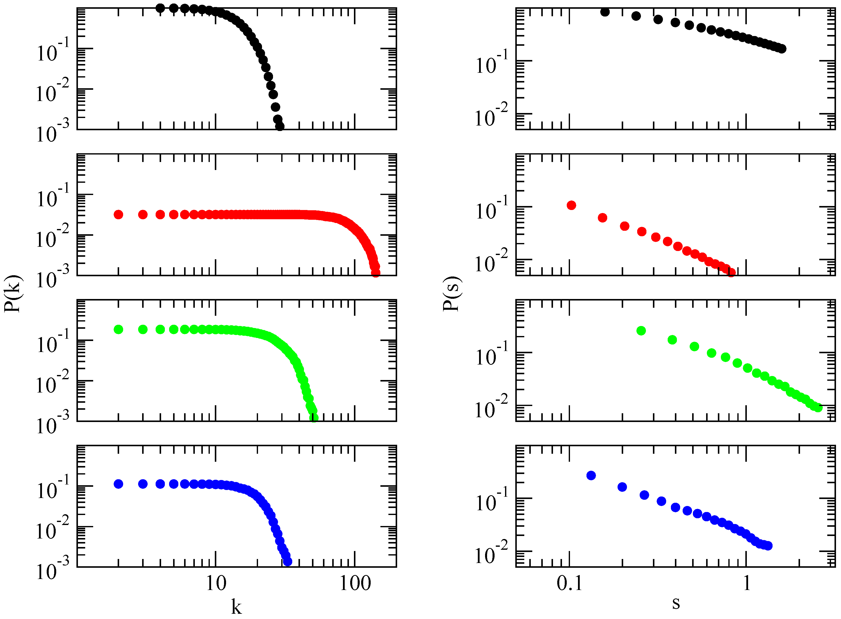
Strength Distribution In weighted networks the concept of degree of a node i () is not as important as the notion of strength of that node, , i.e., the sum over the nodes j in the of i, of weights from node i towards each of the nodes j in its neighborhood . In this type of network it is possible to measure the average strength with a slight modification of eq.1. On the other hand, it is also possible to plot the cumulative strength distribution , but it is important to make a good choice in the number of bins of the histogram (this depends on the particular distribution of weights for each network).
Shortest Path and Diameter For each pair of vertices i and j connected by at least one path, one can introduce the shortest path length, the so-called intervertex distance , the corresponding number of edges in the shortest path. Then one can define the distribution of the shortest-path lengths between pairs of vertices of a network and the average shortest-path length L of a network. The average here is over all pairs of vertices between which a path exists and over all realizations of a network. It determines the effective “linear size” of a network, the average separation of pairs of vertices. In a fully connected network, . Recall that shortest paths can also be measured in weighted networks, then the path’s cost equals the sum of the weights. One can also introduce the maximal intervertex distance over all the pairs of vertices between which a path exists. This descriptor determines the maximal extent of a network; the maximal shortest path is also referred to as the diameter (D) of the network.
Clustering Coefficient The presence of connections between the nearest neighbors of a vertex
i is described by its clustering coefficient. Suppose that a node (or vertex)
i in the network has
edges and they connect this node to
other nodes. These nodes are all neighbors of node
i. Clearly, at most
edges can exist among them, and this occurs when every neighbor of node
i connected to every other neighbor of node
i (number of loops of length 3 attached to vertex
i). The clustering coefficient
of node
i is then defined as the ratio between the number
of edges that actually exist among these
nodes and the total possible number:
Equivalently, the clustering coefficient of a node
i can be defined as the proportion of 3-cliques in which
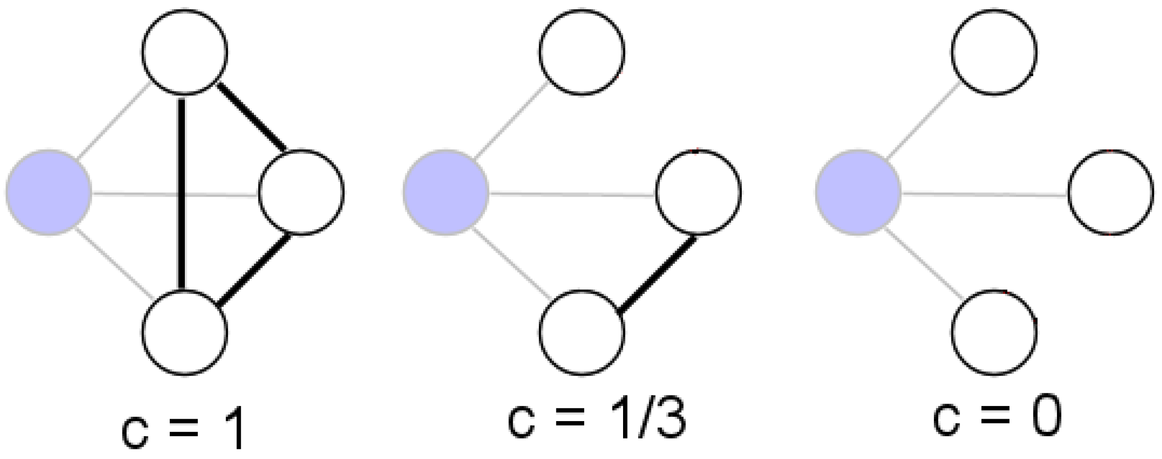
i participates. The clustering coefficient
C of the whole network is the average of
over all
i, see
Figure 1. Clearly,
; and
C = 1 if and only if the network is globally coupled, which means that every node in the network connects to every other node. By definition,
trees are graphs without loops,
i.e.,
.
The clustering coefficient of the network reflects the transitivity of the mean closest neighborhood of a network vertex, that is, the extent to which the nearest neighbors of a vertex are the nearest neighbors of each other [
6]. The notion of clustering was much earlier introduced in sociology [
27].
Centrality Measures Centrality measures are some of the most fundamental and frequently used measures of network structure. Centrality measures address the question, “Which is the most important or central node in this network?”, that is, the question whether nodes should all be considered equal in significance or not (whether exists some kind of hierarchy or not in the system). The existence of such hierarchy would then imply that certain vertices in the network are more central than others. There are many answers to this question, depending on what we mean by important. In this Section we briefly explore two centrality indexes (betweenness and eigenvector centrality) that are widely used in the network literature. Note however that betweenness or eigenvector centrality are not the only method to classify nodes’ importance. Within graph theory and network analysis, there are various measures of the centrality of a vertex within a graph that determine the relative importance of a vertex within the graph. For instance, besides betweenness, there are two other main centrality measures that are widely used in network analysis: degree centrality and closeness. The first, and simplest, is degree centrality, which assumes that the larger is the degree of a node, the more central it is. The closeness centrality of a vertex measures how easily other vertices can be reached from it (or the other way: how easily it can be reached from the other vertices). It is defined as the number of vertices minus one divided by the sum of the lengths of all geodesics from/to the given vertex.
a. Betweenness One of the first significant attempts to solve the question of node centrality is Freeman’s proposal (originally posed from a social point of view):
betweenness as a centrality measure [
28]. As Freeman points out, a node in a network is central to the extent that it falls on the shortest path between pairs of other nodes. In his own words, “suppose that in order for node
i to contact node
j, node
k must be used as an intermediate station. Node
k in such a context has a certain “responsibility” to nodes
i and
j. If we count all the minimum paths that pass through node
k, then we have a measure of the “stress” which node
k must undergo during the activity of the network. A vector giving this number for each node of the network would give us a good idea of stress conditions throughout the system” [
28]. Computationally, betweenness is measured according to the next equation:
with
as the number of shortest paths from
j to
k, and
the number of shortest paths from
j to
k that pass through vertex
i. Note that shortest paths can be measured in a weighted and/or directed network, thus it is possible to calculate this descriptor for any network [
29]. Commonly, betweenness is normalized by dividing through by the number of pairs of vertices not including
v, which is
. By means of normalization it is possible to compare the betweenness of nodes from different networks.
b. Eigenvector centrality A more sophisticated version of the degree centrality is the so-called eigenvector centrality [
30]. Where degree centrality gives a simple count of the number of connections a vertex has, eigenvector centrality acknowledges that not all connections are equal. In general, connections to people who are themselves influential will lend a person more influence than connections to less influential people. If we denote the centrality of vertex
i by
, then we can allow for this effect by making
proportional to the average of the centralities of
is network neighbors:
where
λ is a constant. Defining the vector of centralities
, we can rewrite this equation in matrix form as
and hence we see that
x is an eigenvector of the adjacency matrix with eigenvalue
λ. Assuming that we wish the centralities to be non-negative, it can be shown (using the Perron-Frobenius theorem) that
λ must be the largest eigenvalue of the adjacency matrix and
x the corresponding eigenvector. The eigenvector centrality defined in this way accords each vertex a centrality that depends both on the number and the quality of its connections: having a large number of connections still counts for something, but a vertex with a smaller number of high-quality contacts may outrank one with a larger number of mediocre contacts. In other words, eigenvector centrality assigns relative scores to all nodes in the network based on the principle that connections to high-scoring nodes contribute more to the score of the node in question than equal connections to low-scoring nodes.
Eigenvector centrality turns out to be a revealing measure in many situations. For example, a variant of eigenvector centrality is employed by the well-known Web search engine Google to rank Web pages, and works well in that context. Specifically, from an abstract point of view, the World Wide Web forms a directed graph, in which nodes are Web pages and the edges between them are hyperlinks [
31]. The goal of an Internet search engine is to retrieve an ordered list of pages that are relevant to a particular query. Typically, this is done by identifying all pages that contain the words that appear in the query, then ordering those pages using a measure of their importance based on their link structure. Although the details of the algorithms used by commercial search engines are proprietary, the basic principles behind the PageRank algorithm (part of Google search engine) are public knowledge [
32], and such algorithm relies on the concept of eigenvector centrality. Despite the usefulness of centrality measures, hierarchy detection and node’s role determination is not a closed issue. For this reason, other classifying techniques will be explored in subsequent Sections.
Degree-Degree correlation: assortativity It is often interesting to check for correlations between the degrees of different vertices, which have been found to play an important role in many structural and dynamical network properties. The most natural approach is to consider the correlations between two vertices connected by an edge. A way to determine the degree correlation is by considering the Pearson correlation coefficient of the degrees at both ends of the edges [
33,
34]
where
N is the total number of edges. If
the network is assortative; if
, the network is disassortative; for
there are no correlation between vertex degrees.
Degree correlations can be used to characterize networks and to validate the ability of network models to represent real network topologies. Newman computed the Pearson correlation coefficient for some real and model networks and discovered that, although the models reproduce specific topological features such as the power law degree distribution or the small-world property, most of them (e.g., the Erdös–Rényi and Barabási–Albert models) fail to reproduce the assortative mixing (
for the mentioned models) [
33,
34]. Further, it was found that the assortativity depends on the type of network. While social networks tend to be assortative, biological and technological networks are often disassortative. The latter property is undesirable for practical purposes, because assortative networks are known to be resilient to simple target attack, at the least.
There exist alternative definitions of degree-degree relations. Whereas correlation functions measure linear relations, information-based approaches measure the general dependence between two variables [
35]. Specially interesting is
mutual information provided by the expression
See the work by Solé and Valverde [
35] for details.
1.3. Network models
Regular Graphs Although regular graphs do not fall under the definition of complex networks (they are actually quite far from being complex, thus their name), they play an important role in the understanding of the concept of “small world”, see below. For this reason we offer a brief comment on them.
In graph theory, a regular graph is a graph where each vertex has the same number of neighbors,
i.e., every vertex has the same degree. A regular graph with vertices of degree
k is called a
k-regular graph or regular graph of degree
k [
36].
Random Graphs Before the burst of attention on complex networks in the decade of 1990s, a particularly rich source of ideas has been the study of random graphs, graphs in which the edges are distributed randomly. Networks with a complex topology and unknown organizing principles often appear random; thus random-graph theory is regularly used in the study of complex networks. The theory of random graphs was introduced by Paul Erdös and Alfréd Rényi [
15,
37,
38] after Erdös discovered that probabilistic methods were often useful in tackling problems in graph theory. A detailed review of the field is available in the classic book of Bollobás [
39]. Here we briefly describe the most important results of random graph theory, focusing on the aspects that are of direct relevance to complex networks.
a. The Erdös–Rényi Model In their classic first article on random graphs, Erdös and Rényi define a random graph as
N labeled nodes connected by
n edges, which are chosen randomly from the
possible edges [
15].
In a random graph with connection probability
p the degree
of a node
i follows a binomial distribution with parameters
and
p:
This probability represents the number of ways in which
k edges can be drawn from a certain node. To find the degree distribution of the graph, we need to study the number of nodes with degree
k,
. Our main goal is to determine the probability that
takes on a given value,
. According to equation 9, the expectation value of the number of nodes with degree
k is
with
The distribution of the
values,
, approaches a Poisson distribution,
Thus the number of nodes with degree
k follows a Poisson distribution with mean value
. Although random graph theory is elegant and simple, and Erdös and other authors in the social sciences, like Rapoport [
40,
41,
42,
43], believed it corresponded fundamental truth, reality interpreted as a network by current science is not aleatory. The established links between the nodes of various domains of reality follow fundamental natural laws. Despite some edges might be randomly set up, and they might play a non-negligible role, randomness is not the main feature in real networks. Therefore, the development of new models to capture real-life systems’ features other than randomness has motivated novel developments. Specially, two of these new models occupy a prominent place in contemporary thinking about complex networks. Here we define and briefly discuss them.
b. Watts–Strogatz small-world network In simple terms, the small-world concept describes the fact that despite their often large size, in most networks there is a relatively short path between any two nodes. The distance between two nodes is defined as the number of edges along the shortest path connecting them. The most popular manifestation of small worlds is the “six degrees of separation” concept, uncovered by the social psychologist Stanley Milgram [
4,
5], who concluded that there was a path of acquaintances with a typical length of about six between most pairs of people in the United States. This feature (short path lengths) is also present in random graphs. However, in a random graph, since the edges are distributed randomly, the clustering coefficient is considerably small. Instead, in most, if not all, real networks the clustering coefficient is typically much larger than it is in a comparable random network (
i.e., same number of nodes and edges as the real network). Beyond Milgram’s experiment, it was not until 1998 that Watts and Strogatz’ work [
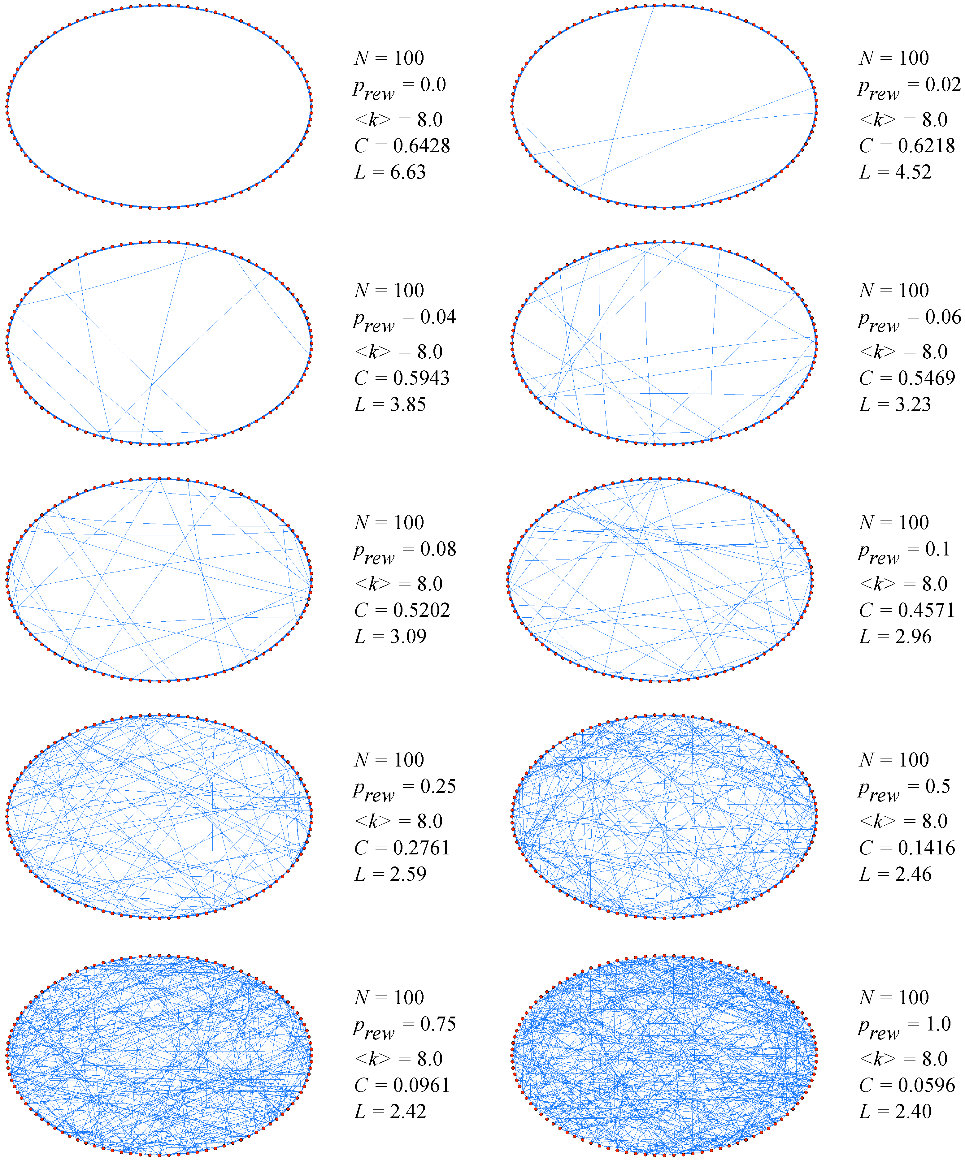
6] stimulated the study of such phenomena. Their main discovery was the distinctive combination of high clustering with short characteristic path length, which is typical in real-world networks (either social, biological or technological) that cannot be captured by traditional approximations such as those based on regular lattices or random graphs. From a computational point of view, Watts and Strogatz proposed a one-parameter model that interpolates between an ordered finite dimensional lattice and a random graph. The algorithm behind the model is the following [
6]:
Start with order: Start with a ring lattice with N nodes in which every node is connected to its first k neighbors ( on either side). In order to have a sparse but connected network at all times, consider .
Randomize: Randomly rewire each edge of the lattice with probability p such that self-connections and duplicate edges are excluded. This process introduces long-range edges which connect nodes that otherwise would be part of different neighborhoods. By varying p one can closely monitor the transition between order (p=0) and randomness (p=1).
The simple but interesting result when applying the algorithm was the following. Even for a small probability of rewiring, when the local properties of the network are still nearly the same as for the original regular lattice and the average clustering coefficient does not differ essentially from its initial value, the average shortest-path length is already of the order of the one for classical random graphs (see
Figure 2).
As discussed in [
44], the origin of the rapid drop in the average path length
L is the appearance of shortcuts between nodes. Every shortcut, created at random, is likely to connect widely separated parts of the graph, and thus has a significant impact on the characteristic path length of the entire graph. Even a relatively low fraction of shortcuts is sufficient to drastically decrease the average path length, yet locally the network remains highly ordered. In addition to a short average path length, small-world networks have a relatively high clustering coefficient. The Watts–Strogatz model (SW) displays this duality for a wide range of the rewiring probabilities
p. In a regular lattice the clustering coefficient does not depend on the size of the lattice but only on its topology. As the edges of the network are randomized, the clustering coefficient remains close to
C(0) up to relatively large values of
p.
Scale-Free Networks Certainly, the SW model initiated a revival of network modeling in the past few years. However, there are some real-world phenomena that small-world networks can’t capture, the most relevant one being evolution. In 1999, Barabási and Albert presented some data and formal work that has led to the construction of various scale-free models that, by focusing on the network dynamics, aim to offer a universal theory of network evolution [
16].
Several empirical results demonstrate that many large networks are scale free, that is, their degree distribution follows a power law for large k. The important question is then: what is the mechanism responsible for the emergence of scale-free networks? Answering this question requires a shift from modeling network topology to modeling the network assembly and evolution. While the goal of the former models is to construct a graph with correct topological features, the modeling of scale-free networks will put the emphasis on capturing the network dynamics.
In the first place, the network models discussed up to now (random and small-world) assume that graphs start with a fixed number N of vertices that are then randomly connected or rewired, without modifying N. In contrast, most real-world networks describe open systems that grow by the continuous addition of new nodes. Starting from a small nucleus of nodes, the number of nodes increases throughout the lifetime of the network by the subsequent addition of new nodes. For example, the World Wide Web grows exponentially in time by the addition of new web pages.
Second, network models discussed so far assume that the probability that two nodes are connected (or their connection is rewired) is independent of the nodes degree, i.e., new edges are placed randomly. Most real networks, however, exhibit preferential attachment, such that the likelihood of connecting to a node depends on the nodes degree. For example, a web page will more likely include hyperlinks to popular documents with already high degrees, because such highly connected documents are easy to find and thus well known.
a. The Barabási–Albert model These two ingredients, growth and preferential attachment, inspired the introduction of the Barabási–Albert model (BA), which led for the first time to a network with a power-law degree distribution. The algorithm of the BA model is the following:
It is specially in step (1) of the algorithm that the scale-free model captures the dynamics of a system. The power-law scaling in the BA model indicates that growth and preferential attachment play important roles in network development. However, some question arise when considering step (2): admitting that new nodes’ attachment might be preferential, is there only one equation (specifically, the one mentioned here) that grasps such preference across different networks (social, technological, etc.)? Can preferential attachment be expressed otherwise?
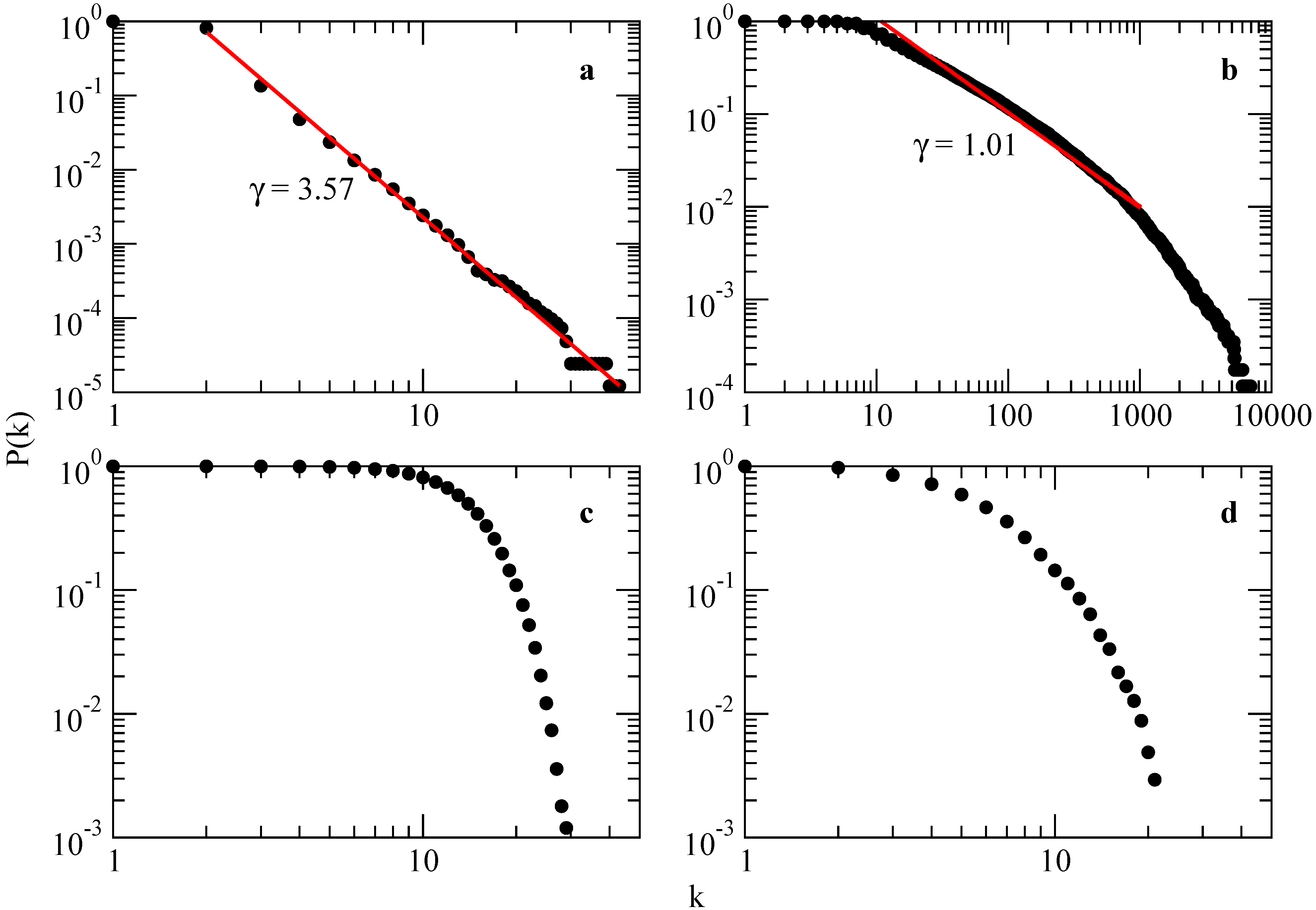
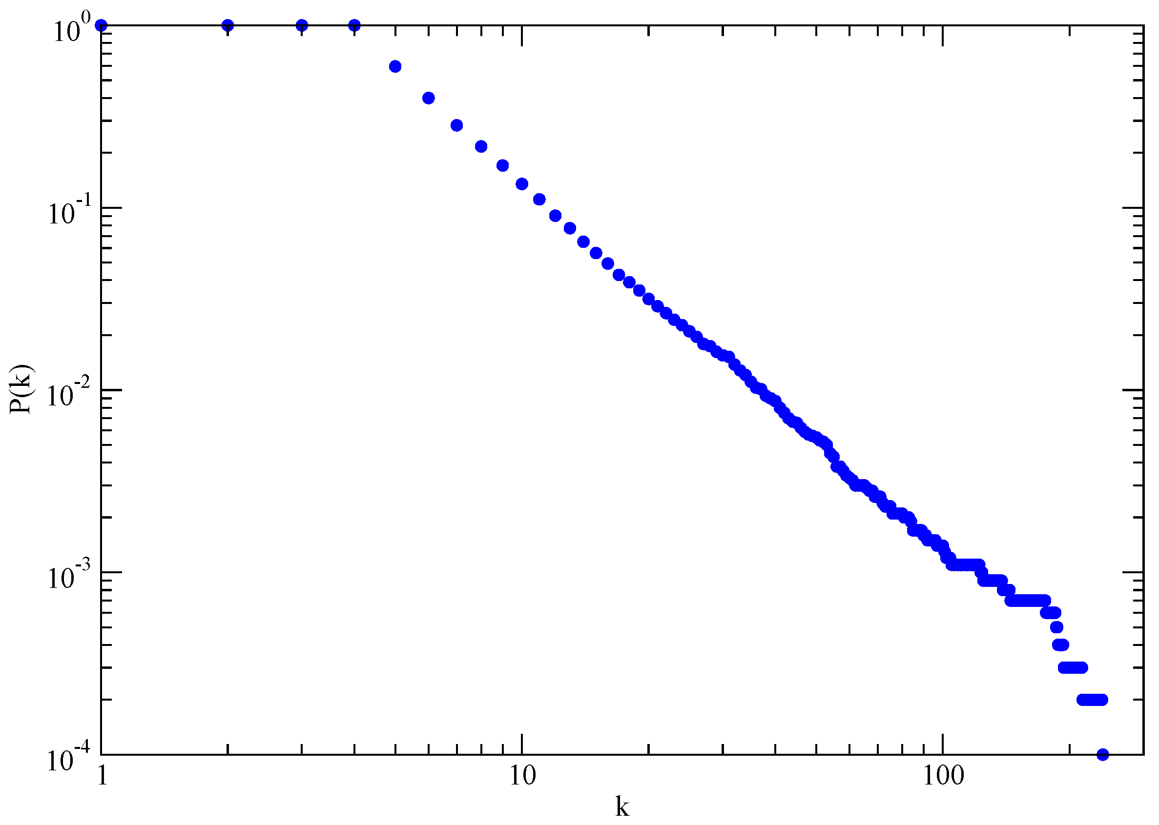
In the limit
(network with infinite size), the BA model produces a degree distribution
, with an exponent
, see
Figure 3.
The average distance in the BA model is smaller than in a ER-random graph with same N, and increases logarithmically with N. Analytical results predict a double logarithmic correction to the logarithmic dependence . The clustering coefficient vanishes with the system size as . This is a slower decay than that observed for random graphs, , but it is still different from the behavior in small-world models, where C is independent of N.
b. Other SF models The BA model has attracted an exceptional amount of attention in the literature. In addition to analytic and numerical studies of the model itself, many authors have proposed modifications and generalizations to make the model a more realistic representation of real networks. Various generalizations, such as models with nonlinear preferential attachment, with dynamic edge rewiring, fitness models and hierarchically and deterministically growing models, can be found in the literature. Such models yield a more flexible value of the exponent γ which is restricted to in the original BA construction. Furthermore, modifications to reinforce the clustering property, which the BA model lacks, have also been considered.
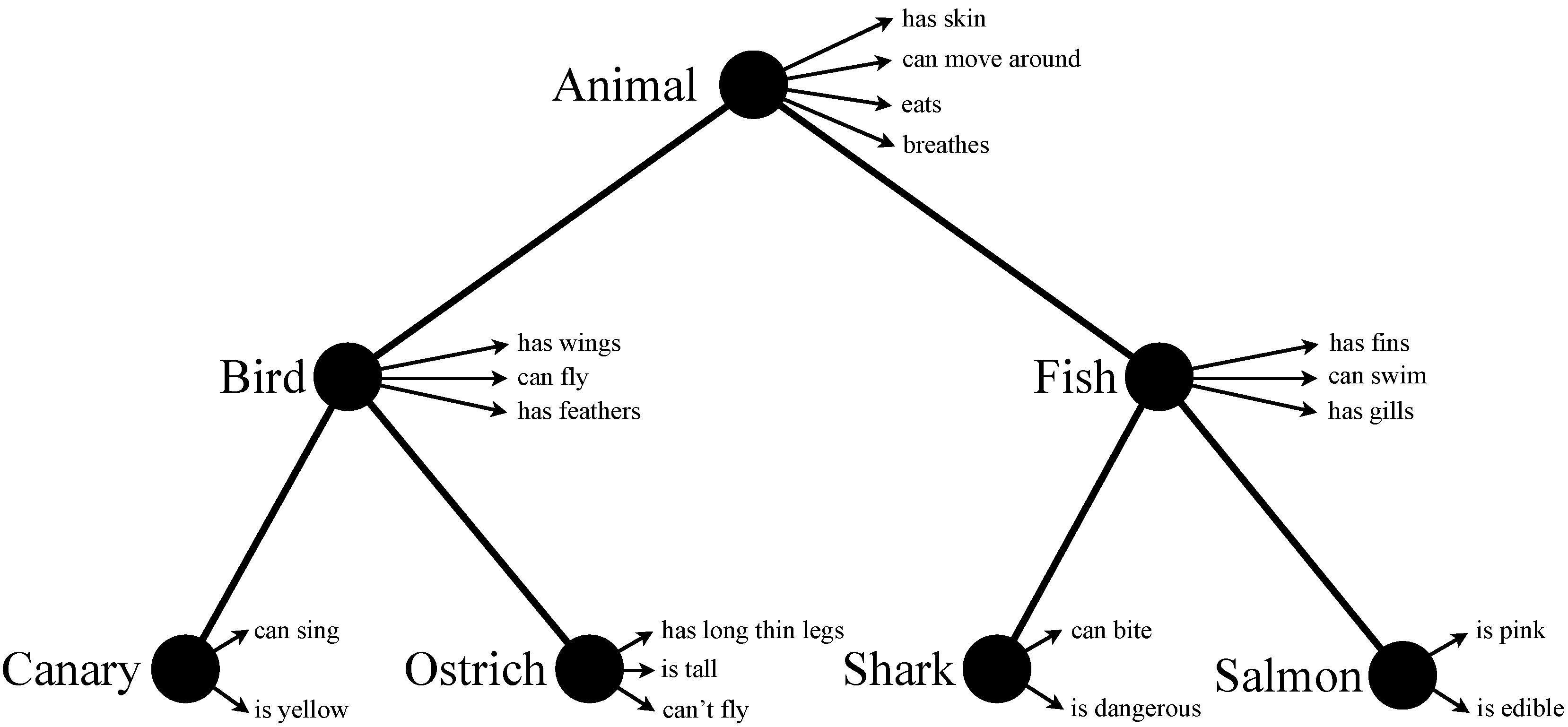
Among these alternative models we can find the
Dorogovtsev–Mendes–Samukhin (DMS) model, which considers a linear preferential attachment; or the
Ravasz–Barabási (RB) model, which aims at reproducing the hierarchical organization observed in some real systems (this makes it useful as an appropriate benchmark for multi-resolution community detection algorithms, see next Section and
Figure 4).
The
Klemm–Eguiluz (KE) model seeks to reproduce the high clustering coefficient usually found in real networks, which the BA model fails to reproduce [
45]. To do so, it describes the growth dynamics of a network in which each node of the network can be in two different states: active or inactive. The model starts with a complete graph of
m active nodes. At each time step, a new node
j with
m outgoing links is added. Each of the
m active nodes receives one incoming link from
j. The new node
j is then activated, while one of the
m active nodes is deactivated. The probability
that node
i is deactivated is given by
where
is the in-degree of node
i,
a is a positive constant and the summation runs over the set
of the currently active nodes. The procedure is iteratively repeated until the desired network size is reached. The model produces a scale-free network with
and with a clustering coefficient
when
. Since the characteristic path length is proportional to the network size (
) in the KE model, additional rewiring of edges is needed to recover the small-world property. Reference [
19] thoroughly discusses these and other models.
1.4. The mesoscale level
Research on networks cannot be solely the identification of actual systems that mirror certain properties from formal models. Therefore, the network approach has necessarily come up with other tools that enrich the understanding of the structural properties of graphs. The study of networks (or the methods applied to them) can be classified in three levels:
The study at the micro level attempts to understand the behavior of single nodes. Such level includes degree, clustering coefficient or betweenness and other parameters.
Meso level points at group or community structure. At this level, it is interesting to focus on the interaction between nodes at short distances, or classification of nodes, as we shall see.
Finally, macro level clarifies the general structure of a network. At this level, relevant parameters are average degree , degree distribution , average path length L, average clustering coefficient C, etc.
The first and third levels of topological description range from the microscopic to the macroscopic description in terms of statistical properties of the whole network. Between these two extremes we find the mesoscopic level of analysis of complex networks. In this level we describe an inhomogeneous connecting structure composed by subsets of nodes which are more densely linked, when compared to the rest of the network.
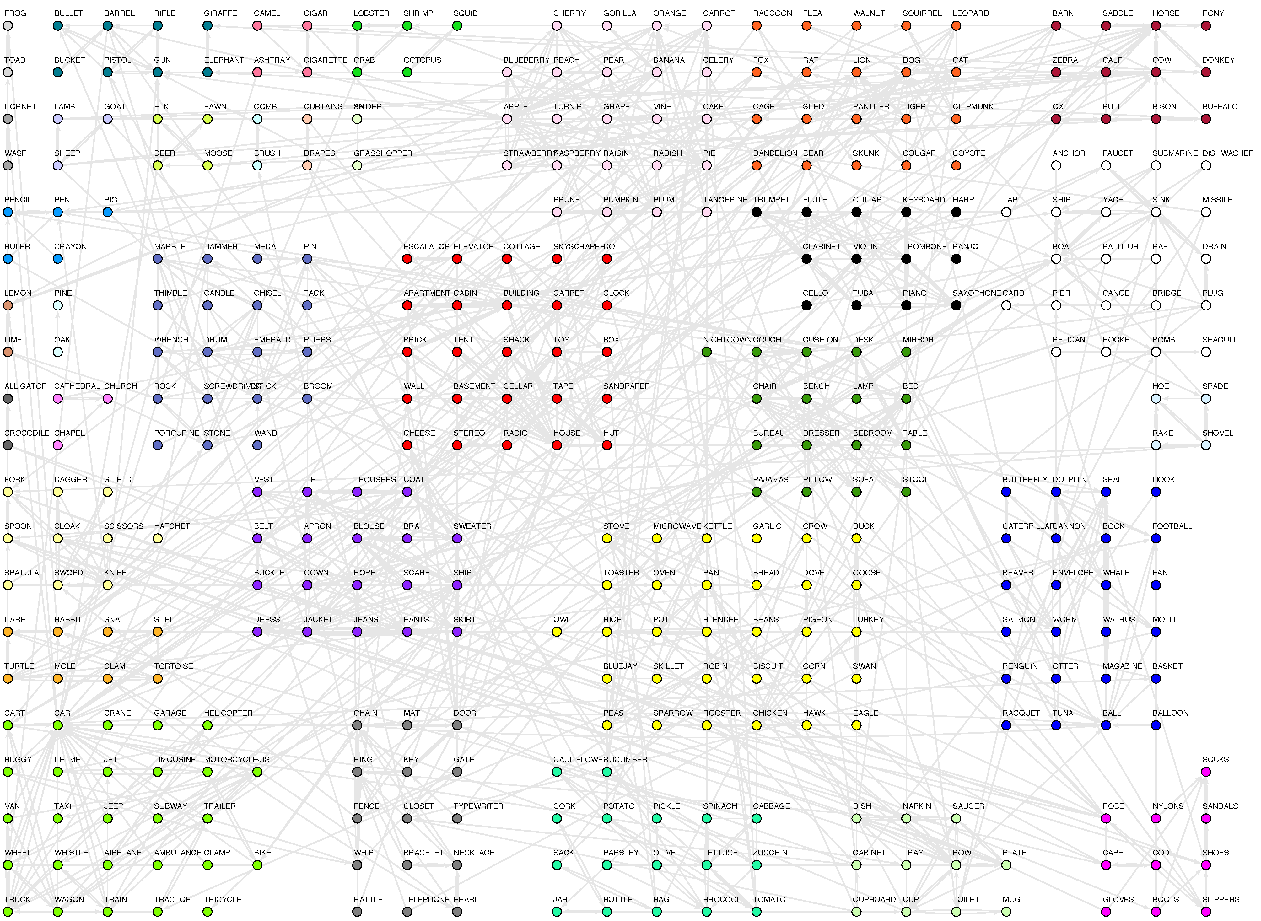
This mesoscopic scale of organization is commonly referred as
community structure. It has been observed in many different contexts, including metabolic networks, banking networks or the worldwide flight transportation network [
46]. Moreover, it has been proved that nodes belonging to a tight-knit community are more than likely to have other properties in common. For instance, in the world wide web community analysis has uncovered thematic clusters.
Whatever technique applied, the belonging of a node to one or another community cannot depend upon the “meaning” of the node, i.e., it can’t rely on the fact that a node represents an agent (sociology), a computer (the internet), a protein (metabolic network) or a word (semantic network). Thus communities must be determined solely by the topological properties of the network: nodes must be more connected within its community than with the rest of the network. Whatever strategy applied, it must be blind to content, and only aware of structure.
The problem of detection is particularly tricky and has been the subject of discussion in various disciplines. In real complex networks there is no way to find out,
a priori, how many communities can be discovered, but in general there are more than two, making the process more costly. Furthermore, communities may also be hierarchical, that is communities may be further divided into sub-communities and so on [
47,
48,
49]. Summarizing, it is not clear at what point a community detection algorithm must stop its classification, because no prediction can be made about the right level of analysis.
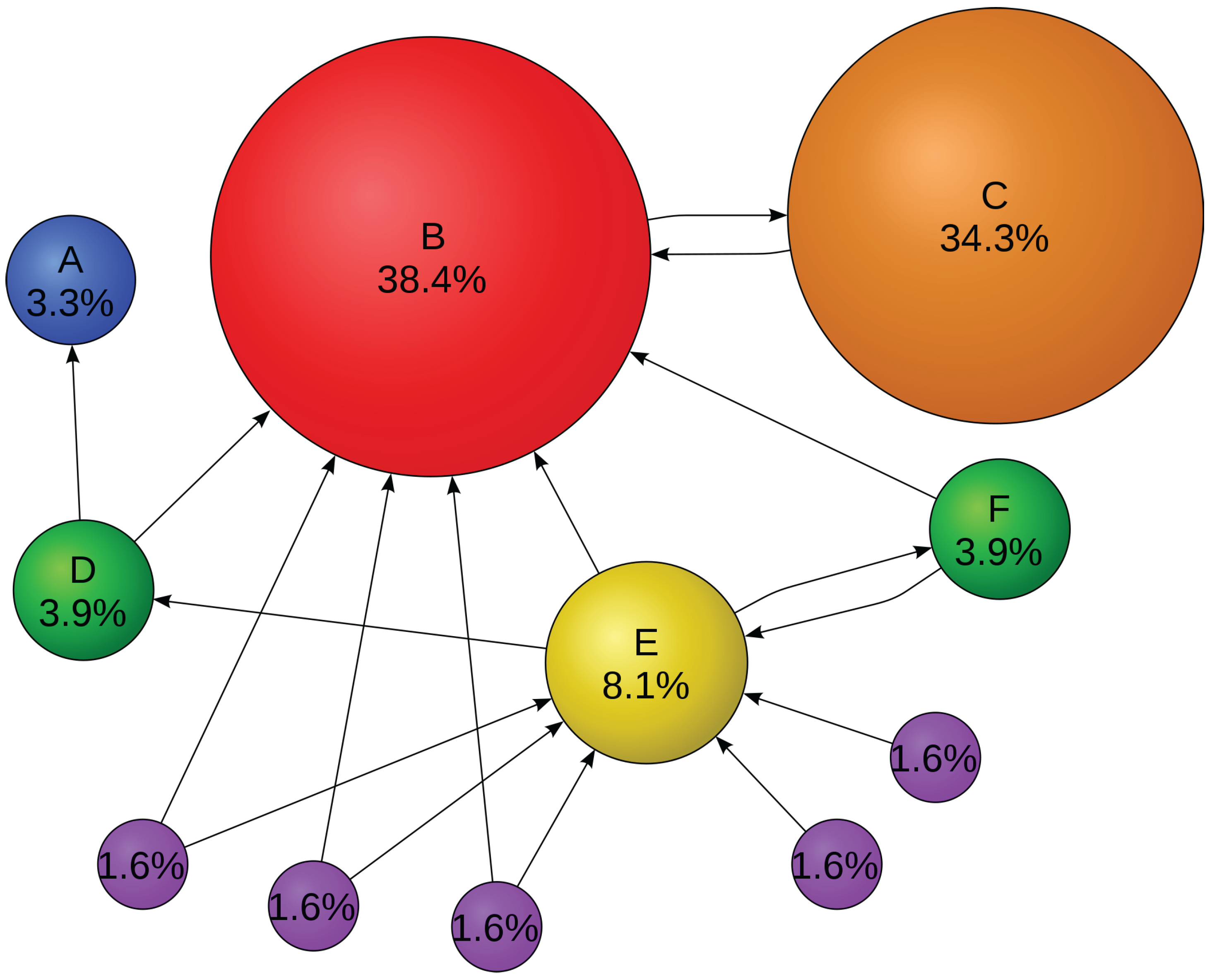
A simple approach to quantify a given configuration into communities that has become widely accepted was proposed in [
50]. It rests on the intuitive idea that random networks do not exhibit community structure. Let us imagine that we have an arbitrary network, and an arbitrary partition of that network into
communities. It is then possible to define a
x
size matrix
e where the elements
represent the fraction of total links starting at a node in partition
i and ending at a node in partition
j. Then, the sum of any row (or column) of
e,
corresponds to the fraction of links connected to
i. If the network does not exhibit community structure, or if the partitions are allocated without any regard to the underlying structure, the expected value of the fraction of links within partitions can be estimated. It is simply the probability that a link begins at a node in
i,
, multiplied by the fraction of links that end at a node in
i,
. So the expected number of intra-community links is just
. On the other hand we know that the real fraction of links exclusively within a community is
. So, we can compare the two directly and sum over all the communities in the graph.
This is a measure known as
modularity. Equation 15 has been extended to a directed and weighted framework, and even to one that admits negative weights [
51]. Designing algorithms which optimize this value yields good community structure compared to a null (random) model. The problem is that the partition space of any graph (even relatively small ones) is huge (the search for the optimal modularity value seems to be a
-hard problem due to the fact that the space of possible partitions grows faster than any power of the system size), and one needs a guide to navigate through this space and find maximum values. Some of the most successful heuristics are outlined in [
52,
53]. The first one relies on a genetic algorithm method (Extremal Optimization), while the second takes a greedy optimization (hill climbing) approach. Also, there exist methods to decrease the search space and partially relieve the cost of the optimization [
54]. In [
55] a comparison of different methods is developed, see also [
56].
Modularity-based methods have been extended to analyze the community structure at different resolution levels, thus uncovering the possible hierarchical organization of the mesoscale [
49,
57,
58].
With the methodological background developed in the previous
Section 1, it is now possible to turn to language. The following Sections are devoted to acknowledge the main achievements of a complex network approach to language and the cognitive processes associated to it.


