Reconsideration of Criteria and Modeling in Order to Optimize the Efficiency of Irreversible Thermomechanical Heat Engines

Abstract

The purpose of this work is to precise and complete one recently proposed in the literature and relative to a general criterion to maximize the first law efficiency of irreversible heat engines. It is shown that the previous proposal seems to be a particular case. A new proposal has been developed for a Carnot irreversible thermomechanical heat engine at steady state associated to two infinite heat reservoirs (hot source, and cold sink): this constitutes the studied system. The presence of heat leak is accounted for, with the most simple form, as is done generally in the literature. Irreversibility is modeled through ${\stackrel{.}{s}}_i$, created internal entropy rate in the converter (engine), and ${\stackrel{.}{s}}_T$, total created entropy rate in the system. Heat transfer laws are represented as general functions of temperatures. These concepts are particularized to the most common heat transfer law (linear one). Consequences of the proposal are examined; some new analytical results are proposed for efficiencies.

1. Introduction

Carnot is without doubt the precursor of the development in the field of Equilibrium Thermodynamics applied to machines, systems and processes; he introduced the concept of cycle, mainly the “Carnot cycle”. Finally he can be credited with being the originator of the notion of efficiency, an important concept in today’s world [1].

Finite Time Thermodynamics (F.T.T.) is associated with the work of Curzon and Ahlborn [2]; in that work, the authors observed that the efficiency at MAX(–W) becomes less than the Carnot limit. But this was first pointed out by Chambadal [3] and by Novikov [4] in 1957: the Chambadal-Novikov-Curzon-Ahlborn efficiency differs from that given by Carnot. These works have been continuously completed since; see for example [5,6,7,8,9].

It is well know that the first law efficiency of the Carnot engine in the equilibrium thermodynamics limit is:

$${\eta }_C=1-\frac{T_{SC}}{T_{SH}}$$

(1)

The CNCA efficiency delivered by an endoreversible Carnot engine in contact with two infinite heat reservoirs at T_SH (hot source) and T_SC (cold sink) is:

$${\eta }_C\left(MAX\left(-\stackrel{.}{W}\right)\right)=1-\sqrt{\frac{T_{SC}}{T_{SH}}}$$

(2)

The corresponding power versus efficiency curve has been repeated in Figure 1, and published in a recent paper [10]: Figure 1(a) corresponds to the endoreversible case. In fact it is well known that real engines and systems have a loop-shaped power-efficiency curve [see Figure 1(b)], as was recognized first from an experimental point of view by Gordon [11].

Figure 1. a. (left) Variation of the Carnot endoreversible engine power versus efficiency. b. (right) Variation of the Carnot endoreversible engine power versus efficiency in presence of thermal losses.

Figure 1. a. (left) Variation of the Carnot endoreversible engine power versus efficiency. b. (right) Variation of the Carnot endoreversible engine power versus efficiency in presence of thermal losses.

Numerous works are concerned with heat leak model [12,13,14], internal irreversibility model [15,16,17], and irreversible model with heat resistance, heat leakage and internal irreversibility with different heat transfer laws [18,19,20,21].

Models have been developed to account for the loop shaped form [see Figure 1(b)]: it includes heat losses, or irreversibility trough an entropy ratio [22], or more recently through a created entropy rate $\stackrel{.}{s}$ [23]. This second method is preferred because connected to the entropy analysis [24].

A $MAX{\eta }_I$, maximum efficiency according to first law appears, that is smaller than ${\eta }_C$, and occurs at point C, thus reducing the high efficiency zone of the engine. In a recent paper [25] Aragon-Gonzales et al. propose a general criterion to maximize efficiencies of several heat engines (Brayton engine; Carnot engine). This criterion seems to be a particular one that cannot be applied as a general criterion to all kind of heat engines.

We intend to demonstrate this fact, in the present paper, by two ways: first, we apply the proposal of the authors, to some cases of irreversible Carnot cycle, as done in Section 4 of the referenced paper [25], and we will observe that, it does not fit the hypothesis.

Secondly, we develop always for the irreversible Carnot cycle, a general model, under the same main conditions as used in Aragon-Gonzales et al. paper. We deduce the new general method relative to first law efficiency of a Carnot engine optimization.

We apply this last method to some particular and realistic models corresponding to what is done in the literature [26]. This provides some new analytical results concerning first law efficiency upper bound that will be commented: the optimum efficiency differs from the one relative to minimum of total created entropy rate.

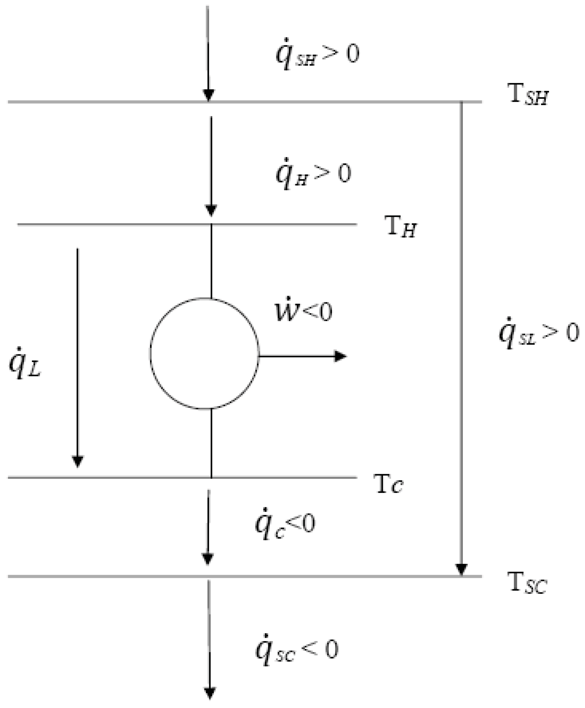
2. General Model of the CARNOT Irreversible Engine

The Carnot irreversible engine could be defined as a thermomechanical engine (converter) in contact with two infinite heat reservoirs (hot and cold thermostats); the engine and the two thermostats constitute the studied system. The authors of Reference [25] consider a finite-time thermodynamics approach, that could be discussed; we however prefer to use steady state modeling, but also with irreversibilities and heat losses. The scheme of the system is proposed in Figure 2.

Figure 2. Scheme of the system comprising the irreversible Carnot engine.

Figure 2. Scheme of the system comprising the irreversible Carnot engine.

It can be seen that the thermal loss used by the authors of Reference [25] corresponds to general actual modelling: a thermal short circuit, between the hot source at temperature T_SH, and the cold sink at temperature T_SC, generally the ambient temperature. The corresponding heat flux is:

$${\stackrel{.}{q}}_{SL}=K_{SL}.f_{SL}\left(T_{SH},T_{SC}\right)$$

(3)

where:

• K_SL, generalized heat loss conductance,
• f_SL(T_SH, T_SC), function characterizing the heat transfer.

It is to be noted that, in the material of the engine too, it must exist conductive heat loss, between the hot part and the cold part:

$${\stackrel{.}{q}}_L=K_L.f_L\left(T_H,T_C\right)$$

(4)

But, we can suppose that these heat losses correspond to internal dissipation in the engine converter, and participate of the internal entropy flux of the engines ${\stackrel{.}{s}}_i$ [see Relation (11) hereafter]. According to this assumption, we could summarize saying that the heat losses in the system are assumed to occur between the maximum temperature T_SH, and the minimum temperature T_SC of the system, through an equivalent heat transfer conductance K_SL [see Relation (3)].

Using thermodynamical convention (see Figure 2), it comes for the used heat rate at the source ${\stackrel{.}{q}}_{SH}$, and rejected heat rate at the sink:

$${\stackrel{.}{q}}_{SH}={\stackrel{.}{q}}_H+{\stackrel{.}{q}}_{SL}$$

(5)

$${\stackrel{.}{q}}_{SC}={\stackrel{.}{q}}_C-{\stackrel{.}{q}}_{SL}$$

(6)

In fact, these two definitions are completed by the two heat transfer laws between source and hot side of the engine at temperature T_H, and between cold side of the engine at T_C and the sink [26]:

$${\stackrel{.}{q}}_H=K_H.f_H\left(T_{SH}.T_H\right)$$

(7)

$${\stackrel{.}{q}}_C=K_C{f}_C\left(T_{SC},T_C\right)$$

(8)

Applying first law of thermodynamics to the system it becomes:

$$\stackrel{.}{w}+{\stackrel{.}{q}}_{SH}+{\stackrel{.}{q}}_{SC}=0$$

(9)

Applying second law of thermodynamics to the system it becomes:

$$\frac{{\stackrel{.}{q}}_{SH}}{T_{SH}}+\frac{{\stackrel{.}{q}}_{SC}}{T_{SC}}+{\stackrel{.}{s}}_T=0$$

(10)

where ${\stackrel{.}{s}}_T$ represents the total entropy rate of the system due to all irreversibilities. It differs from the one use by Aragon-Gonzales et al. [25], that corresponds to the entropy balance applied to the converter as:

$$\frac{{\stackrel{.}{q}}_H}{T_H}+\frac{{\stackrel{.}{q}}_C}{T_C}+{\stackrel{.}{s}}_i=0$$

(11)

Further , the authors use, as is traditional in the literature, an irreversibility ratio I (parameter); the interest of using, the entropy rate ${\stackrel{.}{s}}_i$ has been exposed in recent paper [10], and we move to this entropy flux method preferably; for generality, we choose to express ${\stackrel{.}{s}}_T$ as a function of temperatures T_SH, T_SC, T_H, T_C and ${\stackrel{.}{s}}_i$ as a function of (T_H, T_C):

$${\stackrel{.}{s}}_T=f_{ST}\left(T_{SH},T_{SC},T_H,T_C\right)$$

(12)

$${\stackrel{.}{s}}_i=f_{Si}\left(T_H,T_C\right)$$

(13)

The justification of the form of ${\stackrel{.}{s}}_T$, is easily obtained, using (10, 11, 12, 13). Effectively it appears that:

$${\stackrel{.}{s}}_T={\stackrel{.}{s}}_i+{\stackrel{.}{q}}_H\left(\frac{1}{T_H}-\frac{1}{T_{SH}}\right)+{\stackrel{.}{q}}_C\left(\frac{1}{T_C}-\frac{1}{T_{SC}}\right)-{\stackrel{.}{q}}_{SL}\left(\frac{1}{T_{SH}}-\frac{1}{T_{SC}}\right)$$

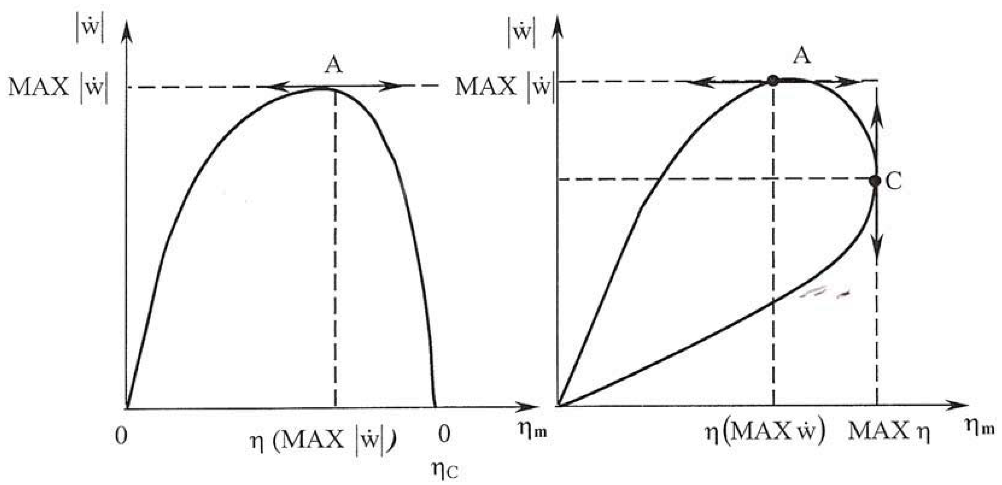
3. Maximum Efficiency Criterion

We focus here on the system first law efficiency ${\eta }_{IS}$:

$${\eta }_{IS}=\frac{-\stackrel{.}{w}}{{\stackrel{.}{q}}_{SH}}$$

(14)

It is easy to eliminate $-\stackrel{.}{w}$ through (9):

$${\eta }_{IS}=1+\frac{{\stackrel{.}{q}}_{SC}}{{\stackrel{.}{q}}_{SH}}=1+\frac{K_C.f_C-{\stackrel{.}{q}}_{SL}}{K_H.f_H+{\stackrel{.}{q}}_{SL}}$$

(15)

In the same way, it is possible to obtain the converter (or engine) first law efficiency; it corresponds to:

$${\eta }_{IE}=1+\frac{{\stackrel{.}{q}}_C}{{\stackrel{.}{q}}_H}=1+\frac{K_C{f}_C}{K_H{f}_H}$$

(16)

Using the entropy balance of the engine, it is easy to show that ${\eta }_{IE}$ could also be expressed as:

$${\eta }_{IE}=1-\frac{T_C}{T_H}-\frac{T_C{\stackrel{.}{s}}_i}{{\stackrel{.}{q}}_H}$$

(17)

correspondingly, ${\eta }_{IS}$ could be expressed as:

$${\eta }_{IS}=1-\frac{T_{SC}}{T_{SH}}-\frac{T_{SC}{\stackrel{.}{s}}_T}{{\stackrel{.}{q}}_{SH}}$$

(18)

The two last relations suggest that the first law efficiency of the system is bounded by the classical Carnot efficiency associated to equilibrium thermodynamics, whereas the converter efficiency is bounded by the endoreversible efficiency, whatever the link with the source and sink. In case of a perfect (reversible) link, we recover the Carnot first law efficiency. Generally the published paper consider more the engine aspect, than the system one: we focus here on the system one.

Relation (18) indicates that the system efficiency depends on two functions ${\stackrel{.}{s}}_T$ and ${\stackrel{.}{q}}_{SH}$. So, for a designed system K_H, K_C, T_SH, T_SC are parameters, and T_H, T_C (or X_H = T_SH – T_H, X_C = T_SC – T_C) natural (generic) variables. But the two variables are connected through the entropy balance (10). There is only one degree of freedom as supposed in the paper of [25].

3.1. Developing the Criterion with the Degree of Freedom x

By derivation of (18), it comes:

$$\frac{d{\eta }_{IS}}{dx}=0=-\frac{T_{SC}}{{{\stackrel{.}{q}}_{SH}}^2}\left[\frac{\partial {\stackrel{.}{s}}_T}{\partial x}.{\stackrel{.}{q}}_{SH}-{\stackrel{.}{s}}_T\frac{\partial {\stackrel{.}{q}}_{SH}}{\partial x}\right]$$

We deduce a corresponding relation for the optimum system efficiency, more general than expression (2.2) of Aragon-Gonzales et al. paper:

$$OPT{\eta }_{IS}=1-\frac{T_{SC}}{T_{SH}}-T_{SC}\frac{\partial {\stackrel{.}{s}}_T/\partial x}{\partial {\stackrel{.}{q}}_{SH}/\partial x}, \text{with} x=x_{opt}$$

(19)

3.2. Developing the Criterion with Variationnal Calculus

The lagragian of the system L (T_H, T_C) is:

$$L=1+\frac{K_C{f}_C-{\stackrel{.}{q}}_{SL}}{K_H{f}_H+{\stackrel{.}{q}}_{SL}}+\lambda \text{}\left[\frac{K_H{f}_H+{\stackrel{.}{q}}_{SL}}{T_{SH}}+\frac{K_C{f}_C-{\stackrel{.}{q}}_{SL}}{T_{SC}}+f_{ST}\right]$$

By derivation, we obtain the equations system to solve with respect to (T_H, T_C, $\lambda$), and eliminating $\lambda$, the two equations in T_H, T_C, given hereafter:

$$\{\begin{array}{c}\frac{\left[\frac{K_H}{T_{SH}}{f}_{H,H}+f_{ST,H}\right]\left(K_H{f}_H+{\stackrel{.}{q}}_{SL}\right)}{K_H{f}_{H,H}}=-\frac{\left[\frac{K_C}{T_{SC}}{f}_{C,C}+f_{ST,C}\right]\left(K_C{f}_C-{\stackrel{.}{q}}_{SL}\right)}{K_C{f}_{C,C}}\\ \frac{K_H{f}_H+{\stackrel{.}{q}}_{SL}}{T_{SH}}+\frac{K_C-{\stackrel{.}{q}}_{SL}}{T_{SC}}+f_{ST}=0\end{array}$$

(20)

with the notation $f_{i,j}=\frac{\partial f_i}{{\partial }_{xj}}$.

The expression of the optimum system efficiency, is calculated using T_H*, T_C*, solutions of the given system in:

$${\eta }_{ISopt}=1-\frac{\frac{1}{T_{SH}}+\frac{f_{ST,H}}{K_H{f}_{H,H}}}{\frac{1}{T_{SC}}+\frac{f_{ST,C}}{K_C{f}_{C,C}}}$$

(21)

This result indicates that optimized efficiency depends only on first derivative of the heat transfer laws, on of the total entropy flux of the system. This result could be validated on the limit case of reversible system (${\stackrel{.}{s}}_T=0$ and $f_{ST,H}=f_{ST,C}=0$); we retrieve the equilibrium thermodynamics result: Carnot efficiency.

4. Some Results and Discussion

4.1. Conditions Suggested in Paper [25]

Are the conditions $\frac{{\partial }^2{\stackrel{.}{q}}_{SH}}{\partial x^2}<0$ and $\frac{{\partial }^2{\stackrel{.}{q}}_{SC}}{\partial x^2}=0$ realistic?

These conditions are checked for the Carnot thermomechanical system, for various heat transfer laws used in the literature and supposing the same law for the hot and cold side of the system.

4.1.1. Example 1: Linear Heat Transfer Laws

In this case ${\stackrel{.}{q}}_{SH}=K_H\left(K_{SH}-T_H\right)+{\stackrel{.}{q}}_{SL}$

$${\stackrel{.}{q}}_{SC}=K_C\left(K_{SC}-T_C\right)-{\stackrel{.}{q}}_{SL}$$

and the entropy constraint:

$$\frac{K_H\left(T_{SH}-T_H\right)}{T_{SH}}+\frac{K_C\left(T_{SC}-T_C\right)}{T_{SC}}+{\stackrel{.}{s}}_T=0$$

with ${\stackrel{.}{s}}_T=f_{ST}\left(T_H,T_C\right)$.

Choosing T_H as independent variable it comes:

$$\frac{d^2{\stackrel{.}{q}}_{SH}}{d{T_H}^2}=0;\frac{d^2{\stackrel{.}{q}}_{SC}}{d{T_H}^2}=-K_C\frac{d^2{T}_C}{d{T_H}^2}$$

with:

$$\frac{d{T}_C}{d{T}_H}=-\frac{\frac{K_H}{T_{SH}}-\frac{\partial {\stackrel{.}{s}}_T}{\partial T_H}}{\frac{K_C}{T_{SC}}-\frac{\partial {\stackrel{.}{s}}_T}{\partial T_C}}$$

$$\frac{d^2{T}_C}{d{T_H}^2}=-\frac{-\frac{{\partial }^2{\stackrel{.}{s}}_T}{\partial {T_H}^2}\left(\frac{K_C}{T_{SC}}-\frac{\partial {\stackrel{.}{s}}_T}{\partial T_C}\right)+\left(\frac{K_H}{T_{SH}}-\frac{\partial {\stackrel{.}{s}}_T}{\partial T_H}\right)\frac{{\partial }^2{\stackrel{.}{s}}_T}{\partial {T_C}^2}.\frac{d{T}_C}{d{T}_H}}{{\left(\frac{K_C}{T_{SC}}-\frac{\partial {\stackrel{.}{s}}_T}{\partial T_C}\right)}^2}$$

This last formula tends to prove that generally $\frac{{\partial }^2{\stackrel{.}{q}}_{SC}}{\partial {T_H}^2}\ne 0$, except if ${\stackrel{.}{s}}_T$ is a constant (non function of T_H, T_C), or a linear function of T_H, T_C.

4.1.2. Example 2: Generalized Convective Laws

In this case we move from variable T_i, to X_i according to:

$${\stackrel{.}{q}}_{SH}=K_H{X_H}^n>0$$

$${\stackrel{.}{q}}_{SC}={\left(-1\right)}^{n-1}{K}_C{X_C}^n<0$$

and the entropy constraint:

$$\frac{K_H{X_H}^n}{T_{SH}}+\frac{{\left(-1\right)}^n{K}_C{X_C}^n}{T_{SC}}+f_{ST}\left(X_H,X_C\right)=0$$

With X_H independent variables, it comes:

$$\frac{{\partial }^2{\stackrel{.}{q}}_{SH}}{\partial {X_H}^2}=n(n-1)K_H{X_H}^{n-2}>0$$

$$\frac{{\partial }^2{\stackrel{.}{q}}_{SC}}{\partial {X_H}^2}={\left(-1\right)}^{n-1}\left[n(n-1){X_C}^{n-2}{\left(\frac{d{X}_C}{d{X}_H}\right)}^2+n{X_C}^{n-1}\frac{d^2{X}_C}{d{X_H}^2}\right]$$

and:

$$\frac{d{X}_C}{d{X}_H}=-\frac{\frac{n{K}_H{X_H}^{n-1}}{T_{SH}}+f_{ST,H}}{{(-1)}^{n-1}\frac{n{K}_C{X_C}^{n-1}}{T_{SC}}+f_{ST,C}}$$

The corresponding solution is complex, and it seems that generally $\frac{{\partial }^2{\stackrel{.}{q}}_{SC}}{\partial {X_H}^2}$ differs from zero.

4.1.3. New Condition Deduced from the Criterion

According to the irreversible ratio method used in [25], we choose, to start from the expression of ${\eta }_{IS}$ depending of the two heat rate at source and sink:

$${\eta }_{IS}=1+\frac{{\stackrel{.}{q}}_{SC}}{{\stackrel{.}{q}}_{SH}}$$

(15)

The optimum of ${\eta }_{IS}$ is associated to a given value x* of the degree of freedom according to:

$$\frac{\partial {\eta }_{IS}}{\partial x}=\frac{\frac{\partial {\stackrel{.}{q}}_{SC}}{\partial x}{\stackrel{.}{q}}_{SH}-{\stackrel{.}{q}}_{SC}\frac{\partial {\stackrel{.}{q}}_{SH}}{\partial x}}{{{\stackrel{.}{q}}_{SH}}^2}=0$$

(16)

We renew that the system entropy balance suppose that:

$$I_{SH}\frac{{\stackrel{.}{q}}_{SH}}{T_{SH}}+\frac{{\stackrel{.}{q}}_{SC}}{T_{SC}}=0$$

(17)

with $I_{SH}\ge 1$

This last condition allows the determination of the second dependent variable in fact. So the optimum condition is such that:

$${\eta }_{ISopt}=1+\frac{\frac{\partial {\stackrel{.}{q}}_{SC}}{\partial x}}{\frac{\partial {\stackrel{.}{q}}_{SH}}{\partial x}}$$

(18)

The second derivative is expressed as:

$$\frac{{\partial }^2{\eta }_{IS}}{\partial x^2}=\frac{1}{{{\stackrel{.}{q}}_{SH}}^4}\left[\left(\frac{{\partial }^2{\stackrel{.}{q}}_{SC}}{\partial x^2}-\frac{{\stackrel{.}{q}}_{SC}}{{\stackrel{.}{q}}_{SH}}.\frac{{\partial }^2{\stackrel{.}{q}}_{SH}}{\partial x^2}\right){{\stackrel{.}{q}}_{SH}}^3-2{{\stackrel{.}{q}}_{SH}}^2\frac{\partial {\stackrel{.}{q}}_{SH}}{\partial x}\left(\frac{\partial {\stackrel{.}{q}}_{SC}}{\partial x}-\frac{{\stackrel{.}{q}}_{SC}}{{\stackrel{.}{q}}_{SH}}.\frac{\partial {\stackrel{.}{q}}_{SH}}{\partial x}\right)\right]$$

At the optimum, where $x=x*$, it becomes:

$$\frac{{\partial }^2{\eta }_{IS}}{\partial x^2}=\frac{1}{{\stackrel{.}{q}}_{SH}}\left[\frac{{\partial }^2{\stackrel{.}{q}}_{SC}}{\partial x^2}-\left(1-{\eta }_{ISopt}\right)\frac{{\partial }^2{\stackrel{.}{q}}_{SH}}{\partial x^2}\right]$$

(19)

If the bracket is negative, the optimum of efficiency coincides with a maximum, and the condition is:

$$\frac{{\partial }^2{\stackrel{.}{q}}_{SC}}{\partial x^2}<\left(1-{\eta }_{IS}\right)\frac{{\partial }^2{\stackrel{.}{q}}_{SH}}{\partial x^2}$$

(20)

This general condition differs essentially from the one proposed in [25]. We remark too, that in the linear case generally studied in papers, the last condition proposed is not strictly satisfied. There is no optimum, and the corresponding first law efficiency of the system is:

$${\eta }_{IS}=1-I_{SH}.\frac{T_{SC}}{T_{SH}}$$

In the literature I_SH is supposed a constant. If I_SH is a function of x, the optimum condition becomes:

$$\frac{\partial I_{SH}}{\partial x}=0$$

and for the maximum, $\frac{{\partial }^2{I}_{SH}}{\partial x^2}>0$

4.2. Some Results Relative to the Criterion Revisited in Section 3.2

4.2.1. Case of a Carnot System with Linear Heat Transfer Laws

In that case f_H,H = −1, f_C,C = −1 the corresponding optimum efficiency becomes:

$${\eta }_{ISopt}=1-\frac{T_{SC}}{T_{SH}}\frac{1-\frac{f_{ST,H}{T}_{SH}}{K_H}}{1-\frac{f_{ST,C}{T}_{SC}}{K_C}}$$

(21)

It results that, if the system is a reversible one $\left({\stackrel{.}{s}}_T=0\right)$, or ${\stackrel{.}{s}}_T$ a constant irreversible entropy rate, the optimum ${\eta }_{ISopt}$ retrieved is the equilibrium thermodynamics limit; the conclusion remains the same if ${\stackrel{.}{s}}_T$ depends only on T_SH, T_SC considered as parameters.

4.2.2. General Case of Total Entropy Rate

Using Equations (10, 11) it is easy to obtain for this case:

$${\stackrel{.}{s}}_T={\stackrel{.}{q}}_H\left(\frac{1}{T_H}-\frac{1}{T_{SH}}\right)+{\stackrel{.}{q}}_C\left(\frac{1}{T_C}-\frac{1}{T_{SC}}\right)+{\stackrel{.}{q}}_{SL}\left(\frac{1}{T_{SC}}-\frac{1}{T_{SH}}\right)+{\stackrel{.}{s}}_i$$

This equation is rewritten accordingly to given definitions:

$${\stackrel{.}{s}}_T=K_H{f}_H\left(T_{SH},T_H\right)\left(\frac{1}{T_H}-\frac{1}{T_{SH}}\right)+K_C{f}_C\left(T_{SC},T_C\right)\left(\frac{1}{T_C}-\frac{1}{T_{SC}}\right)+{\stackrel{.}{q}}_{SL}\left(\frac{1}{T_{SC}}-\frac{1}{T_{SH}}\right)+f_{si}\left(T_H,T_C\right)$$

(22)

with ${\stackrel{.}{s}}_0=K_{SL}{f}_{SL}\left(T_{SH}-T_{SC}\right)\left(\frac{1}{T_{SC}}-\frac{1}{T_{SH}}\right)$, a constant, it comes:

$${\stackrel{.}{s}}_T={\stackrel{.}{s}}_0+F_{ST}\left(T_H,T_C\right)=f_{ST}\left(T_H,T_C\right)$$

For linear heat transfer laws, ${\stackrel{.}{s}}_T$ relation is more simple:

$${\stackrel{.}{s}}_T={\stackrel{.}{s}}_0+\frac{K_H{\left(T_{SH}-T_H\right)}^2}{T_{SH}{T}_H}+\frac{K_C{\left(T_{SC}-T_C\right)}^2}{T_{SC}{T}_C}+f_{si}\left(T_H,T_C\right)$$

(23)

Consequently $f_{ST,i}=-\frac{K_i}{T_{si}}\left(\frac{{T_{si}}^2-{T_i}^2}{{T_C}^2}\right)+f_{si,i}$ with i = H or C

After simplification in (21), we get:

$${\eta }_{IS,opt}=1-\frac{\frac{T_{SH}}{{\left(T_H\right)}^2}-\frac{f_{si,H}}{K_H}}{\frac{T_{SC}}{{\left(T_C\right)}^2}-\frac{f_{si,C}}{K_C}}$$

4.2.2.1. Endoreversible Engine, or ${\stackrel{.}{s}}_i$ = ct

In the endoreversible case, or if ${\stackrel{.}{s}}_i$ is a constant:

$${\eta }_{IS,opt}=1-\frac{T_{SH}}{T_{SC}}.{\left(\frac{T_C}{T_H}\right)}^2$$

(24)

T_C, T_H are calculated numerically with the system:

$$\{\begin{array}{c}-\left[K_C\left(T_{SC}-T_C\right)-{\stackrel{.}{q}}_{SL}\right]\frac{T_{SC}}{{T_C}^2}=\left[K_h\left(T_{SH}-T_H\right)+\stackrel{.}{q_{SL}}\right]\frac{T_{SH}}{{T_H}^2}\\ \frac{K_H\left(T_{SH}-T_H\right)}{T_H}+\frac{K_C\left(T_{SC}-T_C\right)}{T_C}+\stackrel{.}{s}=0\end{array}$$

(25)

In the endoreversible case ${\stackrel{.}{s}}_i=0$, the second equation allows to express in a simple way T_H in function of T_C (or reciprocally), but the final solution remains a numerical one.

If the conditions $x_H=\frac{X_H}{T_{SH}}$ and $x_C=\frac{X_C}{T_{SC}}<<1$ are fulfilled (small thermal gradients at the source and the sink), an asymptotic analytical solutions is straightforward:

$$x_H*=\frac{X_H*}{T_{SH}}\approx \frac{K_C}{2}.\frac{T_{SH}-T_{SC}}{K_H{T}_{SH}+K_C{T}_{SC}}$$

$$x_C*=\frac{X_C*}{T_{SC}}\approx -\frac{K_H}{2}\frac{T_{SH}-T_{SC}}{K_H{T}_{SH}+K_C{T}_{SC}}$$

The corresponding efficiency is given by:

$${\eta }_{ISopt}\approx 1-\frac{T_{SC}}{T_{SH}}{\left[\frac{3K_H{T}_{SH}+\left(2K_C-K_H\right)T_{SC}}{\left(2K_H-K_C\right)T_{SH}+3K_C{T}_{SC}}\right]}^2$$

Remark: $-\stackrel{.}{w}\left({\eta }_{ISopt}\right)$ associated to the asymptotic solution is zero.

4.2.2.2. Linear Approximation of ${\stackrel{.}{s}}_T$ or ${\stackrel{.}{s}}_i$

Using Equation (21), it appears that second law of thermodynamics implies that f_ST must be a decreasing function of variable T_H, and an increasing function of T_C; these conditions are not consistent with the common (linear, phenomenological) laws [see Relation (23)]: these laws are only compatible for the engine (converter) according respectively to:

• linear law: ${\stackrel{.}{s}}_i=s_i\left(T_H-T_C\right)$
• logarithmic law: ${\stackrel{.}{s}}_i={\stackrel{.}{c}}_i\ln \frac{T_H}{T_C}$
• phenomenological law: ${\stackrel{.}{s}}_i=c_i\left(\frac{1}{T_C}-\frac{1}{T_H}\right)$

These are the main common laws, to be used, as a first step for modeling and global identification of dissipations in the converter.

The corresponding optimal system efficiencies are respectively:

$${\eta }_{ISopt}=1-\frac{T_{SC}}{T_{SH}}\frac{{\left(\frac{T_{SH}}{T_H*}\right)}^2-\frac{s_i{T}_{SH}}{K_H}}{{\left(\frac{T_{SC}}{T_C*}\right)}^2+\frac{s_i{T}_{SC}}{K_C}}$$

$${\eta }_{ISopt}=1-\frac{T_C*}{T_H*}\frac{\frac{T_{SH}}{T_H*}-\frac{{\stackrel{.}{c}}_i}{K_H}}{\frac{T_{SC}}{T_C*}+\frac{{\stackrel{.}{c}}_i}{K_C}}$$

$${\eta }_{ISopt}=1-\left(\frac{T_C*}{T_H*}\right)\frac{T_{SH}-\frac{c_i}{K_H}}{T_{SC}+\frac{c_i}{K_C}}$$

T_H*, T_C* obtained numerically through the non linear system of two equations particularized to the studied case, starting from (25).

4.3. Comparison of Extremum Condition of Efficiency with the one of Maximum Power, and Minimum Total Entropy Rate

4.3.1. Condition Relative to Maximization of Engine Power

Using the same model as in previous section, the Lagrangian relative to power is:

$$L_w\left(T_H,T_C\right)=-\left(K_H{f}_H+K_C{f}_C\right)+\lambda \left[\frac{K_H{f}_H}{T_H}+\frac{K_C{f}_C}{T_C}+f_{si}\right]$$

After derivation and rearrangement we get the two equations, entropy constraint (see 25) and:

$$\frac{1}{T_H}-\frac{f_H}{{T_H}^2{f}_{H,H}}+\frac{f_{si,H}}{K_H{f}_{H,H}}=\frac{1}{T_C}-\frac{f_C}{{T_C}^2{f}_{C,C}}+\frac{f_{si,C}}{K_C{f}_{C,C}}$$

(26)

4.3.2. Condition Relative to Minimization of the Total Entropy Rate

The Lagrangian relative to the necessary condition of this optimum is:

$$L_{ST}\left(T_H,T_C\right)=-\left(\frac{K_H{f}_H+{\stackrel{.}{q}}_{SL}}{T_{SH}}+\frac{K_C{f}_C-{\stackrel{.}{q}}_{SL}}{T_{SC}}\right)+\lambda \left[\frac{K_H{f}_H}{T_H}+\frac{K_C{f}_C}{T_C}+f_{si}\right]$$

After derivation and rearrangement we get the two equations, entropy constraint and:

$$T_{SH}\left[\frac{1}{T_H}-\frac{f_H}{{T_H}^2{f}_{H,H}}+\frac{f_{si,H}}{K_H{f}_{H,H}}\right]=T_{SC}\left[\frac{1}{T_C}-\frac{f_C}{{T_C}^2{f}_{C,C}}+\frac{f_{si,C}}{K_C{f}_{C,C}}\right]$$

(27)

4.3.3. Comparison of the Obtained Three Necessary Conditions for Optimum Respectively of $\stackrel{.}{w},{\stackrel{.}{s}}_T,{\eta }_{IS}$

In order to perform the comparison, we move the optimum condition of the system efficiency obtained in Section 3.2, by using the same constraint as in Section 4.3.1 and Section 4.3.2. It becomes:

$$L{\eta }_{IS}\left(T_H,T_C\right)=1+\frac{K_C{f}_C-{\stackrel{.}{q}}_{SL}}{K_H{f}_H+{\stackrel{.}{q}}_{SL}}+\lambda \left[\frac{K_H{f}_H}{T_H}+\frac{K_C{f}_C}{T_C}+f_{si}\right]$$

After derivation and rearrangement we get the two equations, entropy constraint and:

$$\left(K_H{f}_H+{\stackrel{.}{q}}_{SL}\right)\left[\frac{1}{T_H}-\frac{f_H}{{T_H}^2{f}_{H,H}}+\frac{f_{si,H}}{K_H{f}_{H,H}}\right]=-\left(K_C{f}_C-{\stackrel{.}{q}}_{SL}\right)\left[\frac{1}{T_C}-\frac{f_C}{{T_C}^2{f}_{C,C}}+\frac{f_{si,C}}{K_C{f}_{C,C}}\right]$$

(28)

It appears that the three Equations (26–28) are different, and consequently the values of T_H*, T_C* corresponding to the optimum. This confirms what has been enlightened in the past regarding $MAX(-\stackrel{.}{w})$ and $MAX{\eta }_I$; but introduces a new consideration regarding optimum of ${\stackrel{.}{s}}_T$ this could be regarded as an environmental optimum, or sustainable optimum.

5. Conclusions

The present paper:

• Reconsiders the conditions of various optimum proposed in the literature for an engine, and more precisely a thermomechanical one: the Carnot irreversible engine with heat losses in contact with two infinite reservoirs (source and sink), and steady state conditions. The engine connected to source and sink constitute the studied system. The obtained results differ significantly if we consider only the converter (engine). This precision appears essential.
• The three main objective functions explored are:

  -

  $MAX\left|\stackrel{.}{w}\right|$, maximum power

  -

  $MAX{\eta }_{IS}$, maximum first law efficiency of the system

  -

  $\min {\stackrel{.}{s}}_T$, minimum total generated entropy rate of the system. This new criterion could be an interesting one, regarding environmental and sustainable optimization.

• The proposed model reconsider the one proposed by Aragon-Gonzales et al. [25], according to recent author proposal (Section 2) [10]: it appears that the new proposed criterion ${\stackrel{.}{s}}_T$, is expressed by Relation (18), and includes the internal entropy rate of the converter (engine) ${\stackrel{.}{s}}_i$.
• New expressions of the maximum first law efficiency criterion are given, for the engine (17), for the system (19), replacing the one given previously [10].
• Section 4 demonstrates that the results proposed by Aragon-Gonzales are particular (Section 4.1); if the entropy ratio method is used, new conditions for maximum first law system efficiency have been proposed.
• Section 4.2 particularizes the results to the entropy rate method proposed by the author, and summarized in a recent paper [26], using linear heat transfer laws at source and sink.
• Lastly, from a fundamental point of view, it has been shown in Section 4.3 that the extremum conditions or the three cited objectives occur at different analytical locations in term of variables (T_H*, T_C*); the corresponding value are obtained numerically, in general.
• The proposed method can be applied to other cycles, and more complete models; work is in progress in this direction.

References

1. Maury, J.P. Carnot et la Machine à Vapeur; Presses Universitaires de France: Paris, France, 1987. [Google Scholar]
2. Curzon, F.L.; Ahlborn, B. Efficiency of a Carnot engine at maximum power output. Am. J. Phys. 1975, 1, 22–24. [Google Scholar] [CrossRef]
3. Chambadal, P. Les Centrales Nucléaires; A. Colin: Paris, France, 1957. [Google Scholar]
4. Novikov, I. The efficiency of atomic power stations (A review). Atom. Energ. 1957, 3, 3–11. [Google Scholar] [CrossRef]
5. Wu, F.; Wu, C.; Guo, F.; Li, Q.; Chen, L. Optimization of a thermoacoustic engine with a complex heat transfer exponent. Entropy 2003, 5, 444–451. [Google Scholar] [CrossRef]
6. Zheng, T.; Chen, L.; Sun, F.; Wu, C. Effect of heat leak and finite thermal capacity on the optimal configuration of a two-heat-reservoir heat engine for another linear heat transfer law. Entropy 2003, 5, 519–530. [Google Scholar] [CrossRef]
7. Chen, L.; Zheng, T.; Sun, F.; Wu, C. Optimal cooling load and COP relationship of a four-heat-reservoir endoreversible absorption refrigerator cycle. Entropy 2004, 6, 316–326. [Google Scholar] [CrossRef]
8. Ladino-Luna, D. Van der Waals gas as working substance in a Curzon-Ahlborn-Novikov engine. Entropy 2005, 7, 108–121. [Google Scholar] [CrossRef]
9. Ladino-Luna, D. On optimization of a non-endoreversible Curzon-Ahlborn cycle. Entropy 2007, 9, 186–197. [Google Scholar] [CrossRef]
10. Feidt, M. Optimal thermodynamics—New upperbounds (A review). Entropy 2009, 11, 529–547. [Google Scholar] [CrossRef]
11. Gordon, J.M. On optimizing maximum power heat engines. J. Appl. Phys. 1991, 69, 1–7. [Google Scholar] [CrossRef]
12. Bejan, A. Theory of heat transfer irreversible power plant. Int. J. Heat Mass Transfer 1988, 31, 1211–1219. [Google Scholar] [CrossRef]
13. Chen, L.; Wu, C.; Sun, F. The influence of internal heat leak on the power vs. efficiency characteristics of heat engines. Energ. Convers. Mgmt. 1997, 38, 1501–1507. [Google Scholar] [CrossRef]
14. Moukalled, F.; Nuwayhid, R.Y.; Noueihed, N. The efficiency of endoreversible heat engines with heat leak. Int. J. Energ. Res. 1995, 19, 377–389. [Google Scholar] [CrossRef]
15. Howe, J.P. The maximum power, hat demand and efficiency of a heat engine operating in steady state at less than Carnot efficiency. Energy 1982, 7, 401–402. [Google Scholar] [CrossRef]
16. Ibrahim, O.M.; Klein, S.A.; Mitchell, J.W. Optimum heat power cycles for specified boundary conditions. J. Eng. Gas Turb. Power 1991, 113, 514–521. [Google Scholar] [CrossRef]
17. Wu, C.; Kiang, R.L. Finite-time thermodynamic analysis of a Carnot engine with internal irreversibility. Energy 1992, 17, 1173–1178. [Google Scholar] [CrossRef]
18. Chen, L.; Sun, F.; Wu, C. A generalized of real heat engines and its performance. J. Inst. Energ. 1996, 69, 214–222. [Google Scholar]
19. Chen, L.; Sun, F.; Wu, C. Effect of heat transfer law on the performance of a generalized irreversible Carnot engine. J. Phys. D Appl. Phys. 1999, 32, 99–105. [Google Scholar] [CrossRef]
20. Zhou, S.; Chen, L.; Sun, F.; Wu, C. Optimal performance of a generalized irreversible Carnot engine. Appl. Energ. 2005, 81, 376–387. [Google Scholar] [CrossRef]
21. Chen, L.; Li, J.; Sun, F. Generalized irreversible heat-engine experiencing a complex heat-transfer law. Appl. Energ. 2008, 85, 52–60. [Google Scholar] [CrossRef]
22. Chen, J. The maximum power output and maximum efficiency of an irreversible Carnot heat engine. J. Phys. D Appl. Phys. 1994, 27, 1144–1149. [Google Scholar] [CrossRef]
23. Feidt, M.; Costea, M.; Petre, C.; Petrescu, S. Optimization of the direct Carnot cycle. Appl. Therm. Eng. 2007, 27, 829–839. [Google Scholar] [CrossRef]
24. Bejan, A. Entropy Generation Trough Heat and Fluid Flow; Wiley: New York, NY, USA, 1982. [Google Scholar]
25. Aragon-Gonzales, G.; Canales-Palma, A.; León-Galicia, A.; Musharrafie-Martínez, M. A criterion to maximize the irreversible efficiency in heat engines. J. Phys. D Appl. Phys. 2003, 36, 280–287. [Google Scholar] [CrossRef]
26. Feidt, M. Thermodynamics of energy systems and processes: A review and perspectives. In Proceedings of 2nd International Conference on Energy Conversion and Conservation, Hammamet, Tunisia, 22–25 April 2010.