1. Introduction
Interaction between vegetation and its growth environment through the transfer of energy, matter and momentum leads to self-organized feedback. This is facilitated by the variability of the component processes that interact and are continually evolving [
1]. Yet, ascertaining the precise role of the variability in this feedback dynamics remains an open question [
2]. Towards this goal, using observations of moisture, energy, and carbon fluxes from seven Fluxnet towers [
3] covering a range of climate gradients, we measure the predictive information provided by one variable to the dynamics of another to characterize their dependency. Information is the reduction in the uncertainty of one variable due to the knowledge of another. We measure the strength and time lag of directional information flow between two variables using Transfer Entropy [
4]. The conjugation of the asymmetric information flows, in both magnitude and lag, between all pairs of variables describes an information flow process network [
5,
6]. The present work complements earlier work for characterizing ecosystems and their environment as interacting networks of flow of energy and matter [
7,
8,
9,
10]. These earlier work characterized a flow network by measuring the mutual information, and the evolution of the network through the change in this mutual information. These measures were arrived at through long-term averages used in the study. The approach presented here is distinct and enhances the earlier effort by considering information as reduction in predictive uncertainty of one variable due to the knowledge of another variable that is lagged in time. This allows us to consider short-time lags in the process interaction. Further, the time asymmetry is explicitly incorporated in the identification and characterization of the processes network resulting in asymmetric information flow between component processes.
The methodology used here was put forth by [
5,
6], and it was demonstrated using a single flux tower dataset. In this study we use observations of climate and ecological variables from seven Fluxnet towers chosen to represent a range of ecosystems and climate zones (
Figure 1). This allows us to draw generalized conclusions that were not possible with the study of single site. We use the half-hour averaged “level 4” flux tower data product that is standardized, quality-controlled and gap-filled to achieve the highest level of data quality and facilitate cross-comparison between flux tower sites [
11,
12,
13,
14]. The collection
V of variables studied are near-surface air temperature (
Θa, oC), estimated gross ecosystem respiration (
GER, µmol CO2 m-2 s-1), soil temperature in the surface layer (
Θs, oC), estimated gross ecosystem productivity (
GEP, µmol CO2 m-2 s-1), latent heat flux (
γLE, W m-2), vapor pressure deficit (
VPD, Pa), soil moisture (
θ,
m3 /
m3) sensible heat flux (
γH, W m-2), total incoming shortwave radiation (
Rg, W m-2), and precipitation (
P, mm).
We use multiple year datasets from each site covering the range from 2002 (or earlier, depending on the site) to 2007. Our study is performed using the five-day periodic anomaly, such that each value is rendered as a deviation from the five-day mean value that occurs at the same time of the day. This allows us to remove the dominant diurnal cycle and study the propagation of fluctuations through the feedback coupling. Any month that has too few data points to produce a robust estimate of the transfer entropy is dropped from the study [
5,
6].
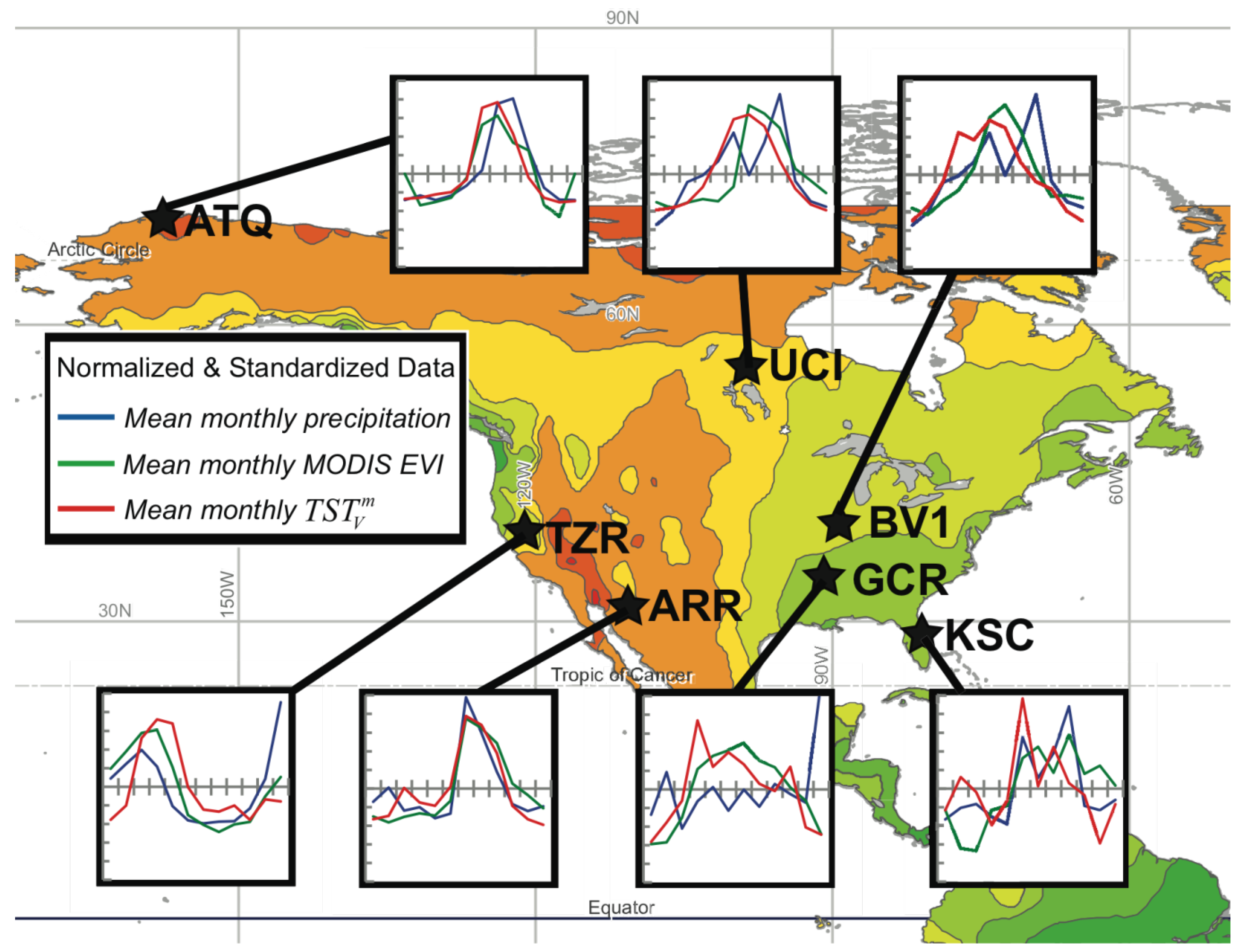
Figure 1.
The seven Fluxnet study sites used in the study, including Atqasuk (ATQ, North Slope of Alaska), Audubon Research Ranch (ARR, Arizona Semi-Arid Grassland), UCI 1964 Burn Site (UCI, Canadian Boreal Forest), Bondville Original Site (BV1, Illinois Corn & Soybeans), Goodwin Creek (GCR, Mississippi Semitropical Hardwood Forest), Kennedy Space Center Scrub-Oak (KSC, Florida Semitropical Marine Scrub), and Tonzi Ranch (TZR, Mediterranean Central California). The gradient of mean annual precipitation from wet (> 1,000 mm/yr shown in green) to dry (< 100 mm/yr shown in red) shows the diversity of climate variability captured by the selection of Fluxnet sites. The insets show the normalized (zero mean and unit standard deviation) variation of mean annual patterns of monthly precipitation, enhanced vegetation index (EVI) from MODIS, and
(see
Table 1 for a summary of climate data for each site) (vertical tick marks are 0.5 standard deviation increments above and below the mean and horizontal tick marks indicate the month of the year).
![Entropy 12 02085 g001]()
Table 1.
Climatological data and results summarized for each Fluxnet site studied.
Table 1.
Climatological data and results summarized for each Fluxnet site studied.
| Fluxnet Site | Code | Mean Annual Precipitation (mm) | Mean Annual Evapo-transpiration (ET) (mm) | Mean Annual Air Temperature θa(C) | ET Response Adaptation Factor, c | Thermal Offset Adaptation Temperature, θa (K) |
| Atqasuk | ATQ | 112 | 178 | −8 | 0.881 | 9 |
| UCI (1964 Burn Site) | UCI | 202 | 261 | 2 | 2.601 | 19 |
| Audubon Research Ranch | ARR | 389 | 290 | 17 | 1.284 | −8 |
| Tonzi Ranch | TZR | 574 | 405 | 17 | 0.805 | −9 |
| Bondville (original site) | BV1 | 839 | 603 | 11 | 0.294 | −14 |
| Kennedy Space Center (Scrub oak) | KSC | 1,120 | 808 | 22 | 0.580 | −6 |
| Goodwin Creek | GCR | 1,494 | 690 | 17 | 0.554 | −7 |
2. Methods
The methodology uses Shannon’s information Entropy [
15], which is the summation across the marginal probability function
p(x) of all discretely defined states
x of time series variable
Xt as:
We use the transfer entropy [
4]
to measure the reduction in the entropy of the current state of a measured variable
due to the knowledge of prior state τ time steps earlier in another variable
, which is in addition to the information provided by the immediate prior history of
. This is estimated using the joint and conditional probabilities as:
We use the normalized form
T` =
T / log(
m) where log(
m) is the upper bound in the estimate of entropy
for
using
m discrete bins for the estimation of the probability distribution function. We set the number of discrete states for all variables at
m = 11 defined between the lower and upper observed values of the time series variable
Xt (see [
5] for a justification for this choice
). Noting that transfer entropy is asymmetric both in strength and lag, it provides a two-way measure of information flow, or coupling strength. The
information flow process network consists of the asymmetric pair wise transfer entropy between the
ith and
jth variable from the set of
nV observed variables and can be represented as an adjacency matrix
[
5]. Process networks are computed for each of thirty-six sub-daily time lags between half an hour and eighteen hours. This range captures the primary scales of interaction between the atmospheric boundary layer (
ABL) and the terrestrial processes [
16]. Estimation and methodological issues, including robustness of the method in presence of noise, and validation using noisy chaotic data are discussed in [
5,
6].
One may choose to analyze all variables in the network
V, or a subset
S ⊆
V that characterizes a subsystem consisting of
ns variables. We use several metrics to measure flow of information [
5,
6]. The mean relative entropy for a subsystem
S ⊆
V consisting of
variables is computed as:
The mean gross information production
of a subsystem
S, is defined as:
It measures the average predictive information provided by the subsystem S to all nodes in the process networks, and therefore it is a measure of the coupling strength, or control, of the subsystem S to the rest of the system. We obtain the mean total system transport TSTmV as a special case of when S = V. An increase in TSTmV is an indicator of increased feedback between system components.
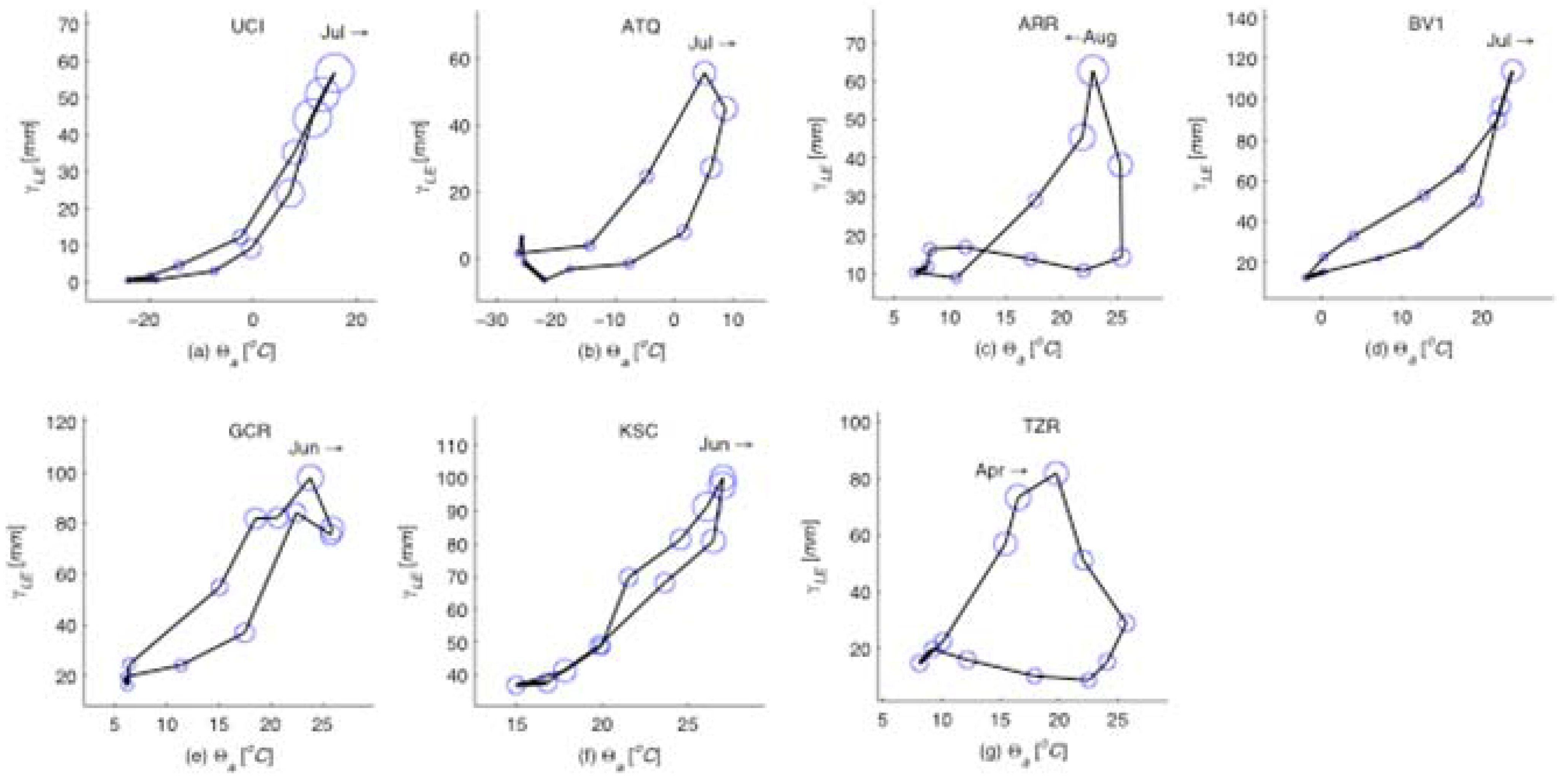
Figure 2.
Mean annual phase diagrams for for all seven sites. The size of each circle scales in proportion to , and relates ecosystem information production to the mean monthly latent heat flux (γLE) and air temperature (Θa) at each site. The month and arrow on each subplot indicate the timing of the annual peak in and the direction of chronological rotation of the phase diagram at that point (clockwise or counterclockwise). Regardless of climate and ecosystem type the peak ecosystem information production coincides with the maximum latent heat production indicating that the moisture and energy balance controlled by vegetation growth mediates the feedback between all system components.
3. Results
We find that the average information production
for the entire system
V increases linearly (not shown) along with that of the gross ecosystem productivity,
. The latter shows significant variation in the annual patterns across the different sites, and peaks during months that have relative abundance of both moisture and energy (
Figure 2). We also noticed that the information production is more strongly related to the latent heat flux than to precipitation. The seasonal patterns show interesting behavior in each of these ecohydrologic systems. For example, the Mediterranean climate at TZR site in California experiences increased information production for GEP during the spring season when latent heat is high due to the combination of increasing solar energy and available moisture from spring rains, but it plummets during the dry summer. The late summer monsoon in the Arizona desert (ARR site) results in an increase in information production following a small peak in spring and a quiet early summer. A strong midsummer peak in information production occurs in the eastern and northern ecohydrologic systems during the growing season (Alaska ATQ, Manitoba UCI, Illinois BV1), with the duration of the summer peak corresponding to the length of the growing season. By contrast, the hot and humid sites in Mississippi (GCR) and at Kennedy Space Center (KSC) experience less of a summer increase in information production since they have more steady year-round warmth and moisture.
We also found that the dependence of
on the latent heat flux
γLE and the air temperature Θ
a for all sites can be collapsed to single curves provided we account for the site specific dependencies. These take the form
(R
2=0.63,
Figure 3a) and
(R
2=0.54,
Figure 3b) where
α (=1.88 x 10
-4 mm
-1 month
-1),
β (=1.8 x 10
-7 K
-1 month
-1), and
λ (=2.78) are site independent parameters.
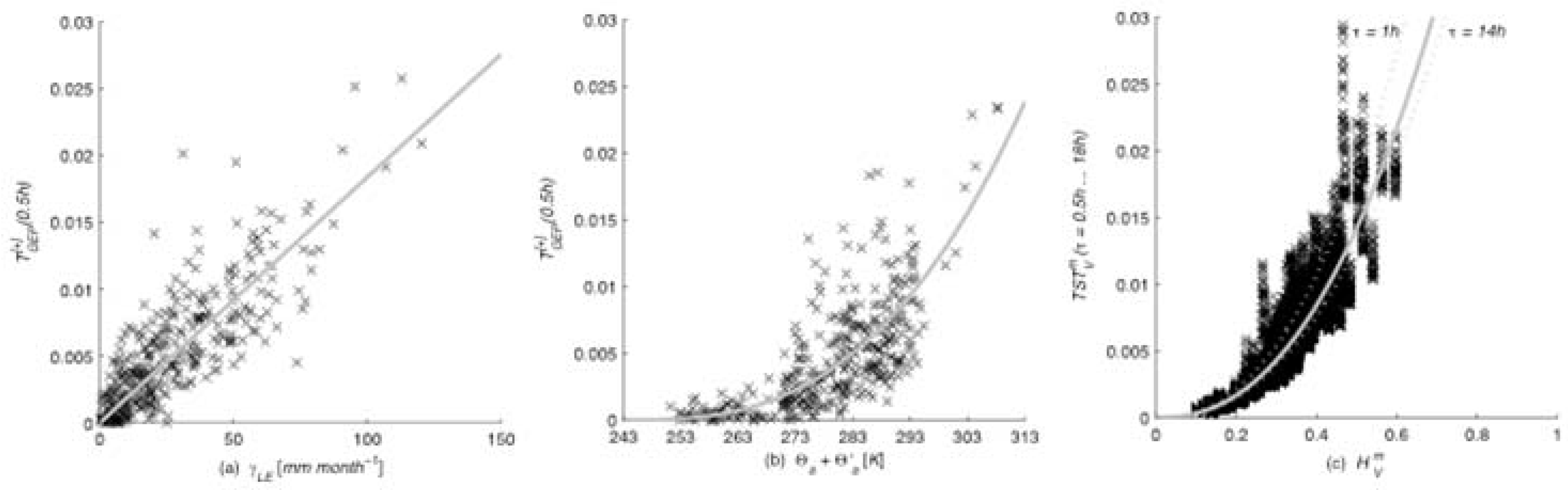
Figure 3.
For all sites information production
(a) as a function of latent heat flux follows
, and (b) as a function of air temperature follows
(see
Table 1). The whole system mean information production for all time lags
increases rapidly with increase in the entropy of the system as
(each point on the figures represents results for one month at one site and time lag).
The best-fit constant
k is empirically estimated as −243 K, where 243 K is just below the lowest recorded temperature in the dataset. The site dependent empirical constant
c and Θ
a` (
Table 1) are termed the “evapotranspiration response adaptation factor” and “thermal offset adaptation temperature.” The former captures the property that information production in humid ecosystems (eg., BV1) responds more slowly to increased moisture (lower
c) as compared to drier regions (eg., ARR), while the latter captures the behavior that ecosystems in colder regions (eg., UCI, ATQ) begin producing information at much lower temperatures (higher Θ
a`) than more temperate ecosystems (e.g., GCR, BV1). Therefore, colder and drier ecosystems are adapted to achieve higher levels of information production, that is, increased coupling, per unit of water or energy use. In other words, each ecohydrologic system is adapted to produce information,
i.e., process coupling, in a unique way, such that drier and colder systems have a more intense and immediate response to smaller amounts of moisture and energy. These results are computed using “global” bounds of variability, such that the minimum and maximum bounds on each variable
X are those of the entire long-term dataset across all sites. In this case, this means that entropies are computed relative to the full spectrum of variable states encountered over the entire observation period for the site.
The mean total system transport
increases with the average entropy of the system as
(
Figure 3c). The coefficient
a (
τ) ranges from a minimum of 0.065 at
τ =14 h, to a maximum of 0.09 at
τ =1 h (note that
is only a time step smaller than that of
) indicating that variability produces more information, that is, the system is more strongly coupled, at shorter time lags. The exponent b is 2.33 for all sites and time lags (with a standard deviation of 0.05).
Based on these observations we propose the
Information Production Hypothesis (
IPH) stated as: the feedback between system components and therefore the information production increases with increasing variability within the system. In other words, increased fluctuations in the system allow stronger coupling between system components. The system self-organizes to maximize the production of information within the bounds imposed by the entropy production of the system characterized through the functional form
, where b is found to be 2.33. This hypothesis indicates that variability is necessary for the emergence of order in complex ecohydrologic systems and that
is a universal control parameter [
17], that is, it determines the emergence of organization through feedback in the coupled system.
The IPH applies to the mean dynamics of the system as a whole involving all variables. Is the production of information also controlled by the entropy at the level of the individual variables? By focusing on specific variables or subsets within the process network, the information consumption
obtained as:
and net production
become relevant in addition to the information production
. We note that
for the whole system.
is the average predictive information received by the subsystem from all nodes in the process network. Positive
measures the extent to which the subsystem
S is controlling, as opposed to being controlled by, the rest of the network as it participates in feedback in the process network, and
vice-versa. The three metrics
,
, and
are plotted against
H`X in
Figure 4, along with the distribution of
H`X for each of the ten variables across seven sites and all months in the data.
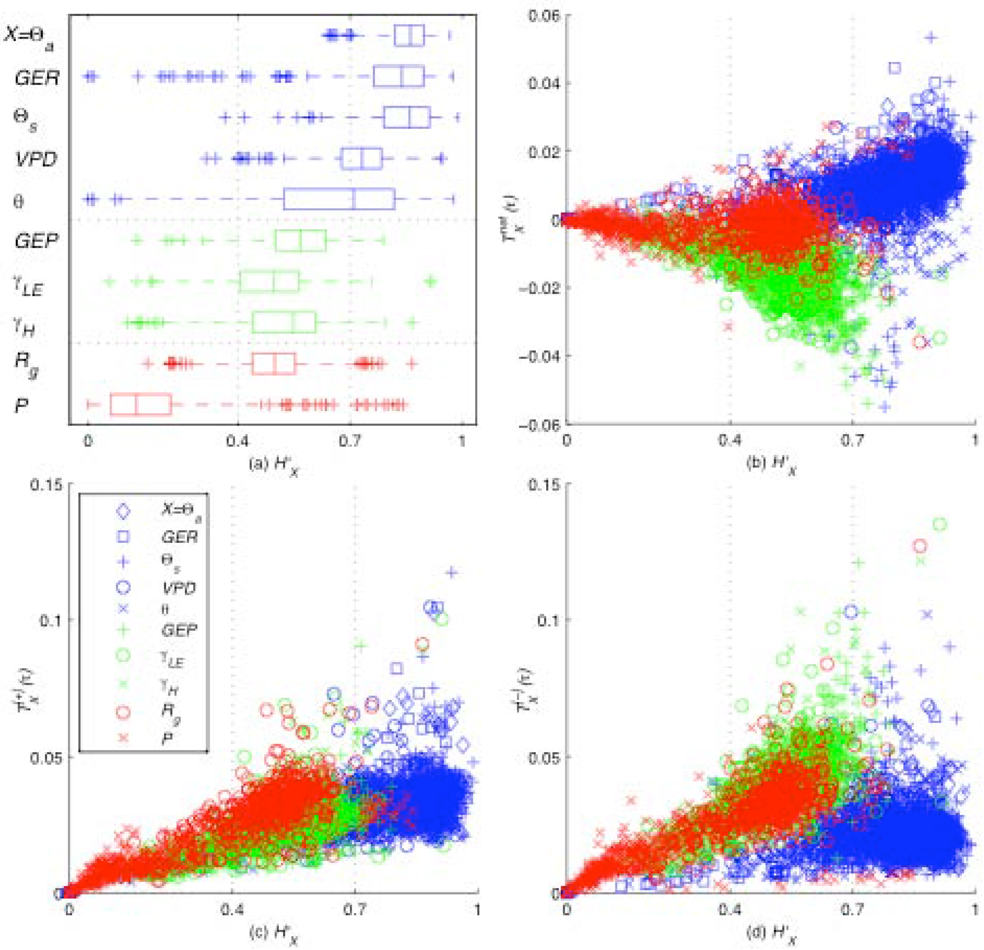
Figure 4.
Information production , consumption , and net production are plotted against each variable X’s entropy H`X, for each site, time lag, and month in this dataset. The synoptic (blue) subsystem includes weather-forcing variables, the turbulent (green) subsystem includes variables directly influenced by the ecosystem, and the ABL (red) subsystem includes precipitation and radiation. Due to an imbalance in information production and consumption as H`X increases, the net production is negative for the turbulent subsystem and is positive for the synoptic subsystem. Also observe that the smaller scale turbulent and ABL subsystems rarely take values of H`X > 0.7 but the large-scale synoptic subsystem takes values closer to the upper bound of the Shannon entropy.
We observe that information generally flows from the net-exporting “synoptic subsystem” (consisting of
Θa, GER, Θs, VPD, and
θ) to the net-importing “turbulent subsystem” (consisting of GEP,
γLE, and γH) with the “ABL subsystem” (consisting of P and
Rg) generally being net-neutral. The synoptic system varies with weather patterns on a timescale of hours to days, while turbulent systems varies with atmospheric mixing processes on a timescale of seconds to minutes, and the ABL system varies on a timescale of hours and couples the synoptic and turbulent scales [
16]. Net information flows from high-entropy larger-scale subsystems to low-entropy smaller-scale subsystems.
At the sub-daily time scales studied here, the higher entropies of the synoptic subsystem reflect the variable nature of large-scale weather patterns, and in turn, the lower entropies of the turbulent subsystem reflect the presence of stabilizing, self-organizing feedback processes between the ecosystem and its environment. The open dissipative ecohydrologic system continually consumes information from its highly variable environment to maintain their relatively self-organized state [
18]. As the net flow of information along the gradient from large to small temporal scales ebbs when water and energy become limiting so too ebbs the self-organized, information-consuming land-surface ecosystem, which exists on that gradient.
4. Discussion
By evaluating the information production, consumption, and entropy for seven climatically diverse sites, 36 independent time lags, and ten different variables (
Figure 4), it is evident that this pattern is a function of the entropy
H`X which serves as a control parameter. To explain these results, the
Moderate Entropy Hypothesis (
MEH) is proposed:
variables that participate the most in the self-organizing feedback have moderate entropy or variability (between roughly 40% and 70%, for the systems studied). The statistical results presented for the
MEH in
Figure 4 are computed using “local” bounds of variability, such that the minimum and maximum bounds on each variable
X are set independently for each local time period at each site. In this case, this means that Shannon entropies are computed relative to the full spectrum of variable states encountered over exactly one month. Therefore, while the “global” entropies allow us to capture the long-term average dynamics of the system, the “local” entropies allow us to capture the behavior of individual subsystems as they adapt to short-term variability. While the
IPH ascertains that larger variability leads to stronger feedback in the system as a whole, the
MEH indicates that increased feedback between individual components causes moderated variability in those components. This suggests a tug-of-war between the variability in the system as a whole with a tendency toward maximum variability, and the variability of individual components with a tendency toward moderate variability. This tension appears to be the causal reason for the emergence of order. Self-organizing systems evolve to maximize order (measured as information production), but this comes at the cost of increased variability (measured as entropy). Beyond relative entropy values of 70% (a rough value based on the systems studied here), it may be inferred that increased variability does not return increased order. Perhaps a further increase in the entropy of a subsystem will result in a breakdown of self-organization.
Earlier work on the use of information theory (see [
10] for a discussion) describe the ecosystems as a configuration of flows for matter and energy and the entropy provides a measure of flow diversity. Higher entropy arising from the increase in the number of configurations for flow to occur provides stability to the system under perturbation. Here in, we extend the notion of flow by considering the dynamics of information flow as a legitimate process in its own right, akin to that envisioned by [
10] with laws that are independent of and complementary to those concerning the transfer of mass, momentum, and energy. The,
IPH and
MEH govern self-organizing system dynamics originating in feedback between the system’s variables at multiple timescales. Despite the great diversity of the Earth’s climate regimes, it appears that the ecohydrologic systems are adapted to follow a simple relationship by which the system’s stochastic variability, measured as entropy, controls the emergence of order (measured as information production) across a variety of ecosystems. That is, ecosystems are adapted to their local range of variability and not the magnitude of specific control such as soil-moisture.
Further work is required to test the
IPH and
MEH and to determine their generality and use them to explain the origins of order in dynamical self-organizing systems. If the principles hold generally, they may solve an important problem by providing a mathematical basis for understanding self-organization in dynamical systems [
19]. More specifically, these hypotheses might be immediately applied to predict the evolution of ecosystems under changing and variable climate conditions. We suggest the need for work to test these hypotheses using time varying climate data to examine the system’s behavior at larger and smaller spatio-temporal scales, and the dynamics of synthetic complex systems (e.g., systems examined by [
20,
21,
22]).


