
Simple Methods for Improving the Forensic Classification between Computer-Graphics Images and Natural Images

Univ. Grenoble Alpes, CNRS, Grenoble INP, GIPSA-Lab, 38000 Grenoble, France
*
Author to whom correspondence should be addressed.
Forensic Sci. 2024, 4(1), 164-183; https://doi.org/10.3390/forensicsci4010010
Submission received: 23 January 2024
/
Revised: 26 February 2024
/
Accepted: 12 March 2024
/
Published: 14 March 2024
Abstract
:From the information forensics point of view, it is important to correctly classify between natural images (outputs of digital cameras) and computer-graphics images (outputs of advanced graphics rendering engines), so as to know the source of the images and the authenticity of the scenes described in the images. It is challenging to achieve good classification performance when the forensic classifier is tested on computer-graphics images generated by unknown rendering engines and when we have a limited number of training samples. In this paper, we propose two simple yet effective methods to improve the classification performance under such challenging situations, respectively based on data augmentation and the combination of local and global prediction results. Compared with existing methods, our methods are conceptually simple and computationally efficient, while achieving satisfying classification accuracy. Experimental results on datasets comprising computer-graphics images generated by four popular and advanced graphics rendering engines demonstrate the effectiveness of the proposed methods.
1. Introduction
The recent development of easy-to-access and highly efficient image-generation and -modification tools has made it easy to obtain high-quality synthetic and manipulated images, which would create a safety concern about the authenticity of digital images. Accordingly, this has given rise to the rapid development of the research on image forensics [1,2] whose aim is to detect and analyze the source of images or the possible modifications made to images. In this paper, we consider and study a specific image forensic problem, that is, the classification between natural images (NIs) that are acquired by digital cameras and computer-graphics (CG) images that are generated by advanced graphics rendering engines. From an information forensics point of view, NIs describe what has happened in the real world, while CG images depict fictive scenes. Therefore, it is important to correctly classify between NIs and CG images, so as to faithfully determine the source of images and the authenticity of the scenes described in the images. More specifically, as CG images reach a level of photorealism that makes them in many cases indistinguishable to human naked eyes from NIs (Figure 1 shows some examples), it has become necessary to develop reliable forensic methods for detecting these synthetic CG images [3,4]. Hereafter and following [5], we call this specific image forensic problem the CG forensics problem.
The main objective of our work is to improve the forensic classification of NIs and CG images in two challenging situations, i.e., when a trained forensic classifier is tested on CG images created by rendering engines that remain unknown during the training phase or when we have a limited number of training samples. For the first situation, in an existing state-of-the-art method [5], the classification performance on CG images from unknown rendering engines, i.e., the so-called generalization performance, is improved by carrying out an additional enhanced training procedure with specifically created supplementary and artificial samples. This method can be effective in improving the generalization capability, but the additional enhanced training procedure remains computationally costly and complicated. In this paper, we instead propose simple methods, based on data augmentation and the combination of local and global prediction results, to boost the generalization performance. Our methods are conceptually simple and computationally efficient compared to the existing method, while achieving satisfying classification performance. For the second situation of sample scarcity, to the best of our knowledge, we conduct in this paper the first comprehensive experimental study in the literature on testing and improving the forensic performance when we have a limited number of training samples. We show that our simple methods mentioned above are also able to improve the forensic classification accuracy between NIs and CG images in this challenging yet very practical situation.
Our contributions are summarized as follows:
- We have investigated a simple yet effective method of carefully designed data-augmentation operations to improve the forensic classification performance between NIs and CG images;
- We have studied the combination of local and global prediction results in order to determine the loss function of a neural network and thus to make better use of the information contained in each image for achieving better classification results for the CG forensics problem;
- We have carried out experimental studies to test and validate the above two methods, which achieved an improvement in terms of the generalization capability and the test accuracy with reduced training sets, while remaining computationally efficient.
The remainder of this paper is organized as follows. In Section 2, we provide a brief overview of the related work in the CG forensics research. We introduce in Section 3 the datasets and neural network used in our study. Section 4 presents the motivations and the technical details of our proposed methods. In Section 5, we report and analyze the experimental results. Finally, we draw conclusions and discuss possible future improvements in Section 6.
2. Related Work
The traditional methods proposed for the classification of CG images and NIs were based on the manual construction of carefully designed discriminative features. These features could be extracted from either the spatial image data [11,12,13] or from a frequency-like transformed domain [3,14,15]. The images’ spatial properties considered for the extraction of discriminative features include texture details, geometric features, the color distribution, edge statistics, a combination of such properties, etc. Transforming the image from the spatial domain to a frequency-like domain has the potential to reveal features that are not visually apparent in the image but that are discriminative to distinguish CG images from NIs. For example, Lyu and Farid [3] combined the wavelet statistics of the first four orders (i.e., mean, variance, skewness and kurtosis) as the feature to discriminate between NIs and CG images.
While these hand-made features are easy to understand and explain, they are also complicated to design, and the performance of feature-based detection remains experimentally inferior to that of recent deep learning-based methods. Indeed, since the development of the AlexNet neural network [16], deep learning [17] has demonstrated its superiority for almost all image-processing and -analysis tasks, including image forensic analysis. While the traditional methods work in two stages, a first stage of feature extraction and a second stage of classification based on the extracted features, neural networks combine these two stages and work as a whole in an end-to-end process. Due to their high learning capacity, neural networks are able to automatically extract discriminative features that distinguish CG images from NIs well, thus avoiding the time-consuming feature-design stage. In general, recent deep learning-based methods [4,5,10,18,19], leveraging various neural network architectures, deliver better forensic results than the traditional methods.
Very few existing works considered the two challenging yet practical situations mentioned in Section 1, i.e., the generalization capability on CG images created by unknown rendering engines and the forensic performance in the case of training data scarcity. To the best of our knowledge, the only dedicated research work on improving the generalization capability was conducted by Quan et al. [5], who proposed to construct harder artificial samples and to carry out an additional enhanced training procedure by using these supplementary artificial samples. The generalization performance was improved with a relatively high additional computational cost of the network training, because the enhanced training in general lasts several hours on an advanced GPU (graphics processing unit). In this paper, we propose much simpler and computationally much more efficient methods, which in the meanwhile achieve a comparable or even slightly better generalization performance when compared to the state-of-the-art method proposed in [5]. The data-scarcity situation was partially considered in our recent paper [10] by leveraging self-supervised pre-training, though with a very limited experimental setting. One drawback of the method of [10] is the high computational cost of the self-supervised pre-training procedure, with more than ten hours of parallel computation on two advanced GPUs. In this paper, to our knowledge, we conduct and present a first comprehensive study in the literature on the CG forensics problem in the case of training-data scarcity, by considering different numbers of available training samples with CG images generated respectively by four popular graphics rendering engines. In this data-scarcity situation, by using our computationally efficient methods, we are able to obtain good forensic performances on CG images generated by both known and unknown rendering engines.
3. Datasets and Network
Before presenting our proposed methods in the next section, in the following we introduce the datasets (Section 3.1) and the backbone neural network (Section 3.2) utilized in our study.
3.1. Datasets
The selected data for training and testing are crucial. In our study, we use the datasets collected and shared by Quan et al. [5] because of the high visual quality and diversity of the CG images included in the datasets. The datasets of [5] contain both CG images and NIs, and the CG images are from four different rendering tools, which makes the datasets very suitable for experimental studies on the evaluation of generalization performance. More specifically, the CG images in the datasets were generated by the advanced graphics rendering tools of Artlantis [20], Autodesk [21], Corona [7] and VRay [6], all chosen for their very high degree of photorealism. It is difficult to know the exact techniques utilized in these rendering engines because they are commercial products with restrictions. These tools may share some common points, e.g., they are probably based on the effective solving of the fundamental rendering equation and/or the concept of ray tracing, but differences should exist for example in terms of technical details when handling light–material interactions, light diffraction, shading, shadows, etc. This can result in a rather limited generalization performance across CG images produced by different rendering engines. The CG images in the datasets of [5] were downloaded from the respective websites of the four rendering tools. The numbers of CG images from Artlantis, Autodesk, Corona and VRay tools are 1620, 1620, 1593 and 1579, respectively. For each dataset corresponding to a rendering tool, 360 CG images were randomly selected to form the test set, and the remaining CG images were retained for the training set.
To maintain the diversity of natural images, NIs from two popular existing databases, i.e., RAISE [9] and VISION [8], were combined. Out of the 8156 high-resolution images contained in the RAISE database, 4700 were randomly selected. In order to simulate real-world conditions, these images were randomly resized and compressed (details in [5]). The VISION database comprises images captured by 35 mobile devices, with each device contributing 100 NIs, and in total VISION has 3500 NIs. Additionally, these natural images were exchanged via Facebook (in high and low quality) and WhatsApp, resulting in four versions for each image [8]. A random selection was made from these four versions for each image to maintain the total number of 3500 selected NIs. We note that the CG images as downloaded from the websites of the four rendering tools are of different spatial sizes and different compression qualities. By contrast, the NIs from RAISE [9] are never-compressed, high-resolution images, and the NIs from VISION [8] (before being exchanged via Facebook and WhatsApp) are of limited size and compression settings. Therefore, it is reasonable to randomly resize and compress NIs from RAISE (following the same procedure as suggested in [5]) and to exchange NIs from VISION via social network platforms (as carried out by the original authors of VISION [8]). This would allow us to obtain CG images and NIs that are overall quite comparable in terms of their spatial size and compression quality.
In the end, 8200 natural images were selected from RAISE and VISION, with 4700 from RAISE and 3500 from VISION. Quan et al. [5] randomly chose 5040 NIs and duplicated each CG image in a training set approximately four times to obtain 5040 CG images to be included in the training set. In this way, four training sets, balanced between NIs and CG images, were constructed, corresponding to the four graphics rendering tools. Each training set comprises 10,080 images, i.e., 5040 CG images from a specific rendering tool and 5040 NIs. In addition, 360 natural images were selected from the remaining NIs and combined with corresponding CG images to constitute four test sets, each including 360 NIs and 360 CG images from a specific rendering engine. For the sake of simplicity and with a little abuse of the names, we hereafter use Artlantis, Autodesk, Corona and VRay to name the four datasets, each comprising balanced (i.e., with an equal number of NIs and CG images) training and test sets. Examples of CG images and NIs are illustrated in Figure 1.
- Reduced datasets. In addition to conducting an experimental study on the full datasets detailed above, we aimed to carry out a comprehensive study of the forensic performance on reduced datasets, corresponding to the challenging situation with training data scarcity. Reducing the amount of data for training brings us closer to real-life application conditions, where obtaining large quantities of data is often complicated. In order to prepare experimental data for this challenging yet practical situation, we constructed different versions of reduced datasets from the full datasets of [5], with different ratios of images from the full datasets. More specifically, for each full training set with 10,080 images, we used four reduction ratios of 50%, 20%, 10% and 5% to construct reduced training sets with respectively 5040, 2016, 1008 and 504 images. For each ratio, we still had four training sets corresponding to the four rendering engines, and all the reduced training sets still remained balanced with an equal number of CG images and NIs. The test sets remained unchanged when the training was carried out on reduced or full training sets, so that we could fairly evaluate and compare the test classification performance under different qualities of training samples. We report experimental results on both full and reduced datasets in Section 5.
3.2. Neural Network
We base our study on the ENet neural network developed in [5], because it reached state-of-the-art performance on the full datasets described above. ENet is a neural network with ten layers and two branches at the beginning that takes the NcgNet [4] architecture as the base network. It is designed to focus on learning diverse features. It has the purpose to automatically combine kernel initialization with SRM (spatial rich model) [22] filters and the conventional Gaussian random initialization in the beginning of the network. This combination is useful for learning discriminative and diverse features for the CG forensics problem. The architecture of ENet is illustrated in Figure 2. The first part, spanning from layers L1 to L4 in Figure 2, features a novel two-branch design, while subsequent layers maintain the NcgNet architecture. The input to ENet is an RGB image.
4. Proposed Methods
In this section, we first explain the reasons and motivations that have led us to adopt our research ideas to improve the forensic classification performance between NIs and CG images (Section 4.1). Then, we propose and describe simple methods, based on suitable data-augmentation operations (Section 4.2) and a slight modification of the network architecture and loss function (Section 4.3), to achieve effective discrimination between NIs and CG images, especially when the forensic classifier is tested on CG images created by unknown graphics rendering engines and/or when we have a limited number of training samples.
4.1. Motivations
The existing studies in [5,10] show that methods based on additional enhanced training or self-supervised pre-training can be used to improve forensic classification capabilities in some challenging situations. However, those methods are expensive in terms of computational cost, with several hours [5] or more than a dozen of hours [10] of extra training time. For this reason, in this paper we investigate simple and efficient methods based on data augmentation and the combination of local and global predictions, as these methods are much less expensive in terms of computational cost. As shown later in the experimental studies in Section 5, the extra computation time induced by our methods is around 10 to 20 min, which is much less than the existing methods. As far as the data-augmentation method is concerned, two categories of augmentation operations will be studied. The first category consists in reducing the impact of subtle differences potentially related to the processing history of the images that often reside in the high-frequency components. The purpose is to encourage the neural network to learn discriminative and generalizable features to distinguish between NIs and CG images, but not features that may pertain to the minor differences in terms of the image processing history. The second category of data-augmentation operations consists in increasing the diversity of the training data, in order to enable the neural network to improve its ability to generalize and to decrease the risk of overfitting. Lastly, the combination of local and global predictions encourages the consistency of classification results over the whole image, and this would be beneficial to obtain comprehensive features focusing not only on globally prominent clues but also on diverse local clues for the forensic classification. With the proposed methods that promote the better quality of the learned features, experimentally we are able to achieve better forensic classification results when the classifier is trained and/or tested on the challenging situations mentioned previously.
4.2. Data Augmentation
Data augmentation refers to methods used to produce new data from the basic training data available for a machine learning problem. The produced new training data, if well constructed, are likely to improve the learning therefore the performance of machine learning algorithms. Data augmentation has received relatively little attention in the research on CG forensics. Existing methods tend to use simple augmentation operations like random cropping and horizontal flipping [4,5]. In this paper, we would like to carefully study the effect of two categories of data-augmentation operations (as detailed later in this subsection) on the forensic performance of the classification between NIs and CG images.
4.2.1. Reducing the Impact of Processing History
As mentioned above, the data-augmentation operations we consider can be divided into two categories. By applying the first category of operations, our objective is to reduce the impact of the processing history traces of images on the training of neural network. These subtle yet minor traces generally reside in the high-frequency components of training images and they would not reflect the intrinsic difference between NIs and CG images. Intuitively, it would be beneficial to reduce the impact of such traces on our forensic classification problem and to somewhat homogenize these traces for the NIs and CG images used for training. This would make it more difficult to distinguish between them, and encourage the neural network to focus on features that truly reflect the natural (NI) or synthetic (CG) nature of the images.
In order to reduce the impact of such minor and high-frequency traces, we propose to apply two data-augmentation operations of somewhat opposite ideas. The first operation consists in random noise addition, in an attempt to “cover” existing traces by introducing new and “consistent” high-frequency traces with the added noise. The second operation, by contrast, consists in removing part of the existing traces via the augmentation operation of Gaussian blurring. Gaussian blurring is a classical and popular image-processing method. In our work, it enables us to attenuate the high-frequency elements in images where traces of the image-processing history may reside. Technically and more precisely, for a given training image, we apply, with a 50% probability, a convolution operation by using a kernel constructed with the following Gaussian function:
where x and y represent the distance on the x-axis and the y-axis, respectively, from the kernel center. We apply this Gaussian blur augmentation with a value (which corresponds to the standard deviation of the Gaussian function above) randomly drawn between and 2, and with a kernel of the size . Figure 3 shows an example of an image before and after applying Gaussian blurring. Experimentally, we found that the Gaussian blur augmentation leads to better forensic performances than the noise-addition augmentation. The results and analysis are provided in Section 5.
4.2.2. Increasing the Diversity of Training Samples
The second category of data augmentation consists in enriching the diversity of the images used for training, in order to obtain a trained network with a better generalization capacity. The underlying idea is to have more diverse training samples by introducing reasonable modifications to the available training images. Operations such as color jitter and color transfer between images fall into this second category.
The color jitter operation brings random modification to the color-metric properties of a given training image. In practice, random perturbations can be introduced to the brightness, contrast, saturation and hue of the image, so as to have more diverse training samples. Another advanced and alternative augmentation operation is the color transfer between two images. Our implementation of this operation is based on the landmark work of Reinhard et al. [23], in which the authors proposed a method for transferring low-order color properties from a source image to a target image. The color transfer is realized in the color space, which achieves better transfer performance than the conventional RGB space, as shown in the original paper [23]. More precisely, first- and second-order statistics of the means and standard deviations of the channels are considered and transferred. In our study, within a balanced batch (i.e., an equal number of NIs and CG images) fed to the neural network, we randomly pair NIs and CG images and then transfer, for randomly selected 50% pairs, the color of the NI in a selected pair to the CG image in the pair. In this way, the CG images used for training can have more diverse and also more realistic (because of the color transferred from an NI) color properties. This is beneficial to achieving a better forensic performance in the challenging situations considered in this paper. An example of the result of this color transfer operation is shown in Figure 4, and the adopted color-transfer algorithm is summarized in Algorithm 1.
| Algorithm 1 Color transfer from a source image to a target image. |
|
It is worthwhile pointing out that these two operations of data augmentation, i.e., color jitter and color transfer, both aim to increase data diversity but differ in the way they do so. The color jitter operation augments the data in a rather random way, whereas the color transfer operation consists in transferring statistical color properties from a natural image to the virtual scene of a CG image. As far as we know, it is new in the literature of image forensics research to make use of data augmentation based on color transfer for improving the forensic performance. Experimentally, both color jitter and color transfer in general can improve the CG forensics performances. In addition, we can gain further improvement with the combination of color jitter or color transfer with the Gaussian blurring operation from the first category. Detailed experimental results are presented in Section 5.
4.3. Combining Local and Global Predictions
Another method aimed at improving the results obtained by our trained network is to slightly modify its architecture in order to encourage it not only to predict a global binary result over an entire image (i.e., an NI or CG image), but also to produce different local prediction results, calculated from sub-divisions of the image. This is reasonable because local parts of an NI or CG image still remain natural or computer-graphics sub-images, without changing their forensic labels (NI or CG). The intuition and objective of combining local and global prediction results is to encourage the network to not only focus on globally prominent features for the forensic classification, but also to carefully check local sub-parts of the image to hopefully derive comprehensive features that would still be useful in the challenging forensic situations considered in this paper. More precisely and as illustrated in Figure 5, at the output of the convolutional layer L7, we add a new branch where the output feature maps of L7 are divided into P sub-parts of equal size (here as shown in Figure 5 and in our implementation there are sub-parts). We add a new FC layer (denoted by FC_local) with a proper dimension to cope with the new input of a sub-part of feature maps to further analyze the sub-part. In the other branch, the whole output feature maps of L7 are analyzed with the FC layer at L8 (denoted by FC_global) as in the original ENet. Afterwards, the output of FC_global, as well as the P outputs of FC_local, are separately input to the remaining part of the network for further analysis by the FC layers at L9 and L10. Therefore, finally we have classification scores at the outputs of the final L10 layer.
Accordingly, we modify the loss function so that it takes into account both the global and the local predictions. In our implementation, the final loss for the training of the modified network is the sum of the global prediction loss and the average of the P local prediction losses. More precisely, the global prediction loss is calculated as the conventional cross-entropy loss as follows:
where is an input, is the target label of , c represents the class index (here for a binary classification problem we have or respectively representing the NI or CG image classes), is the raw classification score of the sample being classified as of class c, and N represents the number of training samples.
With a little abuse of notation, we can equivalently consider that the local loss is computed on a sub-part of a training sample. Therefore, similar to the computation of the global prediction loss presented above, the local loss for a sub-part of sample with the sub-part index i () is computed as follows:
Finally, the final loss function of the modified network considering both local and global predictions is calculated as follows:
Experimental results of this modified network trained with the modified loss taking into account both local and global predictions are presented in the next section. The obtained results show the effectiveness of this new training strategy, especially when combined with the data-augmentation operations presented in Section 4.2 and when there are very few available training samples.
5. Experimental Results
Our methods were implemented by using PyTorch and tested on the datasets described in Section 3.1. In the following, we present experimental results obtained on both full and reduced datasets as well as some comparisons.
5.1. Results on Full Datasets
We first carried out experiments on the full datasets. As mentioned in Section 3.1, there are four full datasets, with CG images created respectively by the four advanced rendering engines Artlantis, Autodesk, Corona and VRay. We tested the forensic performance of the neural network of various variants with data augmentation and/or modified loss function, when it was trained on each of the four datasets. For each trained network on a specific dataset (e.g., the training set of Autodesk), we tested and report its classification accuracy on the four test sets, with CG images from the known rendering engine during the training phase (e.g., in this case the test set of Autodesk), as well as from the other three unknown rendering engines (e.g., in this case the test sets of Artlantis, Corona and VRay). In this and the following subsections, we consider the average test accuracy on the four test sets as the main performance metric, because it reflects both the conventional classification accuracy on the known rendering engine and the generalization performances on the unknown rendering engines. We also provide, in some cases, the detained accuracy results on individual test sets.
We present in Table 1, Table 2, Table 3 and Table 4 the results obtained respectively when we trained the network on the four full datasets of Artlantis, Autodesk, Corona and VRay. We report the test classification accuracy, individual ones and the average on the test sets. The generalization performances on test sets with CG images from unknown rendering engines are shown in italic in the tables. We present the results of normal training (the same as the baseline method in [5]), training with noise addition (NA) augmentation, with Gaussian blurring (GB) augmentation, with color jitter (CJ) augmentation, with color transfer (CT) augmentation, with the modified new loss taking into account both global and local predictions, with the augmentation of GB + CJ, with the augmentation of GB + CT and with the combination of the modified new loss and the augmentation of GB + CT.
We have several observations regarding the results presented in Table 1, Table 2, Table 3 and Table 4. For the first category of augmentation operations, Gaussian blurring (GB) worked much better than noise addition (NA), with much higher average classification accuracies in the last column of all four tables. GB consistently improved the average accuracy on all four datasets when compared to the baseline normal training of [5], while NA could only cause improvement when trained on Corona. This may imply that in order to reduce the impact of the processing history of training images, smoothing (i.e., partially removing high-frequency components) is a much more effective way than noise addition (i.e., introducing new high-frequency components in an attempt to “cover” old ones). For the second category of augmentation, both color jitter (CJ) and color transfer (CT) improved the average test accuracy on the four datasets compared to normal training, except for CJ with training on the VRay dataset (Table 4). However, whereas CJ improved the average test accuracies in Table 1, Table 2 and Table 3, CJ offered bigger improvements of the forensic performance than CT. The modified new loss with a slightly modified network architecture led to a higher average test accuracy than the normal training when trained on Autodesk, Corona and VRay, but it decreased the accuracy when trained on Artlantis. As presented and analyzed later in this section, when the new loss was combined with data-augmentation operations, we achieved a consistent improvement of the forensic performance and in many cases a considerable boost of the test accuracy, especially in the challenging situation of training data scarcity as considered and studied in the next subsection.
We also have in Table 1, Table 2, Table 3 and Table 4 interesting results and observations regarding the combination of several methods, as listed in the last three rows of these four tables. First, when we combine the two categories of augmentation operations, we find that the combination of GB + CT works consistently better than the combination of GB + CJ. This is quite interesting, because CJ alone can work better than CT (when trained on Artlantis, Autodesk and Corona, but not on VRay). One possible explanation is that CJ, which introduces random perturbations to images, may somewhat enhance the processing history traces that GB aims to partially remove; therefore, the combination of GB + CJ might weaken the effect of the individual augmentation operation of GB or CJ. By contrast, the combination of GB + CT reached the highest average test accuracy among all methods when trained on Artlantis, Autodesk and Corona, i.e., as shown by the average test accuracy values in bold in the last column of Table 1, Table 2 and Table 3. More precisely, this combined augmentation of GB + CT improved the average test accuracy from , and for normal training [5], respectively when trained on Artlantis, Autodesk and Corona, to , and . It appears that with this combination, both GB and CT can achieve their respective objective of reducing the impact of the processing history and increasing the diversity of training samples, without interfering with each other. Finally, the combination of modified loss, GB and CT also provides consistently good results in the four tables, in particular achieving the highest average test accuracy of when trained on VRay, as shown in Table 4. As presented in the next subsection, we will see that this combination of modified loss + GB + CT shows its big advantage and outperforms other methods in the challenging situation where we have very few training samples.
5.2. Results on Reduced Datasets
We also conducted experiments on reduced datasets. As mentioned at the end of Section 3.1, we used four reduction ratios, i.e., 50%, 20%, 10% and 5%, to construct four versions of reduced datasets. It is worthwhile pointing out that for each reduction ratio, we still have four reduced datasets corresponding to the four rendering engines Artlantis, Autodesk, Corona and VRay. The average test accuracy on all four test sets, as defined in Section 5.1, is again used as the main performance evaluation metric, which considers the test accuracy for both known and unknown rendering engines.
We first of all verified that the reduction of the number of training samples indeed led to a decrease in forensic performance. To this end, we show in Figure 6 the comparison between the average test accuracy of classifiers with normal training [5] on the full dataset and the reduced datasets of four different ratios, when trained on the training set of Artlantis, Autodesk, Corona and VRay. It can be observed that in general, the average test accuracy decreased as the reduction ratio increased; there are two minor exceptions (the Artlantis 5% reduced dataset and Corona 50% reduced dataset), which in our opinion are mainly due to the randomness of the neural network initialization and training procedure. It can be noticed from Figure 6 that when we have very little training data, say 5% of the full training set, the average test accuracy can be as low as around , as shown by the purple bars in the figure.
We present in Table 5, Table 6, Table 7 and Table 8 the results of the average test accuracy of the different methods when they were trained on reduced training sets of Artlantis, Autodesk, Corona and VRay. In each table, we show the results under different reduction ratios of the training set (i.e., 50%, 20%, 10% and 5%), and we also provide the corresponding results obtained with full training sets for easy comparisons.
We have some interesting observations from these tables. First, with the reduced training sets, the individual methods, i.e., with GB augmentation, with CJ augmentation, with CT augmentation and with the modified new loss, were effective in improving the forensic performance compared to the normal training in a majority of cases. Second, with the combination of several methods, i.e., with augmentation of GB + CT and with the combination of the new loss and the augmentation of GB + CT (last two rows in Table 5, Table 6, Table 7 and Table 8), a consistent improvement was achieved in every column of these tables when compared to normal training, as well as the best average test accuracy in almost every test scenario, as highlighted by the value in bold in each column of Table 5, Table 6, Table 7 and Table 8. Finally, if we take a close look at the results with different reduction ratios, we can observe that for moderate reduction ratios of 50% and 20%, the augmentation of GB + CT (second-last row) and the combination of the new loss and the augmentation of GB + CT (last row) have rather comparable overall results in the four tables, while it is clear that the combination of the new loss and the augmentation of GB + CT (last row) has the highest average test accuracy for very aggressive reduction ratios of 10% and 5% in the last two columns of the four tables. More precisely, this combination of new loss + GB + CT achieved an improvement of as high as (from to ) compared to normal training on the reduced Corona training set of 10% (second-last column of Table 7), and a considerable improvement of (from to ) for the reduced VRay training set of 5% (last column of Table 8).
In our experiments, we have also noticed that for the reduced training set of the extremely low reduction ratio of 5%, the method of the combination of the modified new loss and the augmentation of GB + CT always led to an improvement of test accuracy in all test cases on an individual test set. In total, there are 16 test cases, i.e., we have 4 reduced (5% ratio) training sets of Artlantis, Autodesk, Corona and VRay and for each reduced training set we have 4 test sets corresponding to the four rendering engines. For the sake of brevity, in Figure 7 we show, as an example, the obtained improvement compared to the normal training when trained on the reduced (5% ratio) training set of Artlantis. Concretely, with the combination of new loss + GB + CT, we achieved a considerable improvement in terms of the conventional test accuracy with the known rendering engine Artlantis (from to , the first group of bars in the figure), as well as the generalization performances on unknown rendering engines of Autodesk, Corona and VRay (respectively from to , from to , and from to , the last three groups of bars in the figure). We mention in this paragraph and show in Figure 7 the detailed results on individual test sets to showcase the striking performance improvement when we have an extremely low number of training samples with a very low reduction ratio of 5%. Our method also showed good performances for other reduction ratios; for example, with the 10% reduction ratio, the combination of the modified new loss and the augmentation of GB + CT could improve the classification accuracy on 14 out of all 16 individual test cases, with a significant improvement in terms of the average test accuracy, as shown in the second-last column of Table 5, Table 6, Table 7 and Table 8. For the sake of brevity (all results of the main evaluation metric of the average test accuracy are provided in Table 5, Table 6, Table 7 and Table 8 for all reduced datasets), we refrain from presenting detailed results for every reduction ratio.
5.3. Comparisons in Terms of Test Accuracy and Training Time
We now compare our methods with two state-of-the-art methods [5,10] that also consider the challenging situations of generalization performances and training data scarcity. Comparisons are carried out in terms of the test accuracy and training computational cost.
We first compare with the method of Quan et al. [5], who proposed to improve the generalization performance by carrying out an additional enhanced training procedure. Table 9 compares the training computational cost of the enhanced training method in [5] and the different variants of our method when trained on the full Artlantis training set. All the experiments were carried out on the same NVIDIA RTX A6000 GPU. We can see from Table 9 that our different methods result in a slight increase of around 10 or 20 min of training time, when compared to the baseline normal training (also from Quan et al. [5]). The additional training time is slightly lower than 10 min for the augmentation methods and the proposed modified network architecture and loss function. The combination of data augmentation and the modified new loss leads to an increase in training time of about 20 min. This remains acceptable and seems to confirm that our methods provide a real improvement in forensic performance without inducing an excessive increase in the computation time of network training. By contrast, the enhanced training proposed in [5] led to an additional training time of more than 5 h, which is significantly more costly than our methods. It is important to note that our focus in this paper is on reducing the computational cost of the training phase, which lasts a much longer time and thus has a much higher energy consumption footprint when compared to the test (inference) phase. Our proposed methods have practically no impact on the inference time during the testing phase. More precisely, for all trained networks of different variants, i.e., with normal training, with additional enhanced training [5], our various data-augmentation operations, and our new loss or combination of our proposed methods, the inference time on each test image is about 23 milliseconds. This ensures a high test speed with about 43 test images processed every second. Table 10 presents a comparison of the test accuracy results between the enhanced training method of [5] and our method of the combination of the augmentation of GB + CT, when trained on the four full datasets. We limit the comparison to the full datasets because the method in [5] only considered these full datasets, and the extension to reduced datasets remains quite complicated because some key parameters need to be properly adjusted. In Table 10, the results are presented in pairs of test accuracy values separated by a slash sign “/”, with the former being the result of [5] and the latter the result of our method. It can be observed from Table 10 that our method has comparable or even slightly better forensic test performance than the state-of-the-art method of [5], with consistently higher average test accuracies for all four experimental scenarios. In addition, it is worthwhile mentioning that our method achieves this level of performance with much less training computational cost compared to the enhanced training method of [5], as shown by the results in Table 9.
We then carried out comparisons with our recent method in [10], which partially considered the situation of training data scarcity though with a quite limited experimental setting. Table 11 presents a comparison of test accuracy results between the method of [10] and our method of the combination of new loss + GB + CT, when trained on reduced training sets with a reduction ratio of 20% (this is the only data scarcity setting considered in [10], with a self-supervised pre-training and then a fine-tuning on the reduced training set). Results are still presented in pairs with a slash sign separating the result of [10] and that of our method. The results in Table 11 show that our method achieves an improvement of the test accuracy when compared with [10] in the vast majority of individual test cases. In addition, the average test accuracy of our method is higher that that of [10] for all four reduced training sets (last column of Table 11), with an improvement of at least (trained on 20% VRay) and of at most (trained on 20% Artlantis). This better forensic performance is achieved by our method with much less training computational cost than the method of [10]. Our method only needs an additional training time of about 20 min compared to normal training on a single GPU of NVIDIA RTX A6000, while the method of [10] required a self-supervised pre-training that lasted as long as 14 h with parallel computation on two GPUs (one NVIDIA RTX A6000 and one NVIDIA Quadro P6000).
5.4. Discussion
From the experimental results presented above we can see that our proposed methods of data augmentation and the modified new loss function, when applied separately, are able to improve the performance for the CG forensics problem in many test scenarios. When we combine these methods of different categories, better forensic performances can be achieved. In particular, by using the combination of the modified new loss and the augmentation operations of Gaussian blurring (GB) and color transfer (CT), we can safely obtain the highest average test accuracy in the challenging situations with very few training samples, i.e., with the reduction ratios of 10% and 5% of the training sets as shown in the last two columns of Table 5, Table 6, Table 7 and Table 8. On the full datasets, both the augmentation of GB + CT and the combination of the new loss + GB + CT can consistently improve the average test accuracy when compared to the baseline normal training (cf. the results in the second column of Table 5, Table 6, Table 7 and Table 8), with the former achieving slightly better overall performance. It appears that our proposed methods, which are designed to realize different objectives (i.e., reducing the impact of the data processing history, increasing the data diversity and learning comprehensive features with the combination of local and global predictions), can be complementary to each other. In addition, our methods are conceptually simple and computationally efficient, as shown by the comparison results with existing methods. Our proposed methods induce an additional training time of about 10 to 20 min, while the existing methods, based on enhanced training or self-supervised pre-training, require respectively more than 5 h or 14 h of additional computation time of training.
6. Conclusions and Future Work
In this paper, we carried out studies to improve the forensic performance for distinguishing between NIs and CG images, in the challenging situations of tests on CG images produced by unknown rendering engines and of training data scarcity. Differently from existing methods that remain computational costly for the training phase, we proposed to leverage efficient yet effective solutions of appropriate augmentation operations and of slightly modified network architecture and loss function, with the objective to learn more useful features to cope with the considered challenging situations. A series of experiments were conducted on datasets comprising CG images created by four advanced graphics rendering engines. The experimental results demonstrate the utility of our proposed methods in improving the forensic performance, especially the generalization capability and the classification performance when there are very few available training samples. These good properties are desired for a potential real-world deployment of image forensic methods, in which we are likely to encounter the aforementioned challenging situations. The experimental comparisons show that our methods outperform the state-of-the-art methods, in terms of classification accuracy and computation efficiency for the training phase.
Our work could be improved in different aspects in the future. First, for the research on the augmentation operation to reduce the impact of the data processing history, it would be interesting to derive a customized operation, instead of relying on the classical Gaussian blurring operation; we also plan to carefully analyze the spectral and statistical properties of NIs and CG images to deeply understand their difference and to gain insights about what type of augmentation operation would be helpful to improve the forensic performance. Second, in order to increase the diversity of training data, we would like to study the possibility of transferring higher-order color properties between images, therefore extending the adopted color transfer operation that now considers the first- and second-order properties. Third, for the combination of local and global predictions, it would be interesting to study the effect of the number of local predictions and the possibility of an advanced combination approach of global and local results. If possible, in the future it would also be helpful to gain knowledge about the similarity and difference between different rendering tools, in an attempt to understand and explain the performance drops, usually of different extents, in terms of the forensic generalization capability across CG images created by different tools. We also plan to make efforts to extend our methods to solving other multimedia security problems. Another promising future work direction is to study and combine both active methods, e.g., based on watermarking [24,25], and passive methods of multimedia forensics [26,27] to address the image authenticity issues.
Author Contributions
Conceptualization, methodology, validation and writing by Y.B. and K.W. Supervision by K.W. All authors have read and agreed to the published version of the manuscript.
Funding
This work is partially funded by the French National Research Agency (Grant number ANR-15-IDEX-02, CDTools CyberAlps).
Institutional Review Board Statement
Not applicable.
Informed Consent Statement
Not applicable.
Data Availability Statement
No new data were created or analyzed in this study. Data sharing is not applicable to this article.
Acknowledgments
K.W. would like to thank NVIDIA for a GPU gift.
Conflicts of Interest
The authors declare no conflicts of interest. The funder had no role in the design of the study; in the collection, analyses, or interpretation of data; in the writing of the manuscript; or in the decision to publish the results.
References
- Verdoliva, L. Media forensics and deepfakes: An overview. IEEE J. Sel. Top. Signal Process. 2020, 14, 910–932. [Google Scholar] [CrossRef]
- Castillo Camacho, I.; Wang, K. A comprehensive review of deep learning-based methods for image forensics. J. Imaging 2021, 7, 69. [Google Scholar] [CrossRef] [PubMed]
- Lyu, S.; Farid, H. How realistic is photorealistic? IEEE Trans. Signal Process. 2005, 53, 845–850. [Google Scholar] [CrossRef]
- Quan, W.; Wang, K.; Yan, D.M.; Zhang, X. Distinguishing between natural and computer-generated images using convolutional neural networks. IEEE Trans. Inf. Forensics Secur. 2018, 13, 2772–2787. [Google Scholar] [CrossRef]
- Quan, W.; Wang, K.; Yan, D.M.; Zhang, X.; Pellerin, D. Learn with diversity and from harder samples: Improving the generalization of CNN-based detection of computer-generated images. Forensic Sci. Int. Digit. Investig. 2020, 35, 301023. [Google Scholar] [CrossRef]
- Chaosgroup Gallery. https://www.chaosgroup.com/gallery; Learn V-Ray Gallery. Available online: https://www.learnvray.com/fotogallery/ (accessed on 1 February 2024).
- Corona Renderer Gallery. Available online: https://corona-renderer.com/gallery (accessed on 1 February 2024).
- Shullani, D.; Fontani, M.; Iuliani, M.; Shaya, O.A.; Piva, A. VISION: A video and image dataset for source identification. EURASIP J. Inf. Secur. 2017, 2017, 15. [Google Scholar] [CrossRef]
- Dang-Nguyen, D.T.; Pasquini, C.; Conotter, V.; Boato, G. RAISE: A raw images dataset for digital image forensics. In Proceedings of the ACM Multimedia Systems Conference, Portland, OR, USA, 18–20 March 2015; pp. 219–224. [Google Scholar]
- Wang, K. Self-supervised learning for the distinction between computer-graphics images and natural images. Appl. Sci. 2023, 13, 1887. [Google Scholar] [CrossRef]
- Ng, T.T.; Chang, S.F.; Hsu, J.; Xie, L.; Tsui, M.P. Physics-motivated features for distinguishing photographic images and computer graphics. In Proceedings of the ACM International Conference on Multimedia, Singapore, 6–11 November 2005; pp. 239–248. [Google Scholar]
- Zhang, R.; Wang, R.D.; Ng, T.T. Distinguishing photographic images and photorealistic computer graphics using visual vocabulary on local image edges. In Proceedings of the International Workshop on Digital-Forensics and Watermarking, Shanghai, China, 31 October–3 November 2012; pp. 292–305. [Google Scholar]
- Sankar, G.; Zhao, V.; Yang, Y.H. Feature based classification of computer graphics and real images. In Proceedings of the IEEE International Conference on Acoustics, Speech, and Signal Processing, Taipei, Taiwan, 19–24 April 2009; pp. 1513–1516. [Google Scholar]
- Özparlak, L.; Avcibas, I. Differentiating between images using wavelet-based transforms: A comparative study. IEEE Trans. Inf. Forensics Secur. 2011, 6, 1418–1431. [Google Scholar] [CrossRef]
- Wang, J.; Li, T.; Shi, Y.Q.; Lian, S.; Ye, J. Forensics feature analysis in quaternion wavelet domain for distinguishing photographic images and computer graphics. Multimed. Tools Appl. 2017, 76, 23721–23737. [Google Scholar] [CrossRef]
- Krizhevsky, A.; Sutskever, I.; Hinton, G.E. ImageNet classification with deep convolutional neural networks. In Proceedings of the Advances in Neural Information Processing Systems, Lake Tahoe, NV, USA, 3–6 December 2012; pp. 1097–1105. [Google Scholar]
- Goodfellow, I.; Bengio, Y.; Courville, A. Deep Learning; MIT Press: Cambridge, MA, USA, 2016; Available online: http://www.deeplearningbook.org (accessed on 1 February 2024).
- Rahmouni, N.; Nozick, V.; Yamagishi, J.; Echizen, I. Distinguishing computer graphics from natural images using convolution neural networks. In Proceedings of the IEEE International Workshop on Information Forensics and Security, Rennes, France, 4–7 December 2017; pp. 1–6. [Google Scholar]
- He, P.; Jiang, X.; Sun, T.; Li, H. Computer graphics identification combining convolutional and recurrent neural networks. IEEE Signal Process. Lett. 2018, 25, 1369–1373. [Google Scholar] [CrossRef]
- Artlantis Gallery. Available online: https://artlantis.com/en/gallery/ (accessed on 1 February 2024).
- Autodesk A360 Rendering Gallery. Available online: https://gallery.autodesk.com/a360rendering/ (accessed on 1 February 2024).
- Fridrich, J.; Kodovský, J. Rich models for steganalysis of digital images. IEEE Trans. Inf. Forensics Secur. 2012, 7, 868–882. [Google Scholar] [CrossRef]
- Reinhard, E.; Ashikhmin, M.; Gooch, B.; Shirley, P. Color transfer between images. IEEE Comput. Graph. Appl. 2001, 21, 34–41. [Google Scholar] [CrossRef]
- Fernandez, P.; Couairon, G.; Jégou, H.; Douze, M.; Furon, T. The stable signature: Rooting watermarks in latent diffusion models. In Proceedings of the International Conference on Computer Vision, Paris, France, 2–6 October 2023; pp. 22466–22477. [Google Scholar]
- Araghi, T.K.; Megías, D. Analysis and effectiveness of deeper levels of SVD on performance of hybrid DWT and SVD watermarking. Multimed. Tools Appl. 2024, 83, 3895–3916. [Google Scholar] [CrossRef]
- Corvi, R.; Cozzolino, D.; Zingarini, G.; Poggi, G.; Nagano, K.; Verdoliva, L. On the detection of synthetic images generated by diffusion models. In Proceedings of the IEEE International Conference on Acoustics, Speech and Signal Processing, Rhodes Island, Greece, 4–10 June 2023; pp. 1–5. [Google Scholar]
- Guo, X.; Liu, X.; Ren, Z.; Grosz, S.; Masi, I.; Liu, X. Hierarchical fine-grained image forgery detection and localization. In Proceedings of the IEEE/CVF Conference on Computer Vision and Pattern Recognition, Vancouver, BC, Canada, 18–22 June 2023; pp. 3155–3165. [Google Scholar]
Figure 1.
Some examples of CG images and NIs of similar semantic contents. In the top row we show two CG images created respectively by two advanced graphics rendering engines called VRay [6] and Corona [7]. In the bottom row we show two NIs of similar semantic contents that are respectively from the VISION [8] and RAISE [9] databases. The four sub-images (also used in our recent open-access paper [10] with a Creative Commons Attribution license), from the top left to the bottom right, are reproduced with permissions respectively from Qusay Abobaker, 2022; from P&M Studio, 2022; from the authors of [8], 2017; and from the authors of [9], 2015.

Figure 2.
Illustration of the architecture of ENet. Please refer to [5] for details.
Figure 2.
Illustration of the architecture of ENet. Please refer to [5] for details.

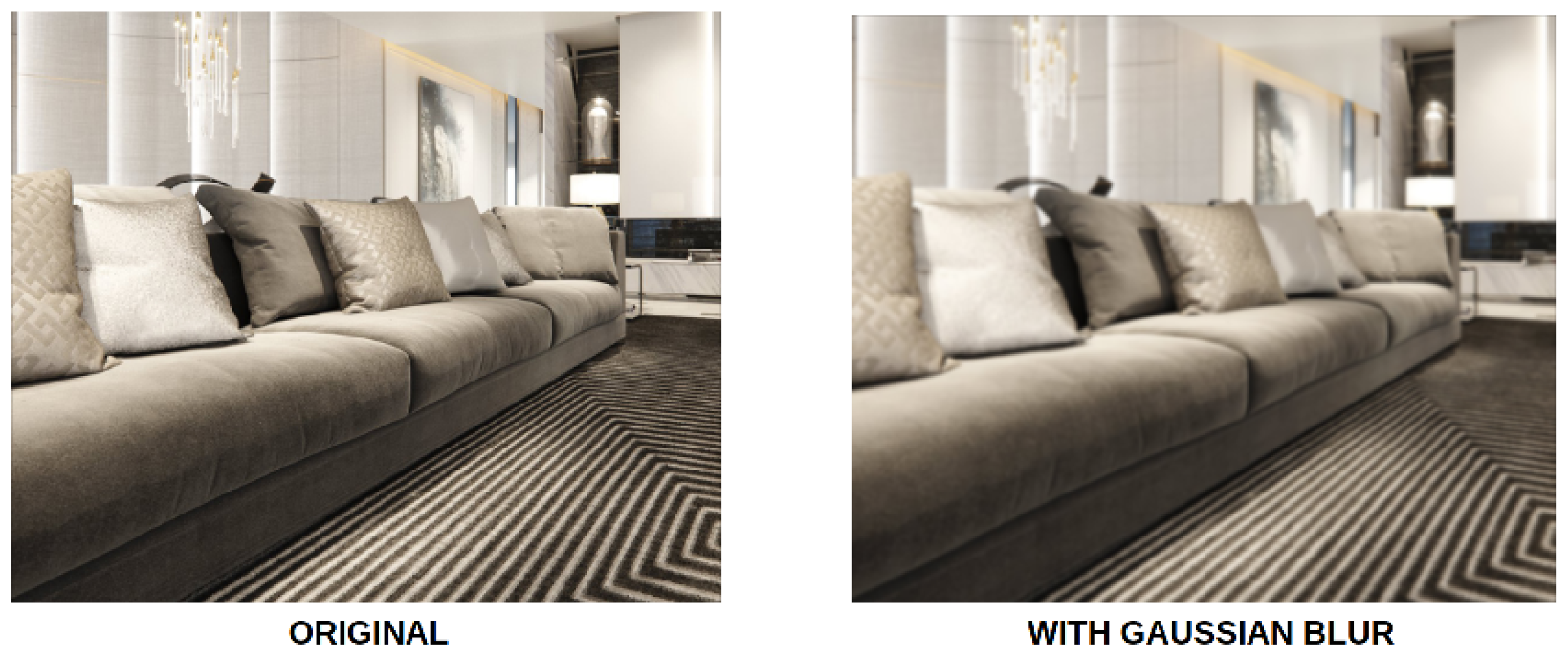
Figure 3.
Example of images before (left, also illustrated in Figure 1, top left) and after (right) applying Gaussian blurring.
Figure 3.
Example of images before (left, also illustrated in Figure 1, top left) and after (right) applying Gaussian blurring.

Figure 4.
An example of the application of the color transfer operation: the color of the source NI in the middle (also shown in Figure 1, bottom right) is transferred to the target CG image on the left (also shown in Figure 1, top right), so as to obtain the color-transferred CG image on the right. The obtained color-transferred image has the visual content of the CG image before the color transfer as well as the color tone of the source NI.

Figure 5.
Modified architecture of ENet to take into account both P local predictions and one global prediction. Here in the illustration, we have .
Figure 5.
Modified architecture of ENet to take into account both P local predictions and one global prediction. Here in the illustration, we have .

Figure 6.
Comparison of the average test accuracy (in %) of classifiers with normal training [5] on the full training dataset and reduced training datasets of different reduction ratios, when trained on Artlantis, Autodesk, Corona and VRay.
Figure 6.
Comparison of the average test accuracy (in %) of classifiers with normal training [5] on the full training dataset and reduced training datasets of different reduction ratios, when trained on Artlantis, Autodesk, Corona and VRay.

Figure 7.
Comparison of the test accuracy (in %) on the four test sets of Artlantis, Autodesk, Corona and VRay, obtained by the baseline normal training [5] and by the combination of the modified new loss and the augmentation of GB (Gaussian blurring) + CT (color transfer). The training was carried out on the Artlantis reduced training set with a 5% reduction ratio.


Table 1.
Experimental results of test accuracy on the four test sets and the average test accuracy (last column, considered as the main performance metric), with networks trained on the full training set of Artlantis. The generalization performances are shown in italic. Here, “aug.” means augmentation. The best result of the average test accuracy is shown in bold.
| Tested on | Artlantis | Autodesk | Corona | VRay | Average | |
|---|---|---|---|---|---|---|
| Methods | ||||||
| Normal training [5] | 98.69% | 89.94% | 85.42% | 88.14% | 90.55% | |
| With aug. NA | 98.75% | 81.25% | 79.31% | 89.44% | 87.19% | |
| With aug. GB | 98.75% | 91.39% | 90.00% | 94.17% | 93.58% | |
| With aug. CJ | 98.89% | 88.06% | 87.92% | 92.36% | 91.81% | |
| With aug. CT | 98.61% | 87.64% | 85.97% | 90.97% | 90.80% | |
| With new loss | 99.58% | 80.56% | 83.61% | 86.11% | 87.47% | |
| With aug. GB + CJ | 98.33% | 89.58% | 91.11% | 95.00% | 93.51% | |
| With aug. GB + CT | 97.64% | 94.31% | 93.75% | 95.14% | 95.21% | |
| With new loss + GB + CT | 99.44% | 89.31% | 89.31% | 93.61% | 92.92% | |
Table 2.
Experimental results of test accuracy on the four test sets and the average test accuracy (last column, considered as the main performance metric), with networks trained on the full training set of Autodesk. The generalization performances are shown in italic. Here, “aug.” means augmentation. The best result of the average test accuracy is shown in bold.
| Tested on | Artlantis | Autodesk | Corona | VRay | Average | |
|---|---|---|---|---|---|---|
| Methods | ||||||
| Normal training [5] | 90.61% | 98.44% | 92.33% | 86.61% | 92.00% | |
| With aug. NA | 89.17% | 98.33% | 88.19% | 87.50% | 90.80% | |
| With aug. GB | 95.56% | 98.33% | 95.28% | 93.89% | 95.77% | |
| With aug. CJ | 90.69% | 98.98% | 95.14% | 92.64% | 94.36% | |
| With aug. CT | 90.28% | 98.75% | 95.28% | 90.42% | 93.68% | |
| With new loss | 91.25% | 98.61% | 95.83% | 90.42% | 94.03% | |
| With aug. GB + CJ | 94.73% | 98.06% | 96.25% | 93.61% | 95.66% | |
| With aug. GB + CT | 94.31% | 97.92% | 96.81% | 94.17% | 95.80% | |
| With new loss + GB + CT | 94.31% | 98.61% | 97.08% | 92.78% | 95.70% | |
Table 3.
Experimental results of test accuracy on the four test sets and the average test accuracy (last column, considered as the main performance metric), with networks trained on the full training set of Corona. The generalization performances are shown in italic. Here, “aug.” means augmentation. The best result of the average test accuracy is shown in bold.
| Tested on | Artlantis | Autodesk | Corona | VRay | Average | |
|---|---|---|---|---|---|---|
| Methods | ||||||
| Normal training [5] | 83.92% | 92.08% | 98.50% | 92.22% | 91.68% | |
| With aug. NA | 87.08% | 91.81% | 97.92% | 95.56% | 93.09% | |
| With aug. GB | 95.28% | 94.58% | 97.50% | 96.67% | 96.01% | |
| With aug. CJ | 88.19% | 92.92% | 98.89% | 95.00% | 93.75% | |
| With aug. CT | 84.44% | 92.64% | 98.89% | 92.08% | 92.01% | |
| With new loss | 89.31% | 94.03% | 99.17% | 93.89% | 94.10% | |
| With aug. GB + CJ | 94.31% | 94.31% | 96.94% | 95.83% | 95.35% | |
| With aug. GB + CT | 96.25% | 95.56% | 97.50% | 95.56% | 96.22% | |
| With new loss + GB + CT | 92.64% | 94.86% | 98.75% | 94.31% | 95.14% | |
Table 4.
Experimental results of test accuracy on the four test sets and the average test accuracy (last column, considered as the main performance metric), with networks trained on the full training set of VRay. The generalization performances are shown in italic. Here, “aug.” means augmentation. The best result of the average test accuracy is shown in bold.
| Tested on | Artlantis | Autodesk | Corona | VRay | Average | |
|---|---|---|---|---|---|---|
| Methods | ||||||
| Normal training [5] | 88.42% | 90.03% | 95.47% | 98.75% | 93.17% | |
| With aug. NA | 90.97% | 84.17% | 93.75% | 97.78% | 91.67% | |
| With aug. GB | 95.97% | 94.72% | 94.17% | 96.53% | 95.35% | |
| With aug. CJ | 89.44% | 87.92% | 96.53% | 97.64% | 92.88% | |
| With aug. CT | 93.19% | 91.39% | 96.81% | 98.33% | 94.93% | |
| With new loss | 94.31% | 92.64% | 95.97% | 98.61% | 95.38% | |
| With aug. GB + CJ | 94.86% | 93.06% | 94.44% | 95.69% | 94.51% | |
| With aug. GB + CT | 97.08% | 95.14% | 96.25% | 97.50% | 96.49% | |
| With new loss + GB + CT | 97.64% | 95.83% | 96.94% | 98.33% | 97.19% | |
Table 5.
The results of the average test accuracy of different methods when trained on the full and reduced training sets of Artlantis. The best result in each column is shown in bold.
Table 5.
The results of the average test accuracy of different methods when trained on the full and reduced training sets of Artlantis. The best result in each column is shown in bold.
| Trained on | Full | Reduced 50% | Reduced 20% | Reduced 10% | Reduced 5% | |
|---|---|---|---|---|---|---|
| Methods | ||||||
| Normal training [5] | 90.55% | 86.84% | 79.61% | 78.30% | 79.41% | |
| With aug. GB | 93.58% | 86.49% | 83.12% | 80.17% | 84.41% | |
| With aug. CJ | 91.81% | 87.47% | 86.60% | 80.77% | 78.20% | |
| With aug. CT | 90.80% | 89.41% | 88.40% | 84.37% | 82.02% | |
| With new loss | 87.47% | 86.11% | 85.10% | 80.52% | 77.99% | |
| With aug. GB + CT | 95.21% | 93.23% | 89.55% | 86.77% | 83.48% | |
| With new loss + GB + CT | 92.92% | 92.61% | 91.32% | 87.12% | 86.81% | |
Table 6.
The results of the average test accuracy of different methods when trained on the full and reduced training sets of Autodesk. The best result in each column is shown in bold.
Table 6.
The results of the average test accuracy of different methods when trained on the full and reduced training sets of Autodesk. The best result in each column is shown in bold.
| Trained on | Full | Reduced 50% | Reduced 20% | Reduced 10% | Reduced 5% | |
|---|---|---|---|---|---|---|
| Methods | ||||||
| Normal training [5] | 92.00% | 90.32% | 84.06% | 79.34% | 73.20% | |
| With aug. GB | 95.77% | 93.58% | 89.83% | 80.73% | 75.35% | |
| With aug. CJ | 94.36% | 91.35% | 87.12% | 82.33% | 76.56% | |
| With aug. CT | 93.68% | 92.92% | 85.00% | 84.38% | 74.79% | |
| With new loss | 94.03% | 92.12% | 87.29% | 81.74% | 77.36% | |
| With aug. GB + CT | 95.80% | 93.27% | 88.68% | 83.47% | 81.39% | |
| With new loss + GB + CT | 95.70% | 96.25% | 87.61% | 87.88% | 82.33% | |
Table 7.
The results of the average test accuracy of different methods when trained on the full and reduced training sets of Corona. The best result in each column is shown in bold.
Table 7.
The results of the average test accuracy of different methods when trained on the full and reduced training sets of Corona. The best result in each column is shown in bold.
| Trained on | Full | Reduced 50% | Reduced 20% | Reduced 10% | Reduced 5% | |
|---|---|---|---|---|---|---|
| Methods | ||||||
| Normal training [5] | 91.68% | 92.33% | 87.57% | 78.79% | 77.12% | |
| With aug. GB | 96.01% | 93.85% | 89.76% | 85.63% | 81.18% | |
| With aug. CJ | 93.75% | 86.60% | 85.84% | 75.52% | 73.78% | |
| With aug. CT | 92.01% | 91.98% | 88.96% | 82.08% | 79.65% | |
| With new loss | 94.10% | 93.09% | 90.38% | 78.72% | 78.02% | |
| With aug. GB + CT | 96.22% | 94.65% | 90.73% | 88.33% | 80.52% | |
| With new loss + GB + CT | 95.14% | 95.00% | 91.18% | 89.00% | 84.72% | |
Table 8.
The results of the average test accuracy of different methods when trained on the full and reduced training sets of VRay. The best result in each column is shown in bold.
Table 8.
The results of the average test accuracy of different methods when trained on the full and reduced training sets of VRay. The best result in each column is shown in bold.
| Trained on | Full | Reduced 50% | Reduced 20% | Reduced 10% | Reduced 5% | |
|---|---|---|---|---|---|---|
| Methods | ||||||
| Normal training [5] | 93.17% | 92.15% | 85.80% | 83.33% | 76.63% | |
| With aug. GB | 95.35% | 92.05% | 87.78% | 86.63% | 82.64% | |
| With aug. CJ | 92.88% | 93.37% | 88.16% | 81.01% | 74.97% | |
| With aug. CT | 94.93% | 92.22% | 89.79% | 84.97% | 80.07% | |
| With new loss | 95.38% | 92.95% | 88.72% | 83.54% | 77.90% | |
| With aug. GB + CT | 96.49% | 96.15% | 93.06% | 89.41% | 82.15% | |
| With new loss + GB + CT | 97.19% | 94.10% | 90.38% | 89.72% | 86.46% | |
Table 9.
Comparison of network training times (in minutes) of different methods when trained on the full Artlantis training set.
Table 9.
Comparison of network training times (in minutes) of different methods when trained on the full Artlantis training set.
| Methods | Training Time | Additional Time Compared to Normal Training |
|---|---|---|
| Normal training | 347 | - |
| With additional enhanced training [5] | 672 | +325 |
| With aug. GB | 356 | +9 |
| With aug. GB + CT | 356 | +9 |
| With new loss | 355 | +8 |
| With new loss and aug. of GB + CT | 368 | +21 |
Table 10.
Comparison in terms of test accuracy (in %) between the state-of-the-art enhanced training method of Quan et al. [5] and our method of the combination of the augmentation of GB + CT, when trained on full training sets. In each pair of results separated by “/”, the former is the result of the method of [5] and the latter is the result of our method. The generalization performances are shown in italic. The best result of the average test accuracy in each row is shown in bold.
| Tested on | Artlantis | Autodesk | Corona | VRay | Average | |
|---|---|---|---|---|---|---|
| Trained on | ||||||
| Artlantis (full) | 97.25/97.64 | 95.69/94.31 | 92.72/93.75 | 94.50/95.14 | 95.04/95.21 | |
| Autodesk (full) | 94.42/94.31 | 97.61/97.92 | 95.14/96.81 | 91.78/94.17 | 94.74/95.80 | |
| Corona (full) | 93.61/96.25 | 92.97/95.56 | 97.86/97.50 | 95.61/95.56 | 95.01/96.22 | |
| VRay (full) | 94.61/97.08 | 93.92/95.14 | 96.83/96.25 | 98.28/97.50 | 95.91/96.49 | |
Table 11.
Comparison in terms of test accuracy (in %) between the method of [10] and our method of the combination of the new loss and the augmentation of GB + CT, when trained on reduced training sets with a reduction ratio of 20%. In each pair of results separated by “/”, the former is the result of the method of [10] and the latter is the result of our method. The generalization performances are shown in italic. The best result of the average test accuracy in each row is shown in bold.
| Tested on | Artlantis | Autodesk | Corona | VRay | Average | |
|---|---|---|---|---|---|---|
| Trained on | ||||||
| Reduced Artlantis (20%) | 96.25/95.00 | 81.39/90.14 | 83.19/87.22 | 84.86/92.92 | 86.42/91.32 | |
| Reduced Autodesk (20%) | 82.36/83.89 | 94.31/96.67 | 82.36/86.39 | 80.56/83.47 | 84.90/87.61 | |
| Reduced Corona (20%) | 80.97/89.17 | 85.00/89.86 | 93.06/93.33 | 87.50/92.36 | 86.63/91.18 | |
| Reduced VRay (20%) | 87.78/89.58 | 82.50/89.86 | 90.00/90.00 | 92.64/92.08 | 88.23/90.38 | |
Disclaimer/Publisher’s Note: The statements, opinions and data contained in all publications are solely those of the individual author(s) and contributor(s) and not of MDPI and/or the editor(s). MDPI and/or the editor(s) disclaim responsibility for any injury to people or property resulting from any ideas, methods, instructions or products referred to in the content. |
© 2024 by the authors. Licensee MDPI, Basel, Switzerland. This article is an open access article distributed under the terms and conditions of the Creative Commons Attribution (CC BY) license (https://creativecommons.org/licenses/by/4.0/).
Share and Cite
MDPI and ACS Style
Bouhamidi, Y.; Wang, K. Simple Methods for Improving the Forensic Classification between Computer-Graphics Images and Natural Images. Forensic Sci. 2024, 4, 164-183. https://doi.org/10.3390/forensicsci4010010
AMA Style
Bouhamidi Y, Wang K. Simple Methods for Improving the Forensic Classification between Computer-Graphics Images and Natural Images. Forensic Sciences. 2024; 4(1):164-183. https://doi.org/10.3390/forensicsci4010010
Chicago/Turabian StyleBouhamidi, Yacine, and Kai Wang. 2024. "Simple Methods for Improving the Forensic Classification between Computer-Graphics Images and Natural Images" Forensic Sciences 4, no. 1: 164-183. https://doi.org/10.3390/forensicsci4010010