
Near-Field Analysis of Turbidity Flows Generated by Polymetallic Nodule Mining Tools


Section of Offshore and Dredging Engineering, Faculty of Mechanical, Maritime and Materials Engineering, Delft University of Technology, 2628 CD Delft, The Netherlands
*
Author to whom correspondence should be addressed.
Mining 2021, 1(3), 251-278; https://doi.org/10.3390/mining1030017
Submission received: 28 September 2021
/
Revised: 20 October 2021
/
Accepted: 25 October 2021
/
Published: 1 November 2021
(This article belongs to the Topic Deep-Sea Mining)
Abstract
:The interest in polymetallic nodule mining has considerably increased in the last few decades. This has been largely driven by population growth and the need to move towards a green future, which requires strategic raw materials. Deep-Sea Mining (DSM) is a potential source of such key materials. While harvesting the ore from the deep sea by a Polymetallic Nodule Mining Tool (PNMT), some bed sediment is unavoidably collected. Within the PNMT, the ore is separated from the sediment, and the remaining sediment–water mixture is discharged behind the PNMT, forming an environmental concern. This paper begins with surveying the state-of-the-art knowledge of the evolution of the discharge from a PNMT, in which the discharge characteristics and generation of turbidity currents are discussed. Moreover, the existing water entrainment theories and coefficients are analyzed. It is shown how plumes and jets can be classified using the flux balance approach. Following that, the models of Lee et al. (2013) and Parker et al. (1986) are combined and utilized to study the evolution of both the generated sediment plume and the subsequent turbidity current. The results showed that a smaller sediment flux at the impingement point, where the plume is transformed into a turbidity current, results in a shorter run-out distance of the turbidity current, consequently being more favorable from an environmental point of view.
1. Introduction
The industrial revolution and the rising living standards around the world require an unconventional search for resources for many key materials (e.g., Cobalt (Co), Nickel (Ni), Tellurium (Te), Titanium (Ti), Platinum (Pt), and rare Earth metals). These raw materials are vital to many modern industries (e.g., wind turbines, telecommunications, and computers) [1,2]. However, the continuous decrease of the grade of these minerals on land makes it worthwhile for mining companies to go into the deep ocean, which has the advantage of having better ore grades [3], for instance researchers estimated that the largest reserves of cobalt, nickel, and manganese are found on the sea bed [4]. However, Deep-Sea Mining (DSM) requires the consideration of several technical aspects, and these should be compatible with the targeted mineral deposits, seabed conditions, water depth, collection method, and deep-sea fauna [5] (see Figure 1).
The DSM system for polymetallic nodules consists of three parts, namely the Hydraulic Polymetallic Nodule Mining Tool (PNMT), the Vertical Transport System (VTS), and the Production Support Vessel (PSV). Deep-ocean polymetallic nodules form on or just below the abyssal plains of the ocean. An enormous amount of nodules is located on the ocean bed at a depth of approximately 4300–5500 [2]. Regarding polymetallic nodule mining operation, the PNMT collects the nodules from the sea floor and primarily separates the nodules from the excess water and fine sediments, which are discharged directly at the seafloor. Next, the VTS transports the collected nodules from the sea bed to the PSV at the sea surface, where the collected ore is dewatered. Finally, the VTS is used again to return the transported water, containing Sediments, Waste, and Other Effluents (SWOEs) to the deep sea. Figure 1 shows a typical scenario for a DSM system. There are two main sources of sediment plumes generated by DSM activities:
- (i)
- The discharge of the sediment–water mixture from a PNMT, which remains after the separation process [6];
- (ii)
The released suspended sediment, whether it is from the VTS or from the PNMT, forms a sediment cloud termed a “sediment plume”. This plume increases the turbidity level of deep-sea water [9,10], which negatively impacts the marine ecosystem [11]. In other words, fish behavior is affected, and the mortality rate of zooplankton species increases [11]. Additionally, the fresh deposited sediments from the discharged plume on the sea bed clog the feeding paths to sea bed benthic organisms. Evidently, DSM requires an accurate evaluation of its environmental consequences [2,12].
The effect of sediment disturbance resulting from DSM applications on the local physicochemical conditions, i.e., soil composition and organic carbon content, of the disturbed area was investigated experimentally by [13]. The physical parameters (e.g., velocity and concentration profiles) of sediment plumes resulting from dredging operations were studied by [14,15]. The work of [7] documented numerical and experimental results of plume discharge from a VTS. A CFD analysis was performed by [6] for a horizontal discharge from a PNMT to investigate the effect of different discharge conditions (see the controlling parameters of a discharge process in Section 2.2) on the plume dispersion. A preprototype PNMT was developed and tested in the Belgian and German exploration areas; based on the results, a comprehensive monitoring program for the local environment was developed [16]. The work of [17,18] showed that the Particle Size Distribution (PSD) governs the traveling distance of fine suspended sediment. They found that the particle size changes as a result of the aggregation–breakup process between sediments (see Section 6 for more details about the flocculation process).
In the last few decades, valuable insight has been gained into DSM processes through various projects, where the environmental impacts of DSM were investigated, e.g., Refs. [5,9,10,13,17,19,20,21,22,23]. Some of the DSM research projects are mentioned as follows:
- The Deep Ocean Mining Environmental Study (DOMES) project was one of the leading projects, which aimed to obtain and investigate the necessary data for an independent impact assessment of DSM activities. DOMES was divided into two main phases as follows [19]:
- (i)
- Gaining quantitative data on the biological communities prior to mining and developing a framework to predict the impact of manganese nodule mining on the marine environment;
- (ii)
- Determining the accuracy of the environmental impact predictions obtained in the first phase through monitoring of pilot mining tests.
As a result of this project, a quantitative baseline of environmental parameters and a predictive framework were developed to characterize DSM environmental impacts. Furthermore, preliminary environmental guidelines for DSM were defined; - The Marine E-tech project took place in the Tropic Seamount in the north east Atlantic near the Canary Islands and aimed to study the environment sensitivity to Fe-Mn crust DSM operations. The Fe-Mn crusts are differentiated from polymetallic nodules as a result of different locations, depths, and DSM operation techniques. The local influencing variables (e.g., temperature, pressure) that govern the composition and formation of the Fe-Mn nodules were investigated. A Remotely Operated underwater Vehicle (ROV) was used to generate sediment plumes, and the plume dispersion was studied. The measurements showed that the plumes were significantly smaller than predicted because the effect of flocculation was not taken into account [17];
- The Towards Responsible Extraction Of Submarine Mineral Resources (TREASURE) project studied SWOE discharge from a VTS [22]. Within the scope of TREASURE, numerical simulations were performed using the drift-flux modeling approach (for details on drift-flux modeling, see [24]) to predict the VTS discharged plume characteristics (e.g., velocity and concentration) [25]. In addition, Reference [7] carried out detailed laboratory experiments to test different discharge parameters such as initial concentrations, momentum, and distance from the bed on the plume dispersion. The numerical results (e.g., velocity and concentration profiles) were compared against the experimental results, and a good agreement was found between them;
- The PLUMEX2018 field experiments were conducted in the Southern California Bight at the beginning of 2018 [26]. The Multiresolution primitive equation regional ocean modeling system (MIT-MSEAS) model was used to predict the plume dispersion, i.e., direction, velocity, and concentration. Good agreement was found between the MIT-MSEAS model and the PLUMEX field experiments [23];
- The JPI-Oceans Mining Impact II research project aimed to develop a new framework for environmental monitoring and predictions for the environmental impacts of mining operations [27]. Global Sea Mineral Resources (GSR), a subsidiary of DEME group, designed and tested a PNMT in the Clarion-Clipperton Fracture Zone (CCFZ) within the Belgian license area to assess its environmental impact [16]. GSR performed detailed measurements on the current environment (climate, geomorphological, physical oceanographic, seabed substrate characteristics, natural hazards, noise, and light). Moreover, a biological baseline was assessed based on habitat heterogeneity. The potential environmental impact was divided into six categories:
- (i)
- Habitat/nodule removal;
- (ii)
- Plume formation;
- (iii)
- Biogeochemical changes of the sediment particles;
- (iv)
- Potential release of toxic sediment into the lower water column;
- (v)
- Emissions to the air;
- (vi)
- Natural hazards (weather condition, storms).
The objective of this paper is to present an analysis of the characterizations of plumes generated by a PNMT in terms of the transport, spreading, and deposition of sediments. This will help determine the optimal discharge conditions to minimize the environmental impact caused by sediment plumes. In this regard, the emphasis will be on the near-field effects (see Section 2.1 for the near-field/far-field definitions), where engineering and the design of equipment can significantly influence the spread and deposition of the generated plume.
This paper proceeds as follows. Section 2 provides an overview of the discharge process and the key parameters controlling it. In Section 3, we present the relevant length and time scales associated with polymetallic nodule mining process and an overview of sediment-laden jets and plumes. Section 4 presents the most important physical aspects of the jets, plumes, and turbidity currents analyzed herein. In Section 5, the model of [28] and the four-equation model of [29] are employed to study the mining-generated plume and subsequent turbidity currents. Section 6 discusses the flocculation effect on the discharged turbidity current. Finally, Section 7 provides key directions for future research.
2. Discharge Process
In this section, we first present an overview of the PNMT discharge process in order to study the turbidity flows generated by DSM. Secondly, a classification of the discharge properties and the physical parameters of the PNMT discharge process are described.
2.1. Overview
The main differences between the two discharge sources in a polymetallic nodule mining operation are the orientation (vertical from the VTS and mostly horizontal from the PNMT), distance to the seabed, flow rate, and concentration of the suspended sediments. Some studies showed that the SWOE discharge location ranges from near the seabed to just below the oxygen minimum layer (800–1000 m water depth) [5,7,8,21], while the distance to the seabed of a PNMT depends on the discharge position on the PNMT, ranging from 1–3 m. The SWOE discharge flow rate and concentration are estimated to be about 0.56 m/s and 8 g/L, respectively [21,23]. Table 1 shows the estimated solid flux rate and sediment concentration range of a PNMT discharge.
Bed disturbances mainly result from the movement of a PNMT and the pick-up process [13], which could be hydraulic, mechanical, or hybrid. A benthic disturbance experiment mimicking PNMT disturbances was conducted to investigate particles’ resettlement on marine ecosystems during DSM operation [13]. They found that the particles migrate to the adjacent areas outside the mining zone, causing a change in the physicochemical bed properties. These migrated particles potentially clog the feeding paths of the benthic organisms.
Discharging these sediment–water mixtures without carefully optimizing the discharge parameters might unnecessarily enlarge the area affected by plume dispersion. A few studies are found in the current body of research about the discharge process from the PNMT, e.g., [6]. In this respect, we present in Section 5 our investigation of the sediment–water discharge from a PNMT. We divided the horizontal discharge of a sediment–water mixture from a PNMT into four main parts of interest as follows (see Figure 2):
- 1.
- Discharge source: This contains the initial conditions such as the momentum, concentration of suspended sediments, and distance from the sea bed z. The physical parameters depend on the design of the PNMT (e.g., methods of collection and separation);
- 2.
- Jet or plume regime: In this region, depending on the flow discharge parameters, the flow can be a jet or plume. Later, when the buoyancy force is dominant, the flow becomes a plume (see Section 2.2 and Section 4.2);
- 3.
- Impingement region: This region is located on the sea bed. Here, the negative buoyant plume changes its direction due to the direct interaction with the seabed. Sediment deposition and possible sea bed erosion are expected to take place within this region;
- 4.
- Turbidity current: This current is formed beyond the impingement region.
In the literature, classifying of sediment plumes is often related to length and time scales. Accordingly, terms such as near-field or far-field regions are defined as follows (see Figure 3 and Figure 4):
- Near-field region: This defined as the region close to the discharge apparatus, and it is mostly controlled by the discharge conditions. The flows in this region have a typical length scale up to few hundreds of meters and a time scale in the range of seconds to minutes;
- Far-field region: This is defined as the region where the plume trajectory is dominated by the environmental parameters, such as the currents and seabed topology. The flows in this region have large time and length scales, which are typically in the range of days and kilometers, respectively.
2.2. Physical Parameters
- (i)
- Mixture properties;
- (ii)
- Ambient conditions;
- (iii)
- Geometrical conditions.
Concerning the mixture properties, the sediment–water discharge parameters (momentum, buoyancy, and volume) control the flow regime at the discharge source. The sediment plume dispersion is highly dependent on the ambient conditions, such as the turbulence level and background stratification, which are of high importance to quantify the plume dispersion within the near-field/far-field regions. The discharge geometry and its orientation are two of the key aspects that need to be well considered during the design process of a PNMT.
The discharge source is defined as the release point of the sediment–water mixture at the back of a PNMT. The source condition is characterized by the momentum flux , buoyancy flux , volume flux , and reduced gravity of a mixture. These parameters are determined as follows:
where A is the cross-sectional area of the discharge geometry; , where is the ambient density, is the discharge density, and is the discharge velocity. The Boussinesq approach neglects the density difference, while the non-Boussinesq approach assumes a difference in density between the discharged and ambient flows. The turbulence level is indicated by the Reynolds number (). Furthermore, the ratio between the inertial force and the gravitational force represents the densimetric Froude number (), which classifies the discharged flow into different flow regimes (, critical flow, , supercritical flow, , subcritical flow). The mixing process of a buoyant jet can be classified based on the Richardson number (); if , the flow is dominated by buoyancy, whereas if , the flow is dominated by momentum [35].
where is the dynamic viscosity and L is the characteristic length, which is calculated based on the discharge geometry in the discharge origin (see Figure 2). A design framework characterizing the discharge process of the sediment–water mixture generated by PNMT is needed to analyze the sediment plume dispersion and the characteristics of the formed deposition layer. Besides the discharge defining, the nodule pick-up and separation processes have a great importance in controlling the initial conditions of the sediment–water discharge parameters (see Equations (1)–(5)). These processes highly affect the mixture discharge, i.e., increased erosion of the sea bed leads to a high flux of sediments at the discharge source.
3. Flow Specification
Different flow regimes (e.g., jet, plume, and turbidity current) are expected in the near-field area, and these depend on the discharge parameters described in the previous section. These flow regimes occur within certain length and time scales. We here present the expected length and time scales for the underlying physical processes associated with a polymetallic nodule mining process. Moreover, we provide an overview of the physics governing sediment particle suspensions and a brief review of sediment-laden jets and plumes.
3.1. Length and Time Scales
The characteristic length and time scales in DSM applications vary over a wide range of magnitudes. Figure 3 and Figure 4 represent the expected length and time scales associated with a polymetallic nodule mining process. For a dimensional analysis, the most important length scales of a discharge process are the momentum length scale and the buoyancy length scale [34,36], where is defined as the distance where the momentum of the discharge is dominant, i.e., jet-like, and is defined as the distance where buoyancy is dominant, i.e., plume-like [37]. In other words, represents the distance at which the flow velocity decreases to the ambient velocity [34]. Regarding jet flow, there is an established jet core near the discharge source, which is not affected by the ambient entrainment. Therefore, Reference [36] divided the jet region into two zones: Zone of Flow Establishment (ZFE) and Zone of Established Flow (ZEF) (see Figure 6). A Lagrangian model was presented by [36] for a buoyant jet, which can predict the ZEF and ZFE. Far from the discharge source, buoyancy forces dominate the flow. Mining operations affect the mined areas; however, the turbidity current resulting from the discharge process might also affect the region beside the mined area, as it could potentially travel for a long distance. Recently, using an industrial-scale particle transport model, Reference [18] estimated this distance to be in the range of 4–9 km.
3.2. Particle-Laden Plumes
3.2.1. Particle Physics
Different ranges of particle size are encountered in DSM projects. This section outlines the main physics of a moving particle in a flow and the hindered settling concept.
A single spherical particle settling in a quiescent and an infinite domain is governed by five forces: the drag , gravitational , buoyancy , added mass , and history forces [24,38] (see Figure 7).
The added mass force and history force can be omitted in the scope of this work, because these forces are considered unsteady terms and less significant compared to the other forces. Hence, the particle motion equation can be expressed as follows [24]:
where and are the projected area of the particle and the particle size, respectively, is the drag coefficient, is the velocity of the particle, u is the carrier fluid velocity in the vertical direction, is the carrier fluid density, is the particle mass, and g is the gravitational acceleration. The drag coefficient has many formulas in the literature depending on the particle shape and roughness. These formulas were collected and classified according to the particle Reynolds number [39]. The particle Reynolds number is the ratio between the particle inertial and viscous forces; moreover, it is a key parameter in determining particle motion. It is worth mentioning that these formulas were derived for spherical particles. The shape of the particle has a strong influence on the motion of the particle. A general expression for the settling velocity was derived by [40] as follows:
where is the kinematic viscosity, , is the particle density, is the carrier fluid density, is reported according to particle shape and lies between the value of , and is the drag coefficient, for spherical particles and for nonspherical particles.
The Stokes number () represents the ratio between the particle response time (the time taken by a particle to adapt to the fluid motion) and the hydrodynamic time scale (, where L is the typical length scale and u is the flow velocity at this length scale).
In the case of small particles, , the particle is guided by the flow motion, whilst for big particles, , the flow does not affect the particle motion [24].
Hindered settling represents the reduction of the settling velocity due to the interaction of the particle with the neighboring particles (i.e., collisions, displaced water, group settling). Based on sedimentation and fluidization experiments, Reference [41] calculated the hindered settling velocity for individual particle suspended within a mixture as follows:
where is the hindered settling function depending on and is the hindered settling velocity, which is related to the volumetric mixture concentration . According to [41], the hindered settling function considers the particle Reynolds number and the concentration value as follows:
where n is called the Richardson and Zaki index, and it depends on the Reynolds number of the particles.
Polymetallic nodules are abundantly available in the Clarion-Clipperton Fracture Zone (CCFZ) region, which is located in the Pacific Ocean [21]. Sediment in the CCFZ consists of several fractions such as biogenic ooze, terrigenous or pelagic clay, volcano debris, hydrogenous material, and metalliferous sediment.
The Blue Nodules project is a Horizon 2020 project (EU Research and Innovation Program), which ran between February 2016 and July 2020. The project aimed to develop and test a novel PNMT in the CCFZ region. Within the scope of the Blue Nodules project, NTNU (Norwegian University of Science and Technology), a partner in the project, analyzed the obtained CCFZ sediment samples. The sediment compositions for different sites in the CCFZ are compared in Table 2 and Table 3, where BC064 and BC062 are two box core samples obtained from the GSR contract area. Interoceanmetal Joint Organization (IOM) data were collected from IOM license area, which is located in the eastern part of the CCFZ [42,43]. For further details on CCFZ sediment composition, the reader is referred to the Blue Nodules project public reports and GSR public reports [16,42,43,44].
3.2.2. Sediment-Laden Jets and Plumes
A fundamental understanding of the physical parameters of discharge, e.g., velocity, concentration, and turbulence, is needed to investigate the effect of the PNMT discharge on the sea environment. An increasing particle deposition rate and reducing plume dispersion rate would minimize the environmental impact.
Bleninger et al. (2002) [46] and Neves et al. (2002) [47] carried out small-scale experiments on horizontal jet discharges to measure the particles’ deposition. A large scatter in the deposition rate measurements was noted due to difficulties in ensuring a constant concentration discharge and steady-state flow rate during the discharge process. Lab experiments were conducted to study the sedimentation from horizontal and inclined buoyant jets in a stationary environment [48]. They introduced an integral model to determine the deposition behavior from an inclined, turbulent, buoyant jet. A dimensionless fall speed parameter, i.e., defined as the ratio between the settling velocity and the entrainment velocity, was incorporated into the model to measure the dependency of the source velocity on the deposition near the discharge source. The model was validated with laboratory experiments where the deposition behavior, plume shape, and sedimentation near the source were assessed. The earlier experiments on sediment-laden jets and plumes had the potential pitfall of not sustaining the steadiness of concentration and uniform shape at the jet exit [28].
A theoretical Lagrangian model of horizontal jets discharged in a stationary environment was presented by [28]. They investigated the deposition mechanisms of a horizontal particle-laden jet in terms of longitudinal distance and spreading angle. Their Lagrangian model was used by [49] to validate the experimental work of [28,48,50]. This model is adopted in this work in Section 5.
The impingement region (Figure 2) entails a complex behavior of the flow due to the interaction between the discharged mixture and the ocean bed. At this region, the flow makes a turn and converts from a plume to a wall-bounded flow (i.e., turbidity current [51]), due to the presence of the ocean bed. This current propagates downstream of the ambient flow and interacts with the bed.
3.3. Turbidity Current
Turbidity currents can be described as particle-laden underflows, which are driven by the excess hydrostatic pressure resulting from the density difference between the ambient water and the sediment–water mixture [52,53]. Within this current, turbulence is developed due to the continuous motion of the current over the bed and the generated shear stresses as a result of the mixing process with the ambient water at the upper boundary of the current.
Turbidity currents can be triggered by several phenomena, such as internal waves or tides [54], river plumes [55], and breaching flows slides [56]. The mining process by a PNMT is also expected to trigger a turbidity current at the impingement region by the sediment–water discharge. Here, we refer to this current as a mining-generated turbidity current. The interaction between the discharge and the seabed determines the behavior of the generated turbidity current; the hydraulic properties prior to the impingement region are the main information to characterize the generated turbidity current.
Turbidity currents can occur in turbulent and laminar regimes. The flow regime is classified with the Reynolds number (flow thickness is the characteristic length scale), where is laminar; above that, the flow is turbulent. The deposition and resuspension of sediment is highly affected by the turbulence structure [53]. Turbidity currents are divided into three parts: head, body, and tail (see Figure 8). From the perspective of hydraulics, the head has different properties than the region behind it (body and tail) [57,58]. The mass and momentum at the head differ significantly from the body and tail, as the head displaces the ambient fluid. Hence, the head is the densest part, as it experiences a friction resistance. Furthermore, the head is considered a “locus of erosion” [57,59], impacting the deposition and bed morphology. The head forms a nose starting at the lower region due to the no-slip boundary condition at the bed and the friction resistance at the upper region [60]. At the back of the head, vortices start to take place due to the effect of the velocity shear and turbulence in the ambient fluid. These vortices define the dynamics of the head and can be identified as Kelvin–Helmholtz instabilities [61]. As a result of these instabilities, the back of the head forms a sharp discontinuity in the thickness of the current. However, the average velocity of the body region has to be larger than the forward velocity of the head to achieve a constant rate of advance. [57]. The entrainment of the ambient fluid into the turbidity current and the change in the amount of suspended solids, due to net erosion or net deposition at the bed, depend on the characteristics of the current, and these also lead to changes in velocity, concentration, and particle size over time. Based on the velocity and concentration profiles, it is possible to derive characterizing layer-averaged parameters of a turbidity current. Parker et al. (1987) [62] derived a set of equations to estimate the layer-averaged characteristics for a turbidity current as follows:
where is the layer-averaged velocity, h the height of the current, the layer-averaged concentration, the upward normal coordinate, the local concentration, the local velocity, and z the vertical coordinate.
Many mathematical models are available to describe the phenomenon of turbidity current. These models can be divided into two main categories [57]. The first category is based on the vertical averaging technique, which describes the velocity and concentration with a single point (layer-averaged magnitude) along the traveling distance of the current. The characterization of the structure of each model depends on the assumptions made for the conservation of these flow parameters. The conservation of momentum as one equation model was used in the work of [63], while [64] involved four equations, i.e., conservation of mass, momentum, sediment mass, and energy equations, to derive his model.
The second category drives the whole velocity and concentration profiles from a turbulence model. The equations of the total kinetic energy k and its dissipation have been used as a turbulence closure. Spatial averaging (large eddy simulation) can also be used as a closure for the turbulence [65,66,67,68].
4. Flow Physics
The literature reports many physical approaches that characterize the flow physics in the near-field region. Here, we describe the most important physics governing the discharged flow in the near-field region. We also summarize the differences between the Gaussian and top-hat approaches, which were used in previous studies of plume integral models. Moreover, we outline the flux balance approach, the entrainment theory, and the turbidity current.
4.1. Gaussian and Top-Hat Profiles
Many researchers [69,70,71,72,73,74] used integral models to describe the physics of plumes. Gaussian and top-hat profiles are the main assumptions for these models. The study of [75] extensively compared the governing equations of plumes using Gaussian and top-hat assumptions. The top-hat profile uses a constant velocity and concentration distribution over the entire plume domain, where the velocity and concentration are the average values of the dominant eddies (see Figure 9). Additionally, the large eddies within the plume are responsible for the overall transport of momentum and mass, while the small eddies have no effect. Top-hat profiles are used mostly in the Lagrangian approaches [36]. On the other hand, the Gaussian profile uses a Gaussian function to describe the velocity and concentration profiles, which are more suitable for Eulerian approaches [36]. Using the top-hat assumption would lead to a larger entrainment coefficient compared to the Gaussian profile [76].
Describing the plumes’ spreading behavior using the top-hat profiles offers an analytical simplicity because of the simple equations that can be used directly at the source and do not need any prior treatment for the initial condition (momentum, buoyancy, volume fluxes). Gaussian and top-hat approaches are crude assumptions to describe the self-similarity of the plumes [75]. Furthermore, the difference between these two approaches is small in terms of the predictions of the physical parameters. Moreover, the additional physical parameters that come within the Gaussian analysis have a minor role in describing the mean plume characteristics.
Various cases of turbulent jet geometries, e.g., slot and round shape, were studied in the work of [28]. They illustrated the governing equations that describe the jet propagation, i.e., velocity and concentration profiles along the jet width, for each of these cases. They provided an analysis for a turbulent jet from a slot in which the velocity and the concentration profiles are described by a Gaussian function (2D, x-y, Cartesian coordinates).
4.2. Flux Balance Approach
Flux balance parameter is an analytical parameter that introduces a theoretical framework of plumes [78]. The flux balance parameter is defined as the ratio of buoyancy force to inertia force [69]. The flux balance parameter can be expressed as follows [78]:
where , , , and are the initial flux balance, buoyancy, mass, and volume fluxes, respectively, is the entrainment coefficient (see the entrainment theory in Section 4.3), and is the initial momentum flux under the Boussinesq approximation.
Using the flux balance parameter, based on the discharge conditions, it is possible to classify the discharged flow into different regimes as follows:
- (i)
- is a pure plume.
- (ii)
- is a forced plume.
- (iii)
- is a lazy plume.
- (iv)
- is a pure jet.
The plume is considered pure when its momentum and buoyancy fluxes are the same at the discharge source [79]. The plume is regarded as lazy when its buoyancy forces are dominant at the discharge source [80], while the plume is regarded as a forced plume (also known as a buoyant jet) when its momentum forces are dominant at the discharge source [70]. The pure jet remains a jet until it dissipates due to viscous diffusion [79].
Additionally, can be introduced as a square ratio between the source length and jet length , i.e., the momentum-dominated region [81].
where, for Boussinesq plumes:
and for non-Boussinesq plumes:
4.3. Water Entrainment Theory
Jets and plumes are shear flows generated by buoyant and inertial sources. The interaction of jets and plumes with the surroundings is known as the entrainment process. The development of a jet or a plume causes a velocity shearing that creates turbulent eddies that entrain the surrounding fluid [79]. The integral models of turbulent jets and plumes use the entrainment hypothesis as a closure relation for the turbulence. The entrainment hypothesis links the entrainment velocity , the rate at which ambient water is entrained across the edge of turbulent plume, to the characteristic velocity of the plume by a single coefficient of proportionality, , which is called the entrainment coefficient [69,82,83]. The entrainment velocity is calculated as follows:
where is the ratio of the plume density to the ambient density. The classical approach of the entrainment hypothesis is based on the macroscopic conservation of momentum, mass, and volume fluxes. It has also a self-similar behavior of the turbulence in a dimensionless form over the downstream distance from the source [69]. A range of entrainment coefficients values (see Table 4) for different authors have been reported in the literature [84]. The entrainment coefficient ranges are 0.10 0.16 for plumes and 0.065 0.080 for jets (these values were calculated assuming a top-hat profile and a self-similar behavior of the plume) [84]. The variations in occur due to the different setups of the experiments and the resulting experimental error. The systematic differences between the reported values of for plumes and jets suggest that depends on the ratio between buoyancy and inertia ( parameter; see Section 4.2).
As mentioned above, the entrainment coefficient is the only parameter that represents the turbulence effect on the mean flow parameters. In this regard, Reference [85] proposed imposing restrictions on the entrainment coefficient by the mean kinetic energy equation. These restrictions are referred to as the entrainment relation. This relation couples the entrainment coefficient to the physical process, such as the buoyancy effect and turbulence production, while the entrainment models are closure relations, which are obtained after all the coefficients of the entrainment relation are parameterized [69,86].
The mathematical models of [69,86] were developed by the integration of time-averaged Navier–Stokes equations across a plane perpendicular to the mean flow direction (axial cross-section). The result of this integration is a system of coupled ordinary differential equations. The mathematical model of [69] depends on the volume flux, momentum flux, and buoyancy flux, while [86] based their model on the momentum, buoyancy, and mean kinetic energy, where the equations of [86] rely on the turbulence kinetic energy and Reynolds stresses. A few years later, Reference [87] presented a theory on an isolated plume in still air, and a new hypothesis was formulated in which the turbulence intensity directly affects the entrainment coefficient. Hence, a new equation was added to solve the turbulence kinetic energy. Utilizing the works of [69,86], the momentum, buoyancy, volume, and kinetic energy conservation equations were combined [88]. This was the first attempt to impose the constraints on based on the conservation of kinetic energy.
Plumes and jets are conical shapes that develop in a self-similar fashion [78]. Rescaling dependent variables on the radial coordinate using characteristic scales such as velocity , buoyancy , and local width is a way to view the self-similarity [89]. The effective entrainment radius and effective density parameter for Boussinesq and non-Boussinesq flows were introduced as follows [90]:
A self-similar solution for the plume characteristics from the governing equations in the z coordinate of steady-state plumes with the top-hat profile was derived as follows [90]:
A method to calculate the characteristic scales, which does not rely directly on the Gaussian shape assumption, but on the flow integral quantities, was proposed as follows [89]:
M and Q are the momentum and volume fluxes, respectively, and B is buoyancy in the integral form [91].
Integrating the continuity equation from the work of [69] over the radial direction leads to the dilution in jets and plumes:
Here, is the entrainment volume flux into a plume or a jet per unit height and is a dimensionless vertical coordinate equal to . From the entrainment assumption (), the next equation can be derived:
5. Assessment of the Near-Field Generated Plume and Turbidity Currents
In this section, we investigate the effect of all properties of the sediment–water mixture discharged from a PNMT on the hydrodynamics of the generated plume and turbidity current. This eventually aims at selecting the optimal discharge scenarios from an environmental point of view.
In our modeling approach, we considered that we have two separate, but connected regions. The first region entails the trajectory of the plume starting from the discharge source and ending at the impingement point, while the second region includes the generation and evolution of a turbidity current downstream the impingement point (see Figure 2). The governing equations of these two regions and the numerical results are presented in the following subsections.
5.1. Lagrangian Plume Model
The two-layer Lagrangian jet model, which was developed by [28], was used here to simulate the evolution of the jet/plume from the discharge source until the impingement point at the seabed. This model was validated by [49] against the experimental results of [28,48,50], justifying our choice of this model. The Lagrangian formulation approaches a changing cross-section and a coordinate system that both march in time with discrete time steps. The model follows a slicewise approach, meaning that there is a plume slice at each time step (see Figure 10), which has its unique characteristics, assuming a uniform top-hat profile.
The discharge trajectory depends on water entrainment, plume bending, and plume growth. The entrainment flux was calculated using Equation (34), and the entrainment coefficient was calculated based on the densimetric Froude number using Equation (33) [92]. The initial angle of the plume at the discharge source is (with the horizontal axis), and the initial mass of the plume can be calculated using , where a is the slice width and is the slice length. The time step was calculated based on the initial velocity magnitude and initial diameter, and it was consistent throughout the marching procedure. The subscripts 0, i, and denote the quantities of the initial condition, previous time step, and current time step, respectively. Following [49], the governing equations are expressed and solved in the following sequence:
where u and w are the velocities in the x and z coordinates, respectively, and is the volumetric concentration.
5.2. Four-Equation Model for Turbidity Currents
The layer-averaged, four-equation model of [29] was developed by integrating the four conservation equations of momentum, fluid mass, sediment mass, and turbulent kinetic energy over the height of the turbidity current. The water entrainment, shear stress, and sediment entrainment were included as source terms. Following [93], the four equations can be expressed as follows:
where h is the current height, is the bed slope angle, Ri is the Richardson number, U is the layer-averaged velocity, C is the layer-averaged concentration, K is the layer-averaged turbulent kinetic energy, is the layer-averaged mean rate of turbulent energy dissipation, n is the bed porosity, is the water entrainment coefficient for turbidity currents, is the net erosion velocity perpendicular to the bed surface resulting from the combined effects of deposition and erosion, and is the hindered settling velocity. The bed shear velocity is calculated by the relation in which is a constant (0.05 to 0.5). The water entrainment coefficient is calculated as follows [29]:
and is calculated using the relation:
where is a dimensionless parameter and is a pseudo friction coefficient.
The erosion velocity for clay is calculated using the relation presented in [94] as follows.
where is the consolidation/swelling coefficient, is a factor equal to 10, is the undrained shear rate, is the bed shear stress, and is the critical shear stress in which is the plasticity index and = 0.7 Pa for 0.35 1.4 Pa.
To account for sediment deposition, the sedimentation velocity is calculated , in which is the near-bed volumetric sediment concentration and is estimated by the relation in which is a dimensionless parameter. The settling velocity for a single particle is calculated based on Equation (10), and hindered velocity is calculated based Equation (12) as follows:
Note that more advanced models can be used for the numerical computations of turbidity currents. Nonetheless, we used a simple model in our analysis, as our objective was to study the relationship between the initial conditions at the discharge source and the run-out distance of the mining-generated turbidity current, rather than obtaining precise results.
5.3. Model Application
Figure 10 shows the case considered in the numerical simulations. The origin of the z coordinate was at the center of the discharge source. The streamwise coordinate in the downstream region is denoted as s.
A typical forward velocity of a PNMT ranges between 0.25 m/s and 0.5 m/s. To reduce the environmental effect of the discharge, engineers aim to have a discharge velocity equal to the forward velocity of the PNMT. In our analysis, therefore, we considered a stationary PNMT with two discharge velocities of 0.25 m/s and 0.5 m/s and three different scenarios for the volumetric discharge concentration: 1.5%, 2%, and 2.5%. The corresponding diameters of the discharge, which result in identical volumetric suspended sediment transport rates per unit width , were 0.45 m, 0.34 m, and 0.27 m, respectively.
At the impingement point, the flow makes a sharp turn, and a turbidity current is formed, which travels downstream and interacts with the bed surface. Consequently, depending on the conditions, net erosion or deposition upon the bed could take place. For simplification, we assumed that we have a complete transfer of the plume characteristics to the downstream region, which has a constant bed slope angle of 3, in agreement with the average slope found in the eastern part of the Clarion-Clipperton Zone (CCZ) [16].
Table 5 summarizes the sediment properties used in the numerical computations. Most of these properties were obtained from the technical report of Global Sea Mineral Resources NV on the field experiments conducted in the eastern part of the CCZ [16]. Note that the non-Newtonian aspect was not considered in our numerical analysis, but it might be relevant for real cases.
5.4. Comparison of the Results
For simplicity, we assumed that the run-out distance of the turbidity current was the main criterion to assess its environmental harmfulness. Additionally, a turbidity current of a lower volumetric suspended sediment at the end of the considered numerical domain tends to die out earlier and thus has a shorter run-out distance. As this paper deals with the near-field flows, we analyzed the results up to 100 m downstream the impingement point.
Various discharge scenarios were explored and compared, as illustrated in Table 6. The values of U, C, h, and UCh (volumetric suspended sediment transport rate per unit width) at s = 100 m are documented. The evolution of the plume and the turbidity current along the downstream region is shown in Figure 11 for a discharge source located at an elevation of z = 1.5 m. The cases involving a discharge velocity of 0.25 m/s and 0.5 m/s had an identical initial volumetric suspended sediment transport rate of m/s and m/s, respectively. Although the discharge had the same volumetric suspended sediment at the discharge source, the plume evolution resulted in different upstream boundary conditions for the turbidity current. In these cases, a discharge of a lower concentration resulted in a shorter run-out distance. The results also showed that a higher discharge velocity resulted in a longer plume trajectory and a higher initial velocity for the turbidity current, which in turn led to a longer run-out distance.
To study the effect of the elevation of the discharge source on the hydrodynamics of the turbidity current, two additional runs were conducted: a run with a discharge duct located directly on the sea bed and a run with a discharge source located at an elevation of z = 0.5 m (see Table 6). It was found that a smaller elevation resulted in a less diluted, less energetic turbidity current, and thus a shorter run-out distance.
The numerical results showed that the overall behavior of the turbidity current did not vary between the considered cases: the layer thickness increased downstream; the layer-averaged concentration decreased downstream; the turbidity current initially decelerated until it reached a constant layer-averaged velocity.
The overall comparison of the numerical results showed that the volumetric suspended sediment of the plume at the impingement point is crucial for the environmental impact of the turbidity current. In other words, a lower volumetric suspended sediment at the impingement point led to a shorter run-out distance of the turbidity current, being less harmful.
6. Flocculation
6.1. Background
The ocean bed is mainly composed of cohesive sediments (or “mud”), which consist of granular, organic, and mineral solids in a liquid phase. The solids are clay, sand, and silt, and the liquid phase is water [95]. Due to the sticking properties of the cohesive sediment, which result from the presence of clay and organic materials, the particles may undergo break-up and aggregation processes; the latter is known as flocculation. This process occurs on the microscale level between sediment particles and causes them to aggregate into larger flocs. Flocculation occurs through three mechanisms:
- (i)
- Brownian motion, i.e., the random movement of the particles;
- (ii)
- Differential settling, i.e., the particles with high settling velocities collide with the particles with low settling velocities and aggregate together;
- (iii)
- Turbulent mixing.
The turbulent mixing and concentration values within the turbidity flows are the main factors governing the flocculation process, which are responsible for the cohesive particles coming into contact, resulting in large flocs [95]. The shape factor of the flocs is expected to play a major role in determining the settling velocities, as flocs tend to form irregular shapes [18].
To understand the flocculation process in dredging operations, Reference [96] conducted a field experiment to quantify the flocs’ density and their volumetric fractions. Special attention was paid to the suspended flocs in order to study bed consolidation during the dredging process. It was found that the flocs of densities < 1200 kg/m represent to of the suspended mass, while the flocs (1200 kg/m 1800 kg/m) represent to of the total suspended mass. Based on these results, they concluded that the settling velocity and floc sizes increase gradually with time, and a high concentration value of the suspended sediments was found to be favorable for floc formation.
For polymetallic nodule mining applications, Reference [18] conducted a series of experiments with different flow conditions, e.g., shear rate and concentration, to study the flocculation process between sediment particles. They performed the experiments with CCFZ sediment, with different concentrations (105, 175, 500 mg L) and different shear rates (2.4, 5.7, 10.4 s). They found that a concentration of 500 mg L and a shear rate of 2.4 s led to a high flocculation efficiency, inducing a high settling flux. Furthermore, they calculated the settling velocities of the particle sizes of 70–1357 m (floc), which were in the range of 7–355 md. Based on these results, they concluded that the particles would deposit rapidly with the typical deep-sea flow conditions. In addition, in the near-field region, a portion of the sediments settles, creating the so-called “blanketing”, which is defined as a thin layer of deposited sediments over the ocean bed. Using the experimental observations, Reference [18] estimated that the blanketing effect would reach 9 km far away from the mining site.
Laboratory experiments were conducted to test the flocculation effect on the settling velocity of the particles and crust debris using in situ samples from sea water obtained near a seamount surface with concentrations of 20 mg/L and 100 mg/L [17]. It was found that flocculation takes place in both crust debris and sediment particles. Nonetheless, the measurements showed that the debris (1700 kg/m) has a lower density than the sediment (2600 kg/m). Moreover, the mean settling velocities were reported as 11 mm/s and 9 mm/s for the sediment and the debris, respectively. It was noticed that the mean settling velocities obtained by [18] were lower than [17] due to the existence of extracellular polymers and bacteria in the real sea water and the electrostatic properties of the crust particles.
The above-mentioned observations indicated that flocculation could be a key phenomenon in enhancing the particles’ settling and reducing the plume concentration. The sediment concentration and turbulence levels are much higher in the near-field region compared to the far-field region. As a result, optimizing the discharge concentration and shear rate is highly needed to enhance the flocculation potential. Furthermore, an assessment of the deposited layer parameters (e.g., porosity, consolidation, structure) is required for the environmental impact assessment. It is expected that the discharged flow would experience non-Newtonian behavior in the case of high sediment concentrations. The threshold of the transition between the Newtonian and non-Newtonian behavior of the discharged flow remains an open question.
6.2. Numerical Assessment of the Flocculation Effect
To explore the flocculation effect on the mixture discharged from a PNMT, we utilized the numerical model of turbidity currents described in Section 5.2. Note that the flocculation effect on the first region of the discharge (jet/plume) was neglected here due to the short residence time of particles. We took into account the increase of the particle size and settling velocity along the run-out distance of the turbidity current as a result of flocculation. Moreover, since the residence time plays a major role in forming flocs, we extended the numerical domain to 350 m in the s-direction to capture the flocculation effect.
For the sake of comparison, we carried out two additional runs using the initial conditions of Run 8 (Table 6): a run excluding the flocculation effect, Run 8, and another run including the flocculation effect, Run 8. To the best of our knowledge, Reference [18] was the only experimental study that investigated the flocculation effect using CCFZ sediments under shear rates comparable to those occurring in polymetallic mining operations. Therefore, we adopted the measurements of [18] in our run to account for flocculation; their observations showed that a particle size of 12 m within 10–50 min and under shear rate of 2.4–10.4 could reach from 250–550 m. Based on the results of Run 8, we calculated the traveling time needed for the turbidity current to reach s = 350 m, and it was nearly 25 min. Additionally, we calculated the shear rate, and it was comparable to the values of [18] mentioned above. Within 25 min, following the measurements of [18], the suspended particle size would gradually increase from 12 m to 550 m. Run 8 was performed using the same initial condition of Run 8 with the difference that the particle size was increased every step and the settling velocity was updated accordingly following the formula given by [18] for a 10.4 s shear rate and a 500 mg/L particle concentration as follows:
The evolution of the turbidity current along the downstream for Run 8 and Run is shown in Figure 12. The results manifestly show the flocculation effect on the hydrodynamics of the turbidity current; flocculation results in a slower and less concentrated turbidity current. This suggests that the flocculation effect could be observed in the near-field region. In practice, this implies that optimizing the flow conditions (e.g., concentration and shear rate) in the near-field region to enhance the flocculation process would be effective in increasing the sedimentation rate of particles in the far-field region.
7. Synthesis and Outlook
This study was conducted to survey the state-of-the-art knowledge and physical processes of the sediment–water mixture discharged from a PNMT. This resulted in the identification of some relevant knowledge gaps. The numerical assessment conducted within this paper revealed that the volumetric suspended sediment of a plume at the impingement point primarily indicates the extent of the environmental hazard posed by the generated turbidity current. A smaller volumetric suspended sediment would produce a shorter run-out turbidity current. This finding can be taken into account in designing the PNMT to minimize the environmental impact of the mining process.
The dispersion of the mining plumes could be reduced by the effect of flocculation. The shear rates and residence time of particles within a turbidity flow play a major role in triggering the flocculation process. Therefore, it is recommended to conduct experimental research to point out the possibilities to enhance the flocculation phenomenon in the near-field area.
It is expected that a wake would form behind the PNMT, as it moves forward. Further research is required to address the impact of this wake, as it might be a trigger mechanism to increase the turbulent shear rates within the turbidity flow, thereby increasing the flocculation probability. On the other hand, the wake is turbulent and promotes water entrainment and the dilution of the discharged mixture. Properly scaled lab experiments and validated numerical models will be beneficial to quantify this effect.
It is of great importance to study the interaction between the discharged mixture and the sediment bed, in particular at the impingement region, in order to define the upstream boundary conditions of the mining-generated turbidity current. An integrated research approach combining soil and fluid mechanics is required to develop an in-depth understanding of this interaction.
Author Contributions
Conceptualization and methodology: all authors; literature review and writing—original draft: M.E.; numerical modeling, results’ analysis, visualization, investigation, and writing Section 5, Section 6 and Section 7: M.E. and S.A.; reviewing and editing: S.A., R.H. and C.v.R. All authors have read and agreed to the published version of the manuscript.
Funding
This study was conducted as a part of the Blue Harvesting project, supported by the European Union’s EIT, EIT Raw Materials, and has received funding under Horizon Europe Partnership Agreement PA2021/EIT/EIT Raw Materials, GA2021 EIT RM, Specific Project Agreement 1813.8.
Conflicts of Interest
The authors declare no conflict of interest.
References
- Wu, R.; Geng, Y.; Liu, W. Trends of natural resource footprints in the BRIC (Brazil, Russia, India and China) countries. J. Clean. Prod. 2017, 142, 775–782. [Google Scholar] [CrossRef]
- Hein, J.R.; Koschinsky, A.; Kuhn, T. Deep-ocean polymetallic nodules as a resource for critical materials. Nat. Rev. Earth Environ. 2020, 1, 158–169. [Google Scholar] [CrossRef]
- Toro, N.; Robles, P.; Jeldres, R.I. Seabed mineral resources, an alternative for the future of renewable energy: A critical review. Ore Geol. Rev. 2020, 126, 103699. [Google Scholar] [CrossRef]
- Pak, S.J.; Seo, I.; Lee, K.Y.; Hyeong, K. Rare earth elements and other critical metals in deep seabed mineral deposits: Composition and implications for resource potential. Minerals 2019, 9, 3. [Google Scholar] [CrossRef] [Green Version]
- Schriever, G.; Thiel, H. Tailings and Their Disposal in Deep-Sea Mining. In Proceedings of the Tenth ISOPE Ocean Mining and Gas Hydrates Symposium, Szczecin, Poland, 22–26 September 2013. [Google Scholar]
- Decrop, B.; Wachter, T.D. Detailed CFD Simulations For near Field Dispersion of Deep Sea Mining Plumes. In Proceedings of the World dredging conference Wodcon xxll, Shanghai, China, 22–26 April 2019; pp. 116–127. [Google Scholar]
- Grunsven, F.; Keetels, G.; Rhee, C. The Initial Spreading of Turbidity Plumes—Dedicated Laboratory Experiments for Model Validation. In Proceedings of the 47th Underwater Mining Conference, Bergen, Norway, 10–14 September 2018. [Google Scholar]
- Rzeznik, A.J.; Flierl, G.R.; Peacock, T. Model investigations of discharge plumes generated by deep-sea nodule mining operations. Ocean Eng. 2019, 172, 684–696. [Google Scholar] [CrossRef]
- Corliss, B.H. Microhabitats of benthic foraminifera within deep-sea sediments. Nature 1985, 314, 4–7. [Google Scholar] [CrossRef]
- Thiel, H. Anthropogenic impacts on the deep sea. In Ecosystems of the Deep Oceans; Elsevier: New York, NY, USA, 2003; pp. 427–471. [Google Scholar] [CrossRef]
- Sharma, R. Environmental issues of deep-sea mining. Procedia Earth Planet. Sci. 2015, 11, 204–211. [Google Scholar] [CrossRef] [Green Version]
- Cuyvers, L.; Berry, W.; Kristina, G.; Torsten, T.; Caroline, W. Deep Seabed Mining: A Rising Environmental Challenge; IUCN and Gallifrey Foundation: Gland, Switzerland, 2018. [Google Scholar]
- Sharma, R.; Nagender Nath, B.; Parthiban, G.; Jai Sankar, S. Sediment redistribution during simulated benthic disturbance and its implications on deep seabed mining. Deep.-Sea Res. Part Ii Top. Stud. Oceanogr. 2001, 48, 3363–3380. [Google Scholar] [CrossRef]
- Decrop, B.; Mulder, T.O.M.D.E.; Troch, P.; Toorman, E.; Sas, M. Experimental investigation of negatively buoyant sediment plumes resulting from dredging operations. In Proceedings of the 4th International Conference on the Application of Physical Modelling to Port and Coastal Protection, Gent, Belgium, 17–20 September 2012; pp. 573–582. [Google Scholar]
- de Wit, L.; van Rhee, C.; Keetels, G. Turbulent interaction of a buoyant jet with cross-flow. J. Hydraul. Eng. 2014, 140, 1–14. [Google Scholar] [CrossRef]
- BGR. Environmental Impact Assessment; Technical Report; Global Sea Mineral Resources, GSR, Member of Deme Group: Zwijndrecht, Belgium, 2019. [Google Scholar]
- Spearman, J.; Taylor, J.; Crossouard, N.; Cooper, A.; Turnbull, M.; Manning, A.; Lee, M.; Murton, B. Measurement and modeling of deep sea sediment plumes and implications for deep sea mining. Sci. Rep. 2020, 10, 5075. [Google Scholar] [CrossRef] [Green Version]
- Gillard, B.; Purkiani, K.; Chatzievangelou, D.; Vink, A.; Iversen, M.H.; Thomsen, L. Physical and hydrodynamic properties of deep sea mining-generated, abyssal sediment plumes in the Clarion Clipperton Fracture Zone (eastern-central Pacific). Elementa 2019, 7, 5. [Google Scholar] [CrossRef] [Green Version]
- Department of Commerce. Deep Ocean Mining Enviromental Study-Information and Issues; Technical Report; National Oceanic and Atmospheric Administration: Washington, DC, USA, 1977.
- Thiel, H.; Schriever, G.; Borowski, C.; Bussau, C.; Hansen, D.; Melles, J.; Post, J.; Steinkamp, K.; Watson, K. Cruise-Report DISCOL 1, SONNE—Cruise 61. In Balboa/Panama—Calloa/Peru; Institut für Hydrobiologie und Fischereiwissenschaft, Universität Hamburg: Hamburg, German, 1989. [Google Scholar]
- Oebius, H.U.; Becker, H.J.; Rolinski, S.; Jankowski, J.A. Parametrization and evaluation of marine environmental impacts produced by deep-sea manganese nodule mining. Deep.-Sea Res. Part Ii Top. Stud. Oceanogr. 2001, 48, 3453–3467. [Google Scholar] [CrossRef]
- Reichart, G.J.; Duineveld, G.; van Rhee, C.; Lindeboom, H.J. Towards Responsible Extraction of Submarine Mineral Resources (TREASURE); Technical Report; STW: Utrecht, The Netherlands, 2013. [Google Scholar]
- Muñoz-Royo, C.; Peacock, T.; Alford, M.H.; Smith, J.A.; Le Boyer, A.; Kulkarni, C.S.; Lermusiaux, P.F.; Haley, P.J.; Mirabito, C.; Wang, D.; et al. Extent of impact of deep-sea nodule mining midwater plumes is influenced by sediment loading, turbulence and thresholds. Commun. Earth Environ. 2021, 2, 148. [Google Scholar] [CrossRef]
- Goeree, J.C. Drift-Flux Modeling of Hyper-Concentrated Solid-Liquid Flows in Dredging Applications. Ph.D. Thesis, Delft University of Technology, Delft, The Netherlands, 2016. [Google Scholar] [CrossRef]
- Grunsven, F.; Keetels, G.; van Rhee, C. Modeling offshore mining turbidity sources. In Proceedings of the WODCON XXI, Miami, FL, USA, 13–17 June 2016. [Google Scholar]
- Kulkarni, C.S.; Haley, P.J.; Lermusiaux, P.F.; Dutt, A.; Gupta, A.; Mirabito, C.; Subramani, D.N.; Jana, S.; Ali, W.H.; Peacock, T.; et al. Real-Time Sediment Plume Modeling in the Southern California Bight. In Proceedings of the OCEANS 2018 MTS/IEEE, Charleston, SC, USA, 22–25 October 2018; JPI Oceans: Bruxelles, Belgium, 2018; pp. 1–10. [Google Scholar]
- Haeckel, M. Mining Impact; Environmental Impacts and Risks of Deep-Sea Mining; 2018; pp. 1–64. Available online: https://www.science.org/doi/10.1126/science.aap7301 (accessed on 20 October 2021).
- Lee, W.Y.; Li, A.C.; Lee, J.H. Structure of a horizontal sediment-laden momentum jet. J. Hydraul. Eng. 2013, 139, 124–140. [Google Scholar] [CrossRef]
- Parker, G.; Pantin, H.M.; Fukushima, Y. Self-Accelerating Turbidity Currents. J. Fluid Mech. 1986, 171, 145–181. [Google Scholar] [CrossRef]
- Verichev, S.N.; Rhee, C.V.; Jak, R.G.; Vries, P.D. Towards Zero Impact of Deep Sea Offshore Projects towards Zero Impact of Deep Sea Offshore Projects an Assessment Framework for Future Environmental Studies of Deep-Sea; The Ministry of Economic Affairs, Agriculture and Innovation: Den Haag, The Netherlands, 2014. [Google Scholar]
- Pfafflin, J.R. Environmental Impact Statement; Technical Report 1; Springer: Berlin/Heidelberg, Germany, 2018. [Google Scholar] [CrossRef]
- Lescinski, J.; Jeuken, C.; Cronin, K.; Vroom, J.; Elias, E. Modeling Investigations on Mine Tailing Plume Dispersion on the Chatham Rise1209110; Technical Report. 2014. Available online: https://www.epa.govt.nz/assets/FileAPI/proposal/EEZ000006/Applicants-proposal-documents/589e6cb893/EEZ000006-Appendix25-Deltares-2014b-Modelling-investigations.pdf (accessed on 29 October 2021).
- Fernando, H.J. Handbook of Environmental Fluid Dynamics; Volume One: Overview and Fundamentals; CRC Press: Boca Raton, FL, USA, 2012. [Google Scholar]
- Chen, H.B. Turbulent Boyant Jets and Plumes in Flowing Ambient Environments. Ph.D. Thesis, Aalborg University, Aalborg Øst, Denmark, 1991. [Google Scholar] [CrossRef]
- De Wit, L. Near Field 3D CFD Modeling of Overflow Plumes. In Proceedings of the 19th World Dredging Congress, Beijing, China, 9–14 September 2010. [Google Scholar]
- Lee, J.H.-w.; Chu, V.; Chu, V.H. Turbulent Jets and Plumes: A Lagrangian Approach; Springer Science & Business Media: Berlin/Heidelberg, Germany, 2003; Volume 1. [Google Scholar]
- Fischer, H.B.; List, J.E.; Koh, C.R.; Imberger, J.; Brooks, N.H. Mixing in Inland and Coastal Waters; Academic Press: Cambridge, MA, USA, 1979. [Google Scholar]
- Prosperetti, A.; Tryggvason, G. Computational Methods for Multiphase Flow; Cambridge University Press: Columbia, MD, USA, 2009. [Google Scholar]
- Clift, R.; Grace, J.R.; Weber, M.E. Bubbles, Drops and Particles; Dover Publications: New York, NY, USA, 1979; Volume 94, pp. 795–796. [Google Scholar] [CrossRef]
- Ferguson, R.; Church, M. A Simple Universal Equation for Grain Settling Velocity. J. Sediment. Res. 2004, 74, 933–937. [Google Scholar] [CrossRef]
- Richardson, J.F.; Zaki, W. Sedimentation and Fluidisation. Part 1. Trans. Inst. Chem. Eng 1954, 32, 35–53. [Google Scholar] [CrossRef]
- GSR. Blue Nodules Deliverable report D3.4, Report Describing the Process Flow Overview; Technical Report. 2018; Available online: https://blue-nodules.eu/downloads (accessed on 29 October 2021).
- Zawadzki, D.; Maciąg, Ł.; Abramowski, T.; McCartney, K. Fractionation trends and variability of rare earth elements and selected critical metals in pelagic sediment from abyssal basin of NE Pacific (Clarion-Clipperton Fracture Zone). Minerals 2020, 10, 320. [Google Scholar] [CrossRef] [Green Version]
- Maciag, L.; Harff, J. Application of multivariate geostatistics for local-scale lithological mapping—Case study of pelagic surface sediments from the Clarion-Clipperton Fracture Zone, north-eastern equatorial Pacific (Interoceanmetal claim area). Comput. Geosci. 2020, 139, 104474. [Google Scholar] [CrossRef]
- Bischoff, J.L.; Heath, G.R.; Leinen, M. Geochemistry of deep-sea sediments from the Pacific manganese nodule province: DOMES Sites A, B, and C. In Marine Geology and Oceanography of the Pacific Manganese Nodule Province; Springer: Berlin/Heidelberg, Germany, 1979; pp. 397–436. [Google Scholar]
- Bleninger, T.; Lipari, G.; Jirka, G.H. Design and optimization program for internal diffuser hydraulics. In Proceedings of the 2nd International Conference Marine Waste Water Discharges, Istanbul, Turkey, 9 January 2002. [Google Scholar]
- Neves, M.; Neves, A.; Bleninger, T. Prediction on particle deposition in effluent disposal system. In Proceedings of the 2nd Intenational Conference Marine Waste Water Discharges, International Association for Hydro-Environment Engineering and Research (IAHR) and International Water Association (IWA), Istanbul, Turkey, 16–20 September 2002. [Google Scholar]
- Lane-Serff, G.F.; Moran, T.J. Sedimentation from buoyant jets. J. Hydraul. Eng. 2005, 131, 166–174. [Google Scholar] [CrossRef]
- Terfous, A.; Chiban, S.; Ghenaim, A.; Terfous, A.; Chiban, S.; Ghenaim, A. Modeling sediment deposition from marine outfall jets. Taylor Fr. J. Environ. Technol. 2019, 37, 1865–1874. [Google Scholar] [CrossRef] [PubMed]
- Cuthbertson, A.J.; Apsley, D.D.; Davies, P.A.; Lipari, G.; Stansby, P.K. Deposition from particle-laden, plane, turbulent, buoyant jets. J. Hydraul. Eng. 2008, 134, 1110–1122. [Google Scholar] [CrossRef]
- Hage, S.; Cartigny, M.J.; Sumner, E.J.; Clare, M.A.; Hughes Clarke, J.E.; Talling, P.J.; Lintern, D.G.; Simmons, S.M.; Silva Jacinto, R.; Vellinga, A.J.; et al. Direct monitoring reveals initiation of turbidity currents from extremely dilute river plumes. Geophys. Res. Lett. 2019, 46, 11310–11320. [Google Scholar] [CrossRef] [Green Version]
- Parsons, J.D.; Friedrichs, C.T.; Traykovski, P.A.; Mohrig, D.; Imran, J.; Syvitski, J.P.M.; Parker, G.; Puig, P.; Buttles, J.L.; Garca, M.H. The Mechanics of Marine Sediment Gravity Flows. In Continental Margin Sedimentation; John Wiley & Sons: Hoboken, NJ, USA, 2007; Volume 37, pp. 275–334. [Google Scholar] [CrossRef]
- Kneller, B.; Buckee, C. The structure and fluid mechanics of turbidity currents: A review of some recent studies and their geological implications. Sedimentology 2000, 47, 62–94. [Google Scholar] [CrossRef]
- Normandeau, A.; Lajeunesse, P.; St-Onge, G.; Bourgault, D.; Drouin, S.S.O.; Senneville, S.; Bélanger, S. Morphodynamics in sediment-starved inner-shelf submarine canyons (Lower St. Lawrence Estuary, Eastern Canada). Mar. Geol. 2014, 357, 243–255. [Google Scholar] [CrossRef]
- Parsons, J.D.; Bush, J.W.; Syvitski, J.P. Hyperpycnal plume formation from riverine outflows with small sediment concentrations. Sedimentology 2001, 48, 465–478. [Google Scholar] [CrossRef]
- Alhaddad, S.; Labeur, R.J.; Uijttewaal, W. Large-Scale Experiments on Breaching Flow Slides and the Associated Turbidity Current. J. Geophys. Res. Earth Surf. 2020, 125, e2020JF005582. [Google Scholar] [CrossRef]
- Middleton, G.V. Sediment deposition from turbidity currents. Annu. Rev. Earth Planet. Sci. 1993, 21, 89–114. [Google Scholar] [CrossRef]
- Keulegan, G.H. Twelfth Progress Report on Model Laws for Density Currents: The Motion of Saline Fronts in Still Water; US Department of Commerce, National Bureau of Standards: Gaithersburg, MD, USA, 1958.
- Allen, J. Mixing at turbidity current heads, and its geological implications. J. Sediment. Res. 1971, 41, 97–113. [Google Scholar]
- Allen, J. Principles of Physical Sedimentology; Springer Science & Business Media: Berlin/Heidelberg, Germany, 2012. [Google Scholar]
- Simpson, J.E.; Britter, R.E. Experiments on the Dynamics of the Front of a Gravity Current. J. Fluid Mech. 1980, 88, 223–240. [Google Scholar]
- Parker, G.; Garcia, M.; Fukushima, Y.; Yu, W. Experiments on turbidity currents over an erodible bed. J. Hydraul. Res. 1987, 25, 123–147. [Google Scholar] [CrossRef]
- Kirwan, A.D.; Doyle, L.J.; Bowles, W.D.; Brooks, G.R. Time-dependent hydrodynamic models of turbidity currents analyzed with data from the Grand Banks and Orleansville events. J. Sediment. Res. 1986, 56, 379–386. [Google Scholar] [CrossRef]
- Johnson, M.A. Application of theory to an Atlantic turbidity-current paths. Sedimentology 1966, 7, 117–129. [Google Scholar] [CrossRef]
- Zedler, E.A.; Street, R.L. Large-eddy simulation of sediment transport: Currents over ripples. J. Hydraul. Eng. 2001, 127, 444–452. [Google Scholar] [CrossRef]
- Ooi, S.K.; Constantinescu, G.; Weber, L.J. 2D large-eddy simulation of lock-exchange gravity current flows at high Grashof numbers. J. Hydraul. Eng. 2007, 133, 1037–1047. [Google Scholar] [CrossRef]
- Henniger, R.; Kleiser, L. Large-eddy simulation of particle-driven gravity currents using the Relaxation-Term model. J. Phys. Conf. Ser. 2011, 318, 052008. [Google Scholar] [CrossRef] [Green Version]
- Alhaddad, S.; de Wit, L.; Labeur, R.J.; Uijttewaal, W. Modeling of Breaching-Generated Turbidity Currents Using Large Eddy Simulation. J. Mar. Sci. Eng. 2020, 8, 728. [Google Scholar] [CrossRef]
- Morton, B.R.; Turner, G.T.; Turner, J.S. Turbulent Gravitational Convection from Maintained and Instantaneous. Ser. A Math. Phys. Publ. R. 1956, 234, 1–23. [Google Scholar]
- Morton, B.R. Forced plumes. J. Fluid Mech. 1959, 5, 151–163. [Google Scholar] [CrossRef]
- Turner, J. The ‘starting plume’ in neutral surroundings. J. Fluid Mech. 1962, 13, 356–368. [Google Scholar] [CrossRef] [Green Version]
- Middleton, G.V. Experiments on density and turbidity currents: I. Motion of the head. Can. J. Earth Sci. 1966, 3, 523–546. [Google Scholar] [CrossRef]
- Delichatsios, M.A. Time similarity analysis of unsteady buoyant plumes in neutral surroundings. J. Fluid Mech. 1979, 93, 241–250. [Google Scholar] [CrossRef]
- Yu, H.Z. Transient plume influence in measurement of convective heat release bates of fast-growing fires using a large-scale fire products collector. J. Heat Transf. 1990, 112, 186–191. [Google Scholar] [CrossRef]
- Davidson, G.A. Gaussian versus top-hat profile assumptions in integral plume models. Atmos. Environ. 1986, 20, 471–478. [Google Scholar] [CrossRef]
- Hanna, S.R.; Briggs, G.A.; Hosker, R.P. Atmospheric Turbulence and Diffusion Laboratory National Oceanic and Atmospheric Administration; Journal of Air Pollution Modeling and Its Application I; Springer Science & Business Media: Berlin/Heidelberg, Germany, 1982; Volume 1. [Google Scholar]
- McKernan, J.L.; Ellenbecker, M.J.; Holcroft, C.A.; Petersen, M.R. Evaluation of a proposed area equation for improved exothermic process control. Ann. Occup. Hyg. 2007, 51, 725–738. [Google Scholar] [CrossRef] [Green Version]
- Hunt, G.R.; Van Den Bremer, T.S. Classical plume theory: 1937-2010 and beyond. IMA J. Appl. Math. 2011, 76, 424–448. [Google Scholar] [CrossRef]
- Marjanovic, G.; Taub, G.; Balachandar, S. On the effects of buoyancy on higher order moments in lazy plumes. J. Turbul. 2019, 20, 121–146. [Google Scholar] [CrossRef]
- Morton, B.; Middleton, J. Scale diagrams for forced plumes. J. Fluid Mech. 1973, 58, 165–176. [Google Scholar] [CrossRef]
- Carlotti, P.; Hunt, G.R. Analytical solutions for turbulent non-Boussinesq plumes. J. Fluid Mech. 2005, 538, 343–359. [Google Scholar] [CrossRef]
- Turner, J.S. Turbulent entrainment: The development of the entrainment assumption, and its application to geophysical flows. J. Fluid Mech. 1986, 173, 431–471. [Google Scholar] [CrossRef]
- Rooney, G.G.; Linden, P.F. Similarity considerations for non-Boussinesq plumes in an unstratified environment. J. Fluid Mech. 1996, 318, 237–250. [Google Scholar] [CrossRef]
- Carazzo, G.; Kaminski, E.; Tait, S. The route to self-similarity in turbulent jets and plumes. J. Fluid Mech. 2006, 547, 137–148. [Google Scholar] [CrossRef] [Green Version]
- Van Reeuwijk, M.; Craske, J. Energy-consistent entrainment relations for jets and plumes. J. Fluid Mech. 2015, 782, 333–355. [Google Scholar] [CrossRef] [Green Version]
- Priestley, C.H.; Ball, F.K. Continuous convection from an isolated source of heat. Q. J. R. Meteorol. Soc. 1955, 81, 144–157. [Google Scholar] [CrossRef]
- Telford, J.W. The Convective Mechanism in Clear Air. J. Atmos. Sci. 1966, 23, 652–666. [Google Scholar] [CrossRef] [Green Version]
- Fox, D.G. Forced plume in a stratified fluid. J. Geophys. Res. 1970, 75, 6818–6835. [Google Scholar] [CrossRef]
- van Reeuwijk, M.; Salizzoni, P.; Hunt, G.R.; Craske, J. Turbulent transport and entrainment in jets and plumes: A DNS study. Phys. Rev. Fluids 2016, 1, 074301. [Google Scholar] [CrossRef] [Green Version]
- Van den Bremer, T.; Hunt, G.R. Universal solutions for Boussinesq and non-Boussinesq plumes. J. Fluid Mech. 2010, 644, 165–192. [Google Scholar] [CrossRef]
- Craske, J.; Debugne, A.L.; Van Reeuwijk, M. Shear-flow dispersion in turbulent jets. J. Fluid Mech. 2015, 781, 28–51. [Google Scholar] [CrossRef] [Green Version]
- Lee, J.H.; Cheung, V. Generalized Lagrangian Model For Buoyant Jets in Current. J. Environ. Eng. 1991, 116, 1085–1106. [Google Scholar] [CrossRef]
- Alhaddad, S.; Labeur, R.J.; Uijttewaal, W. Breaching flow slides and the associated turbidity current. J. Mar. Sci. Eng. 2020, 8, 67. [Google Scholar] [CrossRef] [Green Version]
- Winterwerp, J.C.; van Kesteren, W.G.; van Prooijen, B.; Jacobs, W. A conceptual framework for shear flow–induced erosion of soft cohesive sediment beds. J. Geophys. Res. Ocean. 2012, 117, 1–17. [Google Scholar] [CrossRef] [Green Version]
- Winterwerp, J.C.; van Kesteren, W.G. Introduction to the Physics of Cohesive Sediment in the Marine Environment; Elsevier: Amsterdam, The Netherlands, 2004. [Google Scholar]
- Smith, S.J.; Friedrichs, C.T. Size and settling velocities of cohesive flocs and suspended sediment aggregates in a trailing suction hopper dredge plume. Cont. Shelf Res. 2011, 31, S50–S63. [Google Scholar] [CrossRef]
Figure 1.
Polymetallic nodules deep-sea mining system (adapted from Cuyvers et al. (2018) [12]).
Figure 1.
Polymetallic nodules deep-sea mining system (adapted from Cuyvers et al. (2018) [12]).

Figure 2.
Conceptual sketch of the evolution of the sediment–water mixture discharged from a PNMT (near-field area).
Figure 2.
Conceptual sketch of the evolution of the sediment–water mixture discharged from a PNMT (near-field area).

Figure 3.
An overview of the most relevant length scales accompanying DSM activities based on the work of Fernando (2012) [33].
Figure 3.
An overview of the most relevant length scales accompanying DSM activities based on the work of Fernando (2012) [33].

Figure 4.
An overview of the most relevant time scales accompanying DSM activities based on the work of Fernando, (2012) [33].
Figure 4.
An overview of the most relevant time scales accompanying DSM activities based on the work of Fernando, (2012) [33].

Figure 5.
Jet classification based on jet parameters, ambient parameters, and geometrical factors, based on the work of Chen (1991) [34].
Figure 5.
Jet classification based on jet parameters, ambient parameters, and geometrical factors, based on the work of Chen (1991) [34].

Figure 6.
Schematic diagram of a turbulent jet generated from a slot. The ZFE and ZEF regions are shown along the jet trajectory (Lee and Chu, 2003) [36].
Figure 6.
Schematic diagram of a turbulent jet generated from a slot. The ZFE and ZEF regions are shown along the jet trajectory (Lee and Chu, 2003) [36].

Figure 7.
Forces acting on a nonrotating settling particle in a quiescent flow, where Fg is the gravitational force, Fb is the buoyancy force, Fd is the drag force, and Ws is the settling velocity (Goeree, 2016) [24].
Figure 7.
Forces acting on a nonrotating settling particle in a quiescent flow, where Fg is the gravitational force, Fb is the buoyancy force, Fd is the drag force, and Ws is the settling velocity (Goeree, 2016) [24].

Figure 8.
The structure of the head of a turbidity current (Middleton, 1993) [57].
Figure 8.
The structure of the head of a turbidity current (Middleton, 1993) [57].

Figure 9.
Gaussian and top hat profiles (Mckernan et al., 2007) [77]; is the mixing layer width.
Figure 9.
Gaussian and top hat profiles (Mckernan et al., 2007) [77]; is the mixing layer width.

Figure 10.
Definition sketch for the case considered including a generated plume and turbidity current.
Figure 10.
Definition sketch for the case considered including a generated plume and turbidity current.

Figure 11.
Comparison of the numerical results using different initial momentum fluxes; spatial evolution of a plume (left) and spatial evolution of a turbidity current (right).
Figure 11.
Comparison of the numerical results using different initial momentum fluxes; spatial evolution of a plume (left) and spatial evolution of a turbidity current (right).

Figure 12.
Comparison between the numerical results of a run including the flocculation effect (dashed lines) and a run excluding the flocculation effect (solid lines).
Figure 12.
Comparison between the numerical results of a run including the flocculation effect (dashed lines) and a run excluding the flocculation effect (solid lines).


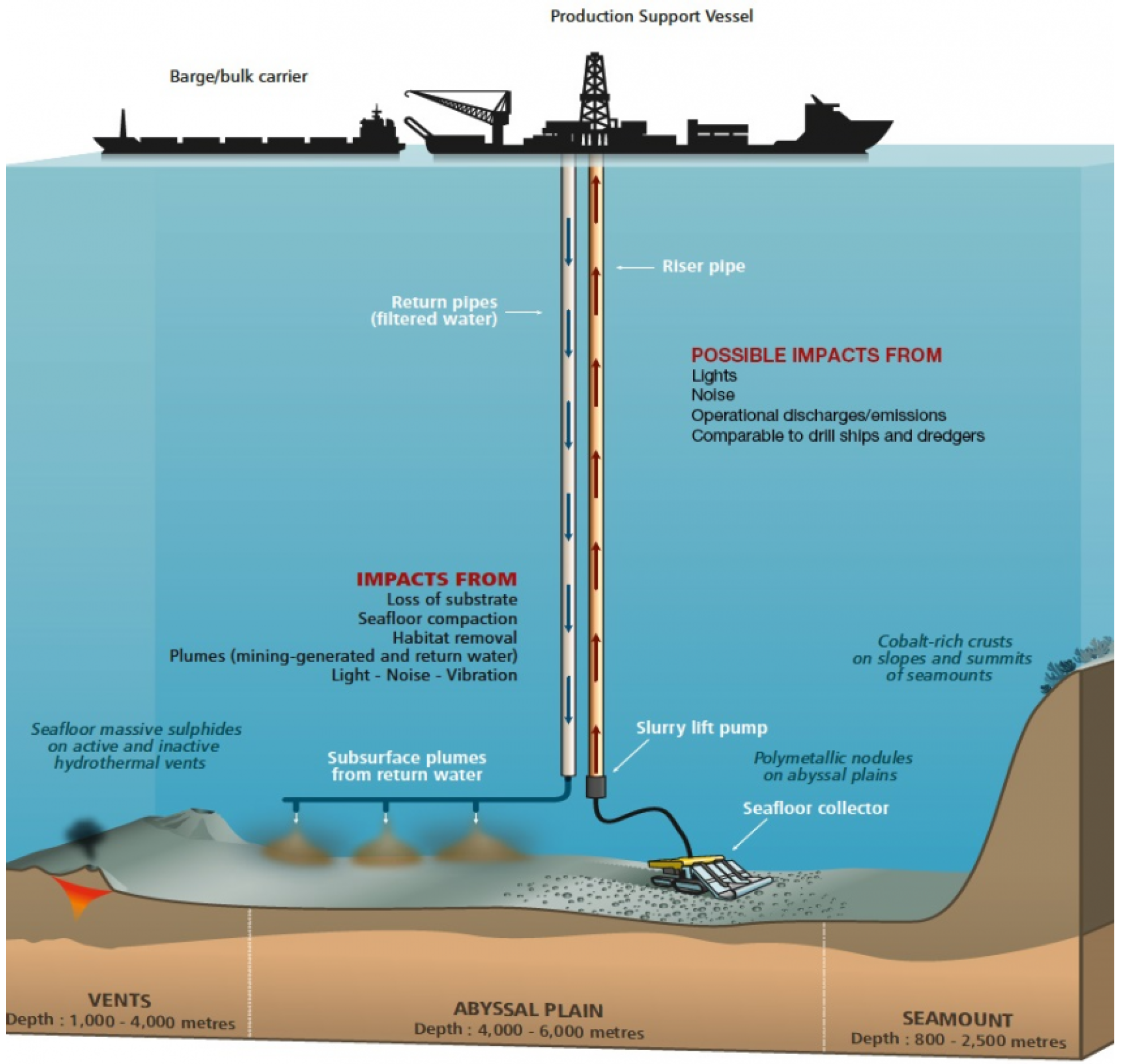
Table 1.
Estimated discharge conditions for various DSM cases for a PNMT.
| Application | Solid Flux Per Unit Width | Concentration Range | D10 | D50 | D90 |
|---|---|---|---|---|---|
| Seafloor Massive Sulfides (SMSs) [30] | 163 kg/s | 250 g/L | 19 μm | 40 μm | 70 μm |
| Nodules [6] | 65.9–212.3 kg/s | 10–170 g/L | - | 10 μm | - |
| Nodules [31] | 65.9–212.3 kg/s | 10–170 g/L | 2 μm | 15 μm | 70 μm |
| Fe-Mn crusts [17] | 0.2 kg/s | 20–100 mg/L | - | - | - |
| Phosphorite [32] | 827 kg/s | 449 g/L | 10 μm | 80 μm | 300 μm |
| Name of Sediment Fraction | Diameter Limits (Micro) WRB Classification | GSR Data Average (%) | NTNU Data BC062 (%) | NTNU Data BC064 (%) | IOM Data Average (%) |
|---|---|---|---|---|---|
| Clay | <2 | 12 | 11.3 | 14.5 | 23.24 |
| Silt | 2–63 | 76.2 | 85.7 | 82.5 | 70.36 |
| Sand | 63–2000 | 11.8 | 3 | 3 | 6.13 |
| IOM 1 | IOM 2 | IOM 3 | Site A | Site B | Site C | GSR | IOM | |
|---|---|---|---|---|---|---|---|---|
| Smectite (%) | 12.71 | 17.33 | 16.49 | 52 | 38 | 40 | 36.41 | 16.3 |
| Illite (%) | 13.82 | 12.05 | 14.25 | 31 | 42 | 50 | 48.34 | 13.2 |
| Kaolinite (%) | 0.65 | 0.43 | 0.54 | 10.33 | 1 | |||
| Chlorite (%) | 1.7 | 1.85 | 2.35 | 4.92 | 1.5 | |||
| Amorphic (%) | 50.47 | 47.09 | 44.42 |
Table 4.
Different entrainment coefficients values reported in the literature; “J” is the Jet-type flow. “P” is the Plume-type flow. “L” is Liquid. “P” is Pipe. “c” is Constriction. For the method, “w” is the hot wire probe and “l” is the laser Doppler anemometer. is the ratio in which z is the distance from the source. d is the discharge diameter [84].
| Source | Flow | Fluid | Nozzle | Method | Re | ||
|---|---|---|---|---|---|---|---|
| Forstall Gaylord (1955) | J | L | P | w | - | 10–20 | 0.070 |
| Wang Law (2002) | J | L | P | l | 12,700 | 40–80 | 0.075 |
| Papanicolaou List (1988) | J | L | c | l | 2460–10,900 | 40–50 | 0.074 |
| Papanicolaou List (1988) | J | L | c | l | 2460–10,900 | 50–80 | 0.079 |
| Papanicolaou List (1988) | P | L | c | l | 600 | 22–40 | 0.130 |
| Papanicolaou List (1988) | P | L | c | l | 600 | 41–53 | 0.126 |
| Papanicolaou List (1988) | P | L | c | l | 600 | 56–85 | 0.121 |
| Wang Law (2002) | P | L | c | l | 1550–12,700 | 31–55 | 0.124 |
Table 5.
Clay parameters used in the calculations of the erosion rate.
| D50 | ρp | PI | γcr | n | cv | cu |
|---|---|---|---|---|---|---|
| 0.012 mm | 1350 | 70% | 0.7 | 0.67 | m/s | 0.2 kPa |
Table 6.
Initial conditions of the numerical runs and the numerical results; , , , and are the results at the impingement point, while , , , and are the results 100 m downstream the impingement point.
Table 6.
Initial conditions of the numerical runs and the numerical results; , , , and are the results at the impingement point, while , , , and are the results 100 m downstream the impingement point.
| Runs | Initial Condition | Plume Model | Turbidity Current Model | |||||||||||
|---|---|---|---|---|---|---|---|---|---|---|---|---|---|---|
| 1 | 0 | 0.015 | 0.45 | 0.25 | 1.69 | - | - | - | - | 1.69 | 0.274 | 0.0067 | 0.91 | 1.672 |
| 2 | 0.02 | 0.34 | 0.25 | 1.69 | - | - | - | - | 1.69 | 0.274 | 0.0075 | 0.81 | 1.669 | |
| 3 | 0.025 | 0.27 | 0.25 | 1.69 | - | - | - | - | 1.69 | 0.274 | 0.0081 | 0.75 | 1.670 | |
| 4 | 0.5 | 0.015 | 0.45 | 0.25 | 1.69 | 0.97 | 0.009 | 0.62 | 0.22 | 1.22 | 0.235 | 0.0051 | 1.00 | 1.206 |
| 5 | 0.02 | 0.34 | 0.25 | 1.69 | 0.86 | 0.013 | 0.43 | 0.25 | 1.33 | 0.235 | 0.0051 | 1.00 | 1.206 | |
| 6 | 0.025 | 0.27 | 0.25 | 1.69 | 0.76 | 0.017 | 0.32 | 0.27 | 1.42 | 0.274 | 0.0059 | 0.91 | 1.322 | |
| 7 | 1.5 | 0.015 | 0.45 | 0.25 | 1.69 | 1.62 | 0.006 | 0.72 | 0.24 | 1.05 | 0.254 | 0.0065 | 0.85 | 1.398 |
| 8 | 0.02 | 0.34 | 0.25 | 1.69 | 1.42 | 0.010 | 0.44 | 0.30 | 1.27 | 0.220 | 0.0038 | 1.26 | 1.050 | |
| 9 | 0.025 | 0.27 | 0.25 | 1.69 | 1.29 | 0.013 | 0.32 | 0.35 | 1.44 | 0.244 | 0.0047 | 1.11 | 1.269 | |
| 10 | 0.015 | 0.45 | 0.5 | 1.69 | 3.48 | 0.010 | 0.61 | 0.43 | 2.48 | 0.257 | 0.0054 | 1.03 | 1.434 | |
| 11 | 0.02 | 0.34 | 0.5 | 1.69 | 3.05 | 0.013 | 0.43 | 0.47 | 2.67 | 0.323 | 0.0060 | 1.31 | 2.440 | |
| 12 | 0.025 | 0.27 | 0.5 | 1.69 | 2.73 | 0.017 | 0.32 | 0.52 | 2.83 | 0.332 | 0.0060 | 1.31 | 2.605 | |
Publisher’s Note: MDPI stays neutral with regard to jurisdictional claims in published maps and institutional affiliations. |
© 2021 by the authors. Licensee MDPI, Basel, Switzerland. This article is an open access article distributed under the terms and conditions of the Creative Commons Attribution (CC BY) license (https://creativecommons.org/licenses/by/4.0/).
Share and Cite
MDPI and ACS Style
Elerian, M.; Alhaddad, S.; Helmons, R.; van Rhee, C. Near-Field Analysis of Turbidity Flows Generated by Polymetallic Nodule Mining Tools. Mining 2021, 1, 251-278. https://doi.org/10.3390/mining1030017
AMA Style
Elerian M, Alhaddad S, Helmons R, van Rhee C. Near-Field Analysis of Turbidity Flows Generated by Polymetallic Nodule Mining Tools. Mining. 2021; 1(3):251-278. https://doi.org/10.3390/mining1030017
Chicago/Turabian StyleElerian, Mohamed, Said Alhaddad, Rudy Helmons, and Cees van Rhee. 2021. "Near-Field Analysis of Turbidity Flows Generated by Polymetallic Nodule Mining Tools" Mining 1, no. 3: 251-278. https://doi.org/10.3390/mining1030017