Defect Isolation from Whole to Local Field Separation in Complex Interferometry Fringe Patterns through Development of Weighted Least-Squares Algorithm

Abstract

In this paper, based on Gaussian 1σ-criterion and histogram segmentation, a weighted least-squares algorithm is applied and validated on digital holographic speckle pattern interferometric data to perform phase separation on the complex interference fields. The direct structural diagnosis tool is used to investigate defects and their impact on a complex antique wall painting of Giotto. The interferometry data is acquired with a portable off-axis interferometer set-up with a phase-shifted reference beam coupled with the object beam in front of the digital photosensitive medium. A digital holographic speckle pattern interferometry (DHSPI) system is used to register digital recordings of interferogram sequences over time. The surface is monitored for as long as it deforms prior to returning to its initial reference equilibrium state prior to excitation. The attempt to separate the whole vs. local defect complex amplitudes from the interferometric data is presented. The main aim is to achieve isolation and visualization of each defect’s impact amplitude in order to obtain detailed documentation of each defect and its structural impact on the surface for structural diagnosis purposes.

1. Introduction

Structural diagnosis in artworks refers to the detection of structural conditions and especially the documentation of structure abnormalities within the volume of the material and the threat that poses on the precious surface [1,2,3]. Understanding the structural condition and having detailed documentation of defects and their impact on the surface is the first and crucial step in every restoration plan [4,5,6,7,8,9]. Despite this essential step in culture restoration, the techniques used in structural diagnosis in everyday practices are still in infancy with the most advanced conservation practice being the subjective evaluation through touching and finger knocking on the precious surface, while qualitative X-ray radiography is the only advanced alternative [10]. The everyday practice is thus in both choices qualitative and fully dependent upon experience [11]. Shearography and terahertz techniques are used as intuitive deformation acquisition tools for complementary techniques in the field of heritage conservation [7], in which there is an urgent need for a rapid response and high-precision non-destructive testing method.

Digital holographic speckle pattern interferometry (DHSPI) provides a non-destructive non contacting remote operation portable prototype especially developed for cultural heritage applications, which signifies that the out-of-plane deformation common in expanding processes as artworks respond to the daily fluctuations of the environment. Coherent interferometry enables the structural diagnosis many advantages over the current practices as non-contact non-destructive full-field imaging with high resolution inherently quantitative data visualizing all sorts of different defects, in which they profile the depth from the surface to many tenths of a millimeter deep [12,13]. The plethora of advantages upgraded the method as the most promising one in cultural heritage structural diagnosis, creating a variety of techniques [14].

However rich the information content one can obtain from an interference image extracted from a surface revealing its sensitivity to environmental factors and invisible defects and defect impact to the surface, there is a main drawback in the data visualization creating problems in the unwrapping of defected surfaces and this referred to as fringe pattern complexity [15,16]. This is due to the high resolution of coherent interferometry rendering from one hand possible to investigate real artworks of complicated structural construction as the multi-layered mixed organic–inorganic objects are, including the most common artworks such as panel paintings, icons, wall paintings, frescoes, decorative items on furniture, etc., but from the other very dense complex interferograms due to plethora of defects. This is a very rich source of fringe pattern formation for detailed structural analysis and in-depth diagnosis but, on the other hand, creates a highly discontinuous interference field since the structural complex construction is affected more by the local complexity of the unavoidable presence of defects.

When such complex artworks are investigated for the detection of their defects the interferometric result can be very dense in terms of localized unique formation of interference fringes. The analysis requires a phase unwrapping on discontinuous interferograms. Therefore, the aim is to resolve the continuous interference fringes generated from the overall displacement of the whole body of the artwork; naturally or artificially, the very many distinct or interconnected fringe patterns of seemingly random appearance interrupt the otherwise expected smooth intensity distribution of the interference field.

Hence, in the structural diagnosis documentation context where each retrieved defect is to enter a defect map with exact coordinates for defect position, defect dimensions, shape and quantitative representation of the impact on the surface, then unwrapping becomes a tedious process which the unwrapping procedure itself alone fail to deliver or depict clearly. The unwrapping thus becomes a less adequate method for complex interferograms in cultural heritage diagnosis and this drawback needs correction. In order to make unwrapping more valuable in the artwork documentation problem, a method to separate the displacement due to the overall movement of the object that is the interference whole field from the local distinct defect pattern emerging from the whole field interrupting it, we need additional mathematical tools to add to the unwrapping procedure.

To this aim, we present here a phase separation method that can help advance the solution of complex defect patterns and there is evidence of the possibility to perform this procedure routinely as a variety of data tested prove and validate the method. This method is based on Gaussian 1σ-criterion and histogram segmentation, and we propose a weighted least-squares algorithm [17] to separate the deformation of the whole body vs. the local body. In this paper on this very important problem for the automatic recognition of defects, we use complex interferometry data from real artworks to show that complex interferograms are accessible to detailed documentation and quantitative evaluation, by separating the whole field and examining the local field representing each defect and its impact.

2. Experimental Methodology

2.1. Phase Separation Method of Whole Field vs. Local Field

Due to the arctangent operation, the value range of phase difference with regard to the deformation is between $(-\pi ,\pi )$, which is generally in the form of fringe patterns. A common method for quantifying defects directly with fringe patterns is to count the fringes of the interferogram with line profiles on both the x and y axes. However, the interferometric result of the investigated complex artworks can be very dense in terms of localized uniquely shaped interference fringes. Therefore, we propose a phase separation method based on a weighted least-squares algorithm to isolate the phase of the local body (or defect region) for accurate quantification.

Since thermal or other excitation-induced method waves reach the surface of the mural in the form of spherical waves, they will excite both the local body and the whole body at the same time. We unwrap the obtained fringe patterns as

$$\mathsf{\Phi }(x,y)=UNWRAP\left[\Delta \varphi (x,y)\right]\approx {\mathsf{\Phi }}_w(x,y)+{\mathsf{\Phi }}_l(x,y),$$

(1)

where $\Delta \varphi (x,y)$ represents the phase difference (i.e., fringe pattern) with regard to deformation, UNWRAP[·] indicates the phase unwrapping operation, ${\mathsf{\Phi }}_w(x,y)$ and ${\mathsf{\Phi }}_l(x,y)$ represents the whole-body phase and local-body region phase, respectively.

Assuming that the whole body of the mural is isotropic in a uniformly distributed laminated structure, based on the spherical waveform characteristics of acoustic excitation, we accept that the deformation of the whole body can be manifested as a quadratic term phase. Thus, ${\mathsf{\Phi }}_w(x,y)$ can be written as

$${\mathsf{\Phi }}_w(x,y)\approx u_1+u_{2}x+u_{3}y+u_{4}xy+u_5{x}^2+u_6{y}^2,$$

(2)

where $x=x_1,x_2,\dots ,x_N;y=y_1,y_2,\dots ,y_M;N,M\in \mathbb{Z}$.

Equation (2) expresses an overdetermined equation [17,18,19,20]. The overdetermined system in the traditional least-squares algorithm [21] can be expressed as

$$\left[\begin{array}{cccccc}1& x_1& y_1& x_1{y}_1& x_1^2& y_1^2\\ 1& x_2& y_2& x_2{y}_2& x_2^2& y_2^2\\ ⋮& ⋮& ⋮& ⋮& ⋮& ⋮\\ 1& x_n& y_n& x_n{y}_n& x_n^2& y_n^2\end{array}\right]\left[\begin{array}{c}{u}_1\\ u_2\\ u_3\\ u_4\\ u_5\\ u_6\end{array}\right]=\left[\begin{array}{c}\varphi (x_1,y_1)\\ \varphi (x_2,y_2)\\ ⋮\\ \varphi (x_n,y_n)\end{array}\right],$$

(3)

where $\varphi (x,y)$ represents any phase information.

The above roughly corrected phase is divided into 10 × 10 grids, and then the maximum–minimum–average–standard deviation (MMASD) evaluation metric is used for pre-compensation, from which the weighted matrix $\omega (x,y)$ can be obtained by the threshold segmentation based on the Gaussian 1σ-criterion [17].

By introducing the weighted least-squares algorithm, based on Equation (3) accurate quadratic term coefficients would be obtained as

$${\mathit{U}}_{\omega }={\left[\mathit{S}{(x,y)}^T\cdot \mathit{S}(x,y)\cdot \omega (x,y)\right]}^{-1}\cdot \left[\mathit{S}{(x,y)}^T\cdot \varphi (x,y)\cdot \omega (x,y)\right],$$

(4)

where $\mathit{S}(x,y)=\left[\begin{array}{cccccc}1& x& y& xy& x^2& y^2\end{array}\right]$ represents the matrix of the polynomials in Equation (3), ${\mathit{U}}_{\omega }={\left[\begin{array}{cccccc}{u}_1& u_2& u_3& u_4& u_5& u_6\end{array}\right]}^T$ represents the vector of quadratic estimation coefficients, where the superscript T represents the transpose of a matrix or vector.

Therefore, the above quadratic term phase information ${\mathsf{\Phi }}_w(x,y)$ can be eliminated, and thus, ${\mathsf{\Phi }}_l(x,y)$ can be separated from $\mathsf{\Phi }(x,y)$ as

$${\mathsf{\Phi }}_l(x,y)\approx \mathsf{\Phi }(x,y)-\mathit{S}(x,y)\cdot {\mathit{U}}_{\omega },$$

(5)

Based on an object-beam reflection-based optical setup, the strain distribution of the defect can be derived to achieve accurate quantification. Therefore, we can obtain the deformation $\delta (x,y)$ of the local body by

$$\delta (x,y)\approx \frac{\lambda {\mathsf{\Phi }}_l(x,y)}{4\pi }$$

(6)

where $\lambda$ = 532 nm represents the wavelength of the laser.

As shown in Figure 1, the whole field vs. local field phase can be separated using the proposed phase separation method. Figure 1(a₁,a₂) show the fringe patterns and the corresponding unwrapped phase, respectively. Folds appear at the densest fringes in Figure 1(a₁), and, as mentioned earlier, too-dense fringes interfere with the quantification of defects. The unwrapped phase presents the spherical wave characteristics of the quadratic term. Based on the weighted least-squares algorithm, the 10 × 10 grid phase of Figure 1(b₁) and the weighted matrix $\omega (x,y)$ of Figure 1(b₂) are obtained sequentially. Using Equation (5), the phases of the whole body and the local body are separated, as shown in Figure 1(c₁,d₁), respectively. Figure 1(c₁,c₂) exhibit the same phase characteristics as that of Figure 1(a₁,a₂), which demonstrates the effectiveness of our method in separating the whole field phase. From Equation (6), Figure 1(d₁,d₂) show the phase and strain distribution of the local body, respectively. The local-body phase is on a relatively flat plane, and the abnormal strain can be clearly displayed in the above phase distribution. The strain distribution of the defect in Figure 1(d₂) is in the micron level, which is beyond the range of $\lambda$/2, indicating that interfering fringes can occur in the fringe pattern. The proposed method achieves the “fringe-pattern-free” of the local-body phase, which shows that our method can also eliminate the above-mentioned interfering fringes.

2.2. System View

In DHSPI, the interferometric comparison is achieved by two beams of the same laser after amplitude-modulated beam splitting providing the two arms of an interferometer, from which one is mirror driven and the collimator expanded to illuminate by a controlled divergence beam the surface. As shown in Figure 2a,b, the light source is a continuous wave solid state at 532 nm, the digital recording component consists of a CMOS camera of 5 Mp, and a PZT crystal for the phase shifting [22]. The beam illuminating the object is termed Object Beam and the other, spatially filtered and collimated, that is used to serve as a reference for the interference phenomenon to take place is termed Reference Beam. As a result, interference is produced and collected on a CMOS plane to be acquired by a frame grabber and further analyzed by numerical processes via specially developed software. Schematic representation of the DHSPI optical geometry satisfying fundamental holographic interferometry operation principle. The collected interferometric data provides hundreds of images depending on the initial excitation and the conservation state of the examined artwork [13]. The complex interferometry field is combined by the displacement due to the induced excitation and the impact of subsurface defects that are displaced with their own dynamic. The result is a simple or complex interference field of surface displacement and defect, which is generally displayed in the form of fringe patterns.

For provoking the optical displacement of the surface to visualize the impact of defects on the surface in order to perform a standardized protocol of defect documentation, two infrared lamps of 175 W are used as excitation sources. The reference state of the surface is registered prior to induced displacement and the sequential acquisition step starts after the surface has been displaced. The focal length of the convex lens is 25 mm to provide a field of view of 30 cm × 30 cm, with the size of the pixel being 3.45 μm × 3.45 μm. The deduction magnification of CCD imaging is about 40×. Therefore, the lateral resolution of the system for defect detection is about 3.45 μm × 40 = 138 μm. In the reflective deformation measurement of DH [23], according to the minimum grayscale value subtracted from the two adjacent holograms detected by CCD, the axial resolution of the system for defect detection is 532/(2 × 256) ≈ 1 nm.

3. Experimental Results

3.1. Comparison of Quantitative Methods

The fringe patterns provide a direct visual tool to identify local-faulted bodies of structural discontinuity in regards to the overall surface displacement from its initial position. Deformation occurs as a result of instantaneous or continuous or gradual displacement processes that influence the physicmechanical integrity or physicochemical composition of materials deteriorating the constitution and construction of objects [15,24].

Deformation occurs as a result of instantaneous or continuous or gradual displacement processes that influence the physicmechanical integrity or physicochemical composition of materials deteriorating the constitution and construction of objects [25]. The traditional defects quantification method is the direct analysis of the fringe patterns and the unwrapped phase, which is prone to blurring and low-precision results. In the fringe patterns, the whole-body phase dominates in the graphical representation, which would mask minor abnormalities in the local body. Based on the phase separation method, the above graphical representation of the whole-body phase can be effectively removed; thus, the phase distribution of the local body will be separated for quantitative analysis, followed by the strain distribution of the local bodies obtained based on Equation (6).

Figure 3 illustrates and compares three types of phase information for identifying surface and subsurface defects: the wrapped phase (i.e., fringe patterns) in Figure 3b, the unwrapped phase in Figure 3c, and the isolated local-body phase using our method in Figure 3f. Figure 3a,b are the original photos of the sampling fresco area and the obtained fringe patterns map, respectively. The red dashed lines in Figure 3b circle the identification of pattern classifications in the fringe patterns. Figure 3b shows five typical fringe species: circular fringes; curved fringes; density changed fringes; direction-changed fringes; and dead-end fringes. The fringe pattern classification to defect identification is verified through experimental and mathematical verification and is validated through “known-defect” applications which is the term indicating a reverse engineering verification approach through the use of purposefully induced defects in technical samples. Figure 3c shows the unwrapped phase map of the above fringe pattern. Using Equations (5) and (6), the phases of the whole body and the strain distribution of the local body are separated, as shown in Figure 3d,f, respectively. Figure 3d,e exhibit the same phase characteristics as that of Figure 3b,c, which demonstrates the effectiveness of our method in separating the whole field phase. The blue dashed line in Figure 3f marks the range of strain anomalies in the sampling area. Redrawing the red dashed line of Figure 3b and the blue dashed area of Figure 3f into Figure 3a, respectively, we can see that there is an overlap between the red dashed and blue dashed areas, illustrating the consistency of our method with the fringe identification method. At the same time, our method can obtain more accurate lateral and axial detection ranges, indicating the high accuracy of the phase separation method.

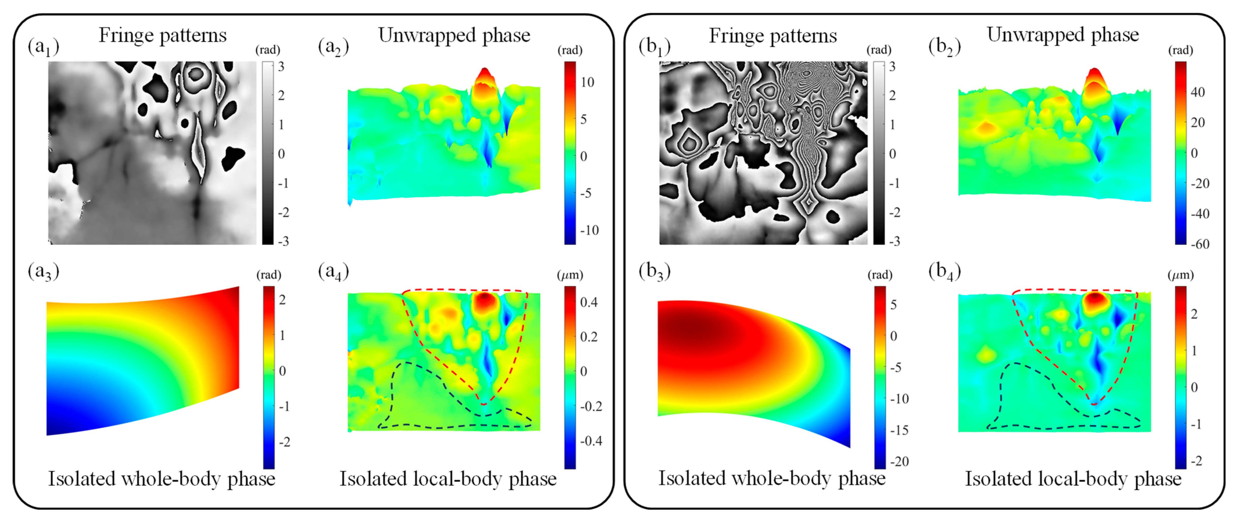
3.2. Contrast Treatment of Simple and Complex Fringe Patterns

Fringe pattern classification is especially useful for qualitative defect diagnosis as a direct on-field diagnosis method. In the fringe pattern, the whole-body phase dominates in the graphical representation, which might mask minor abnormalities in the local body. Based on the phase separation method, the above graphical representation of the whole-body phase can be effectively removed, thus the phase distribution of the local body will be separated for quantitative analysis.

Figure 4(a₁–a₄,b₁–b₄) show the fringe patterns, unwrapped phase, separated whole-body phase and the corresponding local-body strain distributions of single and complex fringes, respectively. Figure 4(a₁,b₁) show fringe patterns acquired in the same sampling area, showing low-density and high-density fringe patterns due to different excitation times. Obviously, the fringe identification table in Section 3.1 obtains less defect qualitative information for low-density fringe patterns. The unwrapped phase maps of Figure 4(a₂,b₂) are skewed, which can be misleading to actual defect quantification. Figure 4(a₃,b₃) separate the whole-body phase maps and verify the tilt and spherical aberration described above. For the effectiveness of phase separation, we have a visual demonstration of the separation effect. According to our hypothesis, the whole-body phase and the local-body phase have different phase characteristics. As shown in Figure 4(a₃,b₃), the whole-body phase is similar to the spherical wave, has the characteristics of quadratic term aberration, and carries the polynomial coefficients of the radius of curvature and the angle of inclination, as noted in Equation (2). As shown in Figure 4(a₄,b₄), the local-body phase is characterized by an up-and-down phase or strain change in the defect region on a relatively flat plane. The black dashed line indicates a relatively flat area, while the red dashed line indicates the strain distribution in the defect area. The strain distribution of the local body of Figure 4(a₄,b₄) has great similarity in the transverse direction, indicating the effectiveness of the proposed method. At the same time, due to the difference in excitation time, the local-body phase of simple fringes and complex fringes has numerical differences in the axial direction, indicating that the defect parts are susceptible to excitation and have a cumulative effect.

3.3. Mural Cooling Process

The reflected photons statistically interfere with neighboring photons involved in the same path and change to produce displacement of the same phase change value, which gives rise to interference fringes extended in the surface for as far as the phase value remains the same. Non-destructive thermal excitation refers to achieving about 2 °C (such as 21.5–23.5 °C) in a short period of time, followed by a slow cooling-down duration. We chose the cooling process of the mural and obtained the fringe pattern within 567 s of cooling. Figure 5 shows the fringe patterns, unwrapped phase map, the separated whole-body phase map and local-body strain distribution from the cooling process of 6 groups, respectively. Observing the fringe patterns of Figure 5a–f, it can be seen that the fringe density gradually decreases with the increase in cooling time. However, in Figure 5e,f, fringe density is hard to be used as a direct quantitative criterion. The unwrapped phase maps of Figure 5a–f have different degrees of skew and spherical aberration. The unwrapped phase maps of Figure 5e,f cannot distinguish the location of the defects as that in Figure 5a–d, which means that the qualitative analysis of defects using the unwrapped phase map fails.

Figure 5a–f show the separated whole-body phases, and it can be observed that as the cooling time increases, the center of the spherical difference varies. As can be observed from the local-body strain distributions of Figure 5a–f, the proposed method can robustly obtain the position and shape of the defect and even perform precise quantification at each stage with the cooling time.

4. Conclusions

In this study, a phase separation method based on the weighted least-squares algorithm is applied and validated to conveniently isolate the local phase distribution from the whole, complex fringe pattern. This method is examined to accurately quantify the deformation distribution of defects in simple and complex fringes. In experimental work, the DHSPI system is used to register digital recordings of interferogram sequences over time. The proposed method enables highly accurate quantitative post-processing analysis for investigating defects and their impact on a complex antique wall painting of Giotto. Results show that the suggested phase separation method allows isolation and visualization of each defect’s impact amplitude as well as quantified surface deformation providing a detailed documentation of each defect and its structural impact on the surface for structural diagnosis purposes to the conservators. Since 3D digitization is of great significance to the protection and display of CH [26,27], in future work, we will combine 3D digitization to estimate and reconstruct internal defects.

References

1. Anaf, W.; Cabal, A.; Robbe, M.; Schalm, O. Real-Time Wood Behaviour: The Use of Strain Gauges for Preventive Conservation Applications. Sensors 2020, 20, 305. [Google Scholar] [CrossRef] [PubMed]
2. Tiennot, M.; Iannuzzi, D.; Hermens, E. Evolution of the Viscoelastic Properties of Painting Stratigraphies: A Moisture Weathering and Nanoindentation Approach. Herit. Sci. 2021, 9, 77. [Google Scholar] [CrossRef]
3. Gülker, G.; Hinsch, K.D.; Kraft, A. TV-Holography on a Microscopic Scale: Deformation Monitoring on Polychrome Terracotta Warriors. In Interferometry in Speckle Light; Jacquot, P., Fournier, J.-M., Eds.; Springer: Berlin/Heidelberg, Germany, 2000; pp. 337–344. ISBN 978-3-642-63230-3. [Google Scholar]
4. Buchta, D.; Heinemann, C.; Pedrini, G.; Krekel, C.; Osten, W. Combination of FEM Simulations and Shearography for Defect Detection on Artwork. Strain 2018, 54, e12269. [Google Scholar] [CrossRef]
5. Zhao, Q.; Dan, X.; Sun, F.; Wang, Y.; Wu, S.; Yang, L. Digital Shearography for NDT: Phase Measurement Technique and Recent Developments. Appl. Sci. 2018, 8, 2662. [Google Scholar] [CrossRef]
6. Picollo, M.; Fukunaga, K.; Labaune, J. Obtaining Noninvasive Stratigraphic Details of Panel Paintings Using Terahertz Time Domain Spectroscopy Imaging System. J. Cult. Herit. 2015, 16, 73–80. [Google Scholar] [CrossRef]
7. Groves, R.M.; Pradarutti, B.; Kouloumpi, E.; Osten, W.; Notni, G. 2D and 3D Non-Destructive Evaluation of a Wooden Panel Painting Using Shearography and Terahertz Imaging. NDT E Int. 2009, 42, 543–549. [Google Scholar] [CrossRef]
8. Van der Maaten, L.; Erdmann, R.G. Automatic Thread-Level Canvas Analysis: A Machine-Learning Approach to Analyzing the Canvas of Paintings. IEEE Signal Process. Mag. 2015, 32, 38–45. [Google Scholar] [CrossRef]
9. Baxter, J. Quasi-Reflectography. Nat. Photon 2012, 6, 572. [Google Scholar] [CrossRef]
10. Eveno, M.; Moignard, B.; Castaing, J. Portable Apparatus for In Situ X-Ray Diffraction and Fluorescence Analyses of Artworks. Microsc. Microanal. 2011, 17, 667–673. [Google Scholar] [CrossRef]
11. Daher, C.; Paris, C.; Le Hô, A.-S.; Bellot-Gurlet, L.; Échard, J.-P. A Joint Use of Raman and Infrared Spectroscopies for the Identification of Natural Organic Media Used in Ancient Varnishes: Spectroscopic Identification of Natural Organic Media Used in Ancient Varnishes. J. Raman Spectrosc. 2010, 41, 1494–1499. [Google Scholar] [CrossRef]
12. Georges, M.P.; Scauflaire, V.S.; Lemaire, P.C. Compact and Portable Holographic Camera Using Photorefractive Crystals. Application in Various Metrological Problems. Appl. Phys. B 2001, 72, 761–765. [Google Scholar] [CrossRef]
13. Memmolo, P.; Arena, G.; Fatigati, G.; Grilli, M.; Paturzo, M.; Pezzati, L.; Ferraro, P. Automatic Frames Extraction and Visualization From Noisy Fringe Sequences for Data Recovering in a Portable Digital Speckle Pattern Interferometer for NDI. J. Disp. Technol. 2015, 11, 417–422. [Google Scholar] [CrossRef]
14. Kang, Y.-J.; Baik, S.-H.; Ryu, W.-J.; Kim, K.-S. Measurement of Shock Waves Using Phase Shifting Pulsed Holographic Interferometer. Opt. Laser Technol. 2003, 35, 323–329. [Google Scholar] [CrossRef]
15. Osten, W.; Jueptner, W.P.O.; Mieth, U. Knowledge-Assisted Evaluation of Fringe Patterns for Automatic Fault Detection; Pryputniewicz, R.J., Brown, G.M., Jueptner, W.P.O., Eds.; Springer: San Diego, CA, USA, 1994; pp. 256–268. [Google Scholar]
16. Ding, L.; Wan, H.; Lu, Q.; Chen, Z.; Jia, K.; Ge, J.; Yan, X.; Xu, X.; Ma, G.; Chen, X.; et al. Using Deep Learning to Identify the Depth of Metal Surface Defects with Narrowband SAW Signals. Opt. Laser Technol. 2023, 157, 108758. [Google Scholar] [CrossRef]
17. Chen, Z.; Zhou, W.; Duan, L.; Zhang, H.; Zheng, H.; Xia, X.; Yu, Y.; Poon, T. Automatic Elimination of Phase Aberrations in Digital Holography Based on Gaussian 1σ- Criterion and Histogram Segmentation. Opt. Express 2023, 31, 13627. [Google Scholar] [CrossRef]
18. Di, J.; Zhao, J.; Sun, W.; Jiang, H.; Yan, X. Phase Aberration Compensation of Digital Holographic Microscopy Based on Least Squares Surface Fitting. Opt. Commun. 2009, 282, 3873–3877. [Google Scholar] [CrossRef]
19. Liu, S.; Xiao, W.; Pan, F. Automatic Compensation of Phase Aberrations in Digital Holographic Microscopy for Living Cells Investigation by Using Spectral Energy Analysis. Opt. Laser Technol. 2014, 57, 169–174. [Google Scholar] [CrossRef]
20. Liu, S.; Liu, Z.; Xu, Z.; Han, Y.; Liu, F. Automatic and Accurate Compensation for Phase Aberrations in Digital Holographic Microscopy Based on Iteratively Reweighted Least Squares Fitting. Opt. Laser Technol. 2023, 167, 109704. [Google Scholar] [CrossRef]
21. Ren, Z.; Zhao, J.; Lam, E.Y. Automatic Compensation of Phase Aberrations in Digital Holographic Microscopy Based on Sparse Optimization. APL Photonics 2019, 4, 110808. [Google Scholar] [CrossRef]
22. Tornari, V.; Tsigarida, A.; Ziampaka, V.; Kousiaki, F.; Kouloumpi, E. Interference Fringe Patterns in Documentation on Works of Art: Application on Structural Diagnosis of a Fresco Painting. Am. J. Art. Des. 2017, 2, 1–15. [Google Scholar] [CrossRef]
23. Roye, W.; Crostack, H.-A. Profile- and Deformation-Measurements with High Axial Resolution Using the Acoustical Holography. Nucl. Eng. Des. 1987, 102, 313–317. [Google Scholar] [CrossRef]
24. Rippa, M.; Pagliarulo, V.; Lanzillo, A.; Grilli, M.; Fatigati, G.; Rossi, P.; Cennamo, P.; Trojsi, G.; Ferraro, P.; Mormile, P. Active Thermography for Non-Invasive Inspection of an Artwork on Poplar Panel: Novel Approach Using Principal Component Thermography and Absolute Thermal Contrast. J. Nondestruct. Eval. 2021, 40, 21. [Google Scholar] [CrossRef]
25. Daffara, C.; Ambrosini, D.; Pezzati, L.; Paoletti, D. Thermal Quasi-Reflectography: A New Imaging Tool in Art Conservation. Opt. Express 2012, 20, 14746. [Google Scholar] [CrossRef]
26. Wang, D.; Li, N.-N.; Li, Y.-L.; Zheng, Y.-W.; Nie, Z.-Q.; Li, Z.-S.; Chu, F.; Wang, Q.-H. Large Viewing Angle Holographic 3D Display System Based on Maximum Diffraction Modulation. Light Adv. Manuf. 2023, 4, 1. [Google Scholar] [CrossRef]
27. Wang, D.; Li, Z.-S.; Zheng, Y.-W.; Li, N.-N.; Li, Y.-L.; Wang, Q.-H. High-Quality Holographic 3D Display System Based on Virtual Splicing of Spatial Light Modulator. ACS Photonics 2023, 10, 2297–2307. [Google Scholar] [CrossRef]
Figure 1. The process of phase separation method with the experimental data: (a1,a2) are wrapped phase and the corresponding unwrapped phase, respectively; (b1,b2) are the grid phase and weighted matrix ω ( x , y ) , respectively; (c1,c2) are re-wrapped phase map and the 3D rendering of the separated whole-body phase distribution, respectively; (d1,d2) are the isolated local-body phase distribution and the corresponding 3D rendering, respectively.
Digital 04 00004 g001
Figure 2. (a) DHSPI portable system scheme and (b) system on scaffold investigating Giotto layers.
Digital 04 00004 g002
Figure 3. A comparison of the method with the traditional identification method: (a) original photo of the sampling fresco area; (b) obtained fringe patterns map; (c) unwrapped phase map; (d) separated whole-body phase map; (e) re-wrapped phase map of (d); (f) isolated local-body phase map.
Digital 04 00004 g003
Figure 4. Simple fringe vs. complex fringe: (a1a4) are the fringe patterns, unwrapped phase, separated whole-body phase and the corresponding local-body strain distribution of simple fringes, respectively; (b1b4) are the fringe patterns, unwrapped phase, separated whole-body phase and the corresponding local-body strain distribution of complex fringes, respectively.
Digital 04 00004 g004
Figure 5. Cooling process of the mural: (a) obtained fringe patterns, unwrapped phase, separated whole-body phase and local-body strain distribution of 6 s; (b) obtained fringe patterns, unwrapped phase, separated whole-body phase and local-body strain distribution of 102 s; (c) obtained fringe patterns, unwrapped phase, separated whole-body phase and local-body strain distribution of 228 s; (d) obtained fringe patterns, unwrapped phase, separated whole-body phase and local-body strain distribution of 324 s; (e) obtained fringe patterns, unwrapped phase, separated whole-body phase and local-body strain distribution of 432 s; (f) obtained fringe patterns, unwrapped phase, separated whole-body phase and local-body strain distribution of 540 s.
Digital 04 00004 g005
Disclaimer/Publisher’s Note: The statements, opinions and data contained in all publications are solely those of the individual author(s) and contributor(s) and not of MDPI and/or the editor(s). MDPI and/or the editor(s) disclaim responsibility for any injury to people or property resulting from any ideas, methods, instructions or products referred to in the content.