Towards a Machine Learning Snowfall Retrieval Algorithm for GPM-IMERG ^†

Abstract

Remote sensing of snowfall has been proved to be a great challenge since the start of the satellite era. Several techniques have been applied to satellite data to estimate the fraction of frozen precipitation that reaches the surface. This study aims at investigating the efficacy of machine learning (ML), and especially deep learning (DL), in estimating the precipitation phase of the Integrated Multi-satellitE Retrievals for the Global Precipitation Measurement (GPM-IMERG). To achieve this, a training phase with hourly high-resolution numerical model outputs and in situ data was chosen for the period of late-2020 and 2021. Preliminary results show that ML models can estimate the precipitation phase with relatively high accuracy based on several case studies. The findings suggest that ML models offer a promising approach for advancing the nowcasting of snowfall and building a long-term archive dataset of IMERG-based snowfall using conventional real-time data.

1. Introduction

Deriving the phase of precipitation and distinguishing between its liquid and frozen state is of major importance for human activities, hydrological processes, and climate change studies [1,2]. For example, in a drainage basin the response time is different for rainfall and snowfall, while for remotely sensed observations a misclassification of precipitation phase can result in significant errors in the estimated precipitation rate [2,3]. Towards this direction, a plethora of techniques is being used today to detect snowfall. Some of the most successful methods include using measurements from in situ instruments, remote sensing through dual-wavelength radars, or using gridded data from numerical weather models [4,5]. However, none of those approaches has been proved fully reliable, while for the most accurate ones, such as the measurements from in situ instruments, the available data are generally sparse or even absent, for example in mountainous or sparsely populated areas [2,6]. The use of satellite data to obtain precipitation estimates has been one of the most used methods for measuring precipitation so far, giving both satisfactory and continuous results with almost no missing values or temporal and spatial gaps [7]. Nonetheless, the estimation of the precipitation phase based solely on satellites is still of mediocre performance for various reasons [8].

Machine learning is a subset of artificial intelligence that uses algorithms which can learn a model or a set of rules from an existing labeled dataset, with the goal of correctly predicting new and unlabeled data [9]. The use of machine learning in meteorology has been constantly increasing during the last few years, and is predicted to increase even more, as more and more data that can be used to train those models become available [10]. The problem of determining precipitation phase has been studied before, both with conventional and machine learning methods [2,6,11,12]. In this study, machine learning and especially deep learning algorithms are used along with numerical weather data and in situ observational data to classify the phase of precipitation acquired by the Integrated Multi-satellitE Retrievals for the Global Precipitation Measurement (GPM-IMERG) operated by the National Aeronautics and Space Administration (NASA) [13].

2. Materials and Methods

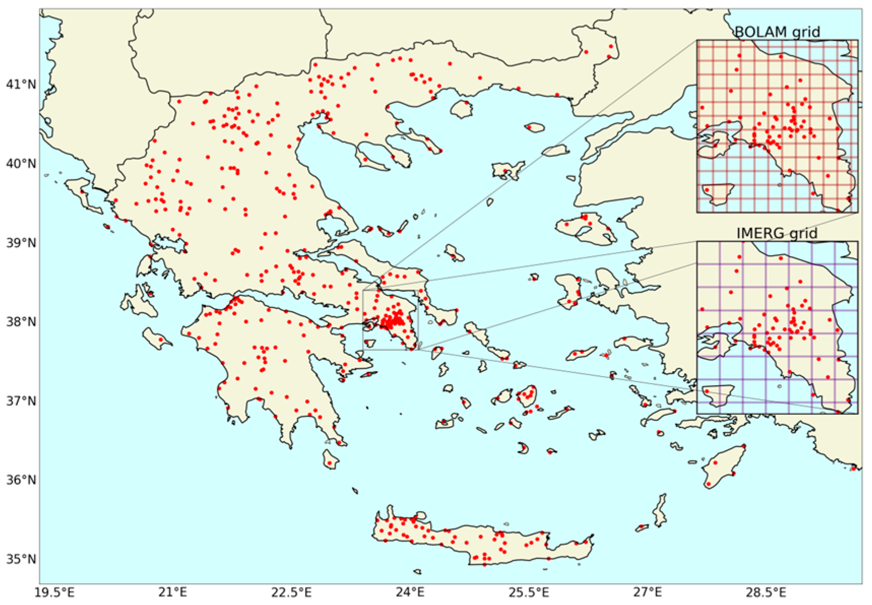
2.1. Description of the Acquired Data

During the past 15 years, the Institute for Environmental Research and Sustainable Development of the National Observatory of Athens (NOA/METEO) has established and is currently managing a dense network of automated weather stations throughout Greece (NOAAN) [14]. The in situ variables used in this study include the air temperature, relative humidity, and atmospheric pressure from the weather stations depicted in Figure 1.

The National Observatory of Athens runs the hydrostatic meteorological Bologna Limited-Area Model (BOLAM) in operational mode. The current set-up of BOLAM at NOA/METEO involves a grid covering Europe, the Mediterranean basin, and North Africa. The grid consists of 770 × 702 points with a 0.06° horizontal grid interval (~6 km) and 40 vertical levels [15].

The Integrated Multi-satellitE Retrievals for GPM (IMERG) algorithm is designed to intercalibrate, combine, and interpolate microwave precipitation measurements, along with microwave-calibrated infrared (IR) satellite measurements, precipitation gauge analyses, and possibly other precipitation estimators at fine time and space scales worldwide. The system runs multiple times for each observation time, providing a first estimation and successively generating more accurate estimates as more data become available. IMERG covers a global grid with a spatial resolution of 0.1° and its early products are available with a delay of approximately 4 h, in 30 min time intervals [13]. The precipitation phase in IMERG is currently computed diagnostically, based on the Liu scheme [2]. The Liu scheme used by NASA calculates the probability of liquid precipitation based solely on data from a numerical weather model or model analysis, relying on surface wet-bulb temperature (Tw) values [2,5].

2.2. Creation of a Custom Dataset

Snowfall observations in Greece are sparse in time and space, and usually only available in airports, where staff are present (e.g., [16]). Thus, these data are not enough to train a machine learning model and a different approach should be considered. Sims and Liu (2015) [2] showed that Tw is a better indicator than ambient air temperature for separating solid and liquid precipitation. Since air temperature, relative humidity, and atmospheric pressure data are available from the dense NOAAN weather station network, a dataset classifying whether favorable conditions for snowfall were present for each station observation can be created, based on Tw.

Using NOAAN observations for air temperature, relative humidity and atmospheric pressure, BOLAM’s nowcast (first 12 h after model initialization time) and the 1.1 °C Tw threshold chosen by NASA for IMERG V06 over land as the value corresponding to a probability of liquid precipitation equal to 50%, a new dataset is created [5]. For each in situ observation, the new dataset contains information about whether snowfall conditions were favorable according to the Tw < 1.1 °C threshold, the corresponding numerical weather model data for the nearest grid point, as well as the station metadata such as latitude, longitude, and altitude. This dataset contains data for 480 locations in Greece with a temporal resolution of 30 min for late-2020 and 2021.

2.3. Machine Learning Models Used

Our goal is to train machine learning models that, given only the numerical weather model’s data and metadata for a specific location, are able to solve the classification task of predicting whether favorable conditions for snow are present near the surface or not. This layer can then be used as a mask on IMERG precipitation products to create an IMERG-Snow dataset.

Machine learning models are trained on a training dataset and then tested on a testing dataset that contains data the models have never encountered before. Building training and testing datasets can be a challenging task, since weather data can overlap in space and time, thus making the testing dataset not completely intact. For the purpose of this study, spatial independence is achieved by building training and testing datasets that do not contain data from identical station locations.

The two types of machine learning models used to solve this classification problem are gradient boosting and feedforward neural networks. The latter are a subset of deep learning, where multiple layers are used to extract information from data.

Gradient boosting is a popular machine learning technique used, among others, in classification tasks. It works by creating multiple weak models, which often are decision trees, and combining them to form a better performing model. This is usually undertaken by building an initial weak model, then a second model aiming to more accurately predict the cases where the first one performs poorly, etc. Each new model created targets minimizing the error of the loss function; thus, the gradient of the loss function is calculated in every step of the algorithm [17].

Feedforward neural networks are the simplest type of artificial neural networks, where information moves only in a forward direction, from the input nodes, to the hidden nodes and to the output nodes. Here, a multilayer neural network, also called a multilayer perceptron, is used. A multilayer perceptron consists of multiple layers of computational units, containing neurons that are connected to the neurons of the next layer. These models are trained using back-propagation, a technique utilized to adjust the weight values of each connection in a way that minimizes the error between predictions and actual values [18,19].

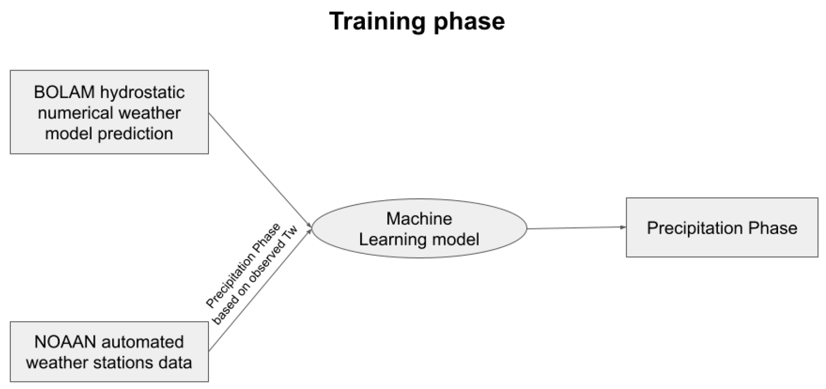
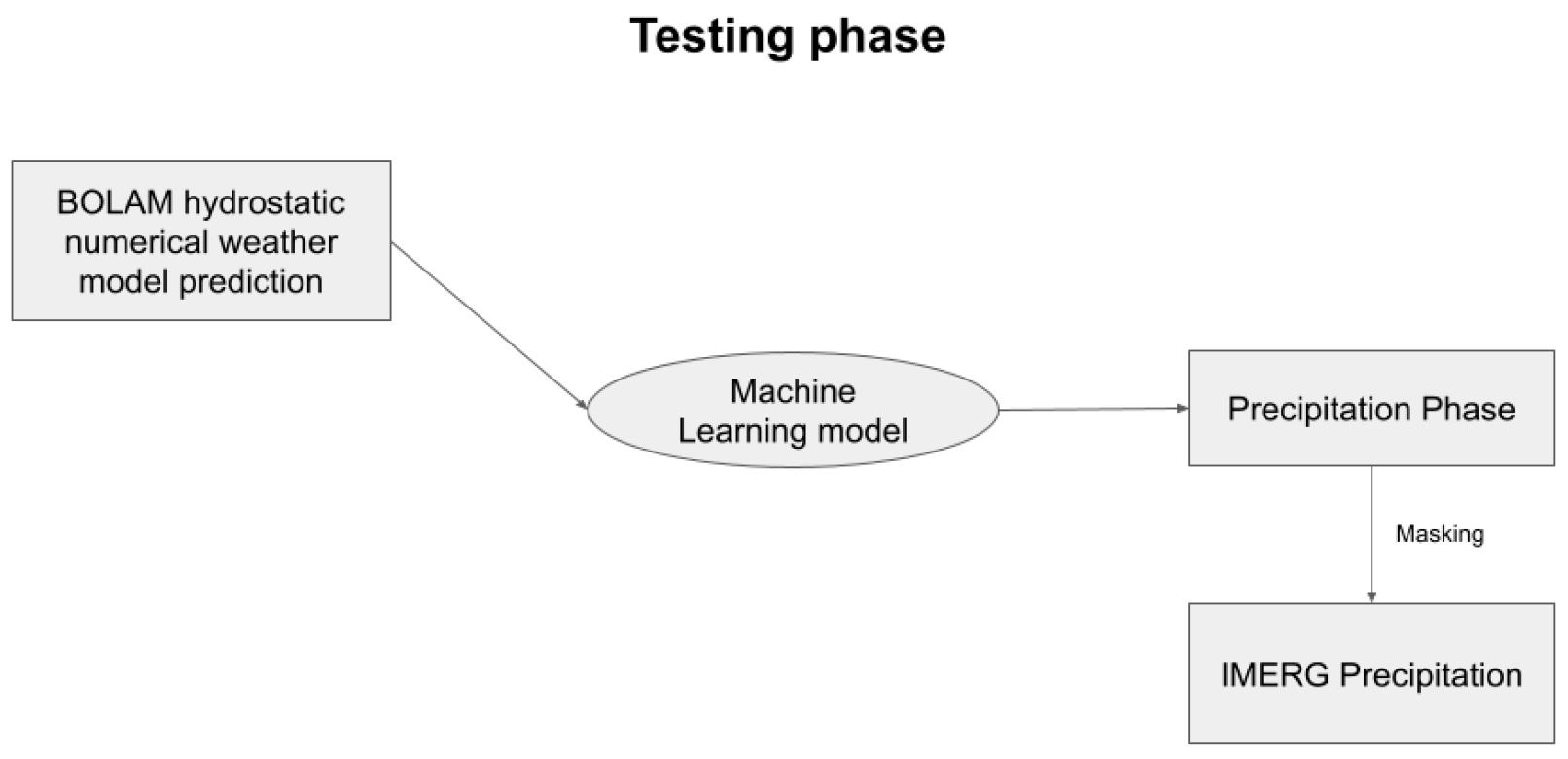
2.4. Training and Testing Process

Data are divided into training and testing datasets using an 80:20 ratio. This is accomplished using a fivefold cross-validation technique, ensuring that data for each station location are exclusively present in only one of the two datasets during each iteration. The models described above are trained using the training data (Figure 2), comprising 80% of the whole. Finally, the trained models are tested on the corresponding testing dataset (Figure 3) and their performance is calculated for each fold. The average performance of the models across all iterations is then calculated.

For the gradient boosting model, the XGBClassifier from the XGBoost library is used. Maximum depth is set to 10, learning rate is set to 1.5 × 10⁻¹, and the number of estimators is 100.

For the feedforward neural network, PyTorch machine learning framework was utilized. The architecture of the model contains linear layers with 512 neurons, as well as ReLU and sigmoid activation functions. The number of hidden layers is set to 11 with Rectified Linear Unit (ReLU) activation functions before and after each layer. A sigmoid activation function is applied to the output layer, thus transforming the output into probabilities. To train the network, the learning rate is set to 1 × 10⁻⁵ and 10 epochs are used.

2.5. Evaluation and Metrics

The metrics used to evaluate the results of the models are precision, recall (also called probability of detection) and Heidke Skill Score.

Precision (Equation (1)) is a statistical metric that measures the proportion of the true positive (TP) results among all the positive results predicted by the model, showing how many of the positive results the model predicted are actually correct and not false positive (FP). A value of 0 indicates complete disagreement between forecast and observations, while a value of 1 indicates a perfect forecast.

Precision = TP/(TP + FP)

(1)

Recall (Equation (2)) is a statistical metric that measures the proportion of the TP results among all the actual positive cases of a dataset (TP and False Negative—FN). It represents the ability of the model to identify positive cases and is also called probability of detection. As in precision, a value of 0 indicates complete disagreement between forecast and observations, while a value of 1 indicates a perfect forecast.

Recall = TP/(TP + FN)

(2)

The Heidke Skill Score (Equation (3)) is a skill-corrected verification metric which also takes into account the number of correct random forecasts. It is derived by dividing the total number of correct forecasts minus the number of correct random forecasts by the total number of forecasts minus the number of correct random forecasts. It measures the improvement of the forecast over a chance forecast. Here, negative values indicate a forecast worse than random chance, a value of 0 means no skill level, while a value of 1 is a perfect forecast [20].

Heidke Skill Score = 2 × (TP × TN − FP × FN)/[(TP + FN) × (FN + TN) + (TP + FP) × (FP + TN)]

(3)

3. Results

Evaluation on the Testing Dataset

The three score metrics were calculated for both the gradient boosting and the feedforward neural network models on the testing dataset, with regard to their ability to predict cases with conditions favorable for snowfall. Results are shown in

Table 1. Average scores for predicting case with conditions favorable for snowfall, evaluated on the testing dataset using a 5-fold cross-validation.

Model	Precision	Recall (POD)	Heidke Skill Score
Gradient Boosting	0.87	0.76	0.80
Feedforward Neural Network	0.82	0.71	0.75

.

4. Discussion

Both machine learning models used in this study, gradient boosting and a feedforward neural network, demonstrated strong performance in identifying snowfall cases near the surface of the ground, considering a Tw of 1.1 °C as the upper threshold for solid precipitation to occur over land. Across all metrics evaluated, including the ones described in the previous sections, both models achieved very good results on the testing dataset.

5. Conclusions

During this study, an algorithm that is able to identify the precipitation phase of IMERG precipitation data was developed, leveraging a machine learning model based on gradient boosting and a deep learning model employing a feedforward neural network. A Tw of 1.1 °C was used as an upper threshold for solid precipitation to occur over land. The results of our analysis indicate that the use of machine learning models is a very promising approach for estimating the precipitation phase. Specifically, it was found that 76% of the actual snow-favorable conditions can be identified, while 87% of the predicted snow-favorable conditions proved correct.

While our study has several strengths, it is not without limitations. For example, the Tw threshold applied to distinguish between solid and liquid precipitation in in situ observational data is not the optimal indicator for the actual precipitation phase. It is planned to make use of additional in situ snowfall data from NOAAN in order to evaluate the developed models.

References

1. Skofronick-Jackson, G.; Kulie, M.; Milani, L.; Munchak, S.J.; Wood, N.B.; Levizzani, V. Satellite estimation of falling snow: A global precipitation measurement (GPM) core observatory perspective. J. Appl. Meteorol. Clim. 2019, 58, 1429–1448. [Google Scholar] [CrossRef] [PubMed]
2. Sims, E.M.; Liu, G. A Parameterization of the Probability of Snow–Rain Transition. J. Hydrometeorol. 2015, 16, 1466–1477. [Google Scholar] [CrossRef]
3. Froidurot, S.; Zin, I.; Hingray, B.; Gautheron, A. Sensitivity of Precipitation Phase over the Swiss Alps to Different Meteorological Variables. J. Hydrometeorol. 2014, 15, 685–696. [Google Scholar] [CrossRef]
4. Liao, L.; Meneghini, R.; Iguchi, T.; Detwiler, A. Use of Dual-Wavelength Radar for Snow Parameter Estimates. J. Atmos. Ocean. Technol. 2005, 22, 1494–1506. [Google Scholar] [CrossRef]
5. NASA GPM. Available online: https://gpm.nasa.gov/resources/faq/how-do-various-forms-precipitation-map-imerg-probabilityliquidprecipitation-data (accessed on 12 May 2023).
6. Behrangi, A.; Yin, X.; Rajagopal, S.; Stampoulis, D.; Ye, H. On distinguishing snowfall from rainfall using near-surface atmospheric information: Comparative analysis, uncertainties and hydrologic importance. Q. J. R. Meteorol. Soc. 2018, 144, 89–102. [Google Scholar] [CrossRef]
7. Pradhan, R.K.; Markonis, Y.; Vargas Godoy, M.R.; Villalba-Pradas, A.; Andreadis, K.M.; Nikolopoulos, E.I.; Papalexiou, S.M.; Rahim, A.; Tapiador, F.J.; Hanel, M. Review of Gpm Imerg Performance: A Global Perspective. Remote Sens. Environ. 2022, 268, 12754. [Google Scholar] [CrossRef]
8. You, Y.; Peters-Lidard, C.; Ringerud, S.; Haynes, J.M. Evaluation of Rainfall-Snowfall Separation Performance in Remote Sensing Datasets. Geophys. Res. Lett. 2021, 48, e2021GL094180. [Google Scholar] [CrossRef]
9. Rebala, G.; Ravi, A.; Churiwala, S. An Introduction to Machine Learning; Springer: Cham, Switzerland, 2019; pp. 1–17. [Google Scholar] [CrossRef]
10. Chase, R.J.; Harrison, D.R.; Burke, A.; Lackmann, G.M.; McGovern, A. A machine learning tutorial for operational meteorology. Part I: Traditional machine learning. Weather Forecast. 2022, 37, 1509–1529. [Google Scholar] [CrossRef]
11. Matsuo, T.; Sasyo, Y. Melting of snowflakes below freezing level in the atmosphere. J. Meteor. Soc. Jpn. 1981, 59, 10–25. [Google Scholar] [CrossRef]
12. Tang, G.; Long, D.; Behrangi, A.; Wang, C.; Hong, Y. Exploring Deep Neural Networks to Retrieve Rain and Snow in High Latitudes Using Multisensor and Reanalysis Data. Water Resour. Res. 2018, 54, 8253–8278. [Google Scholar] [CrossRef]
13. Huffman, G.J.; Stocker, E.F.; Bolvin, D.T.; Nelkin, E.J.; Tan, J. GPM IMERG Early Precipitation L3 Half Hourly 0.1 Degree × 0.1 Degree V06; Goddard Earth Sciences Data and Information Services Center (GES DISC): Greenbelt, MD, USA, 2019. [Google Scholar] [CrossRef]
14. Lagouvardos, K.; Kotroni, V.; Bezes, A.; Koletsis, I.; Kopania, T.; Lykoudis, S.; Mazarakis, N.; Papagiannaki, K.; Vougioukas, S. The automatic weather stations NOANN network of the National Observatory of Athens: Operation and database. Geosci. Data J. 2017, 4, 4–16. [Google Scholar] [CrossRef]
15. Lagouvardos, K.; Kotroni, V.; Koussis, A.; Feidas, H.; Buzzi, A.; Malguzzi, P. The Meteorological Model BOLAM at the National Observatory of Athens: Assessment of Two-Year Operational Use. J. Appl. Meteorol. 2003, 42, 1667–1678. [Google Scholar] [CrossRef]
16. Dafis, S.; Lolis, C.J.; Houssos, E.E.; Bartzokas, A. The atmospheric circulation characteristics favouring snowfall in an area with complex relief in Northwestern Greece. Int. J. Climatol. 2015, 36, 3561–3577. [Google Scholar] [CrossRef]
17. Chen, T.; Guestrin, C. XGBoost: A scalable tree boosting system. In Proceedings of the 22nd ACM SIGKDD International Conference on Knowledge Discovery and Data Mining, New York, NY, USA, 13–17 August 2016. [Google Scholar] [CrossRef]
18. Svozil, D.; Kvasnicka, V.; Pospichal, J. Introduction to multi-layer feed-forward neural networks. Chemom. Intell. Lab. Syst. 1997, 39, 43–62. [Google Scholar] [CrossRef]
19. Baum, E.B. On the capabilities of multilayer perceptrons. J. Complex. 1988, 4, 193–215. [Google Scholar] [CrossRef]
20. NOAA Forecast Verification Glossary. Available online: https://www.swpc.noaa.gov/sites/default/files/images/u30/Forecast%20Verification%20Glossary.pdf (accessed on 12 May 2023).
Figure 1. The NOAAN weather stations used (red dots) and the corresponding grids of BOLAM and IMERG over the Attica region.
Environsciproc 26 00103 g001
Figure 2. Schematic representation of the training phase.
Environsciproc 26 00103 g002
Figure 3. Schematic representation of the testing phase.
Environsciproc 26 00103 g003