Casimir–Lifshitz Frictional Heating in a System of Parallel Metallic Plates

Abstract

The Casimir–Lifshitz force of friction between neutral bodies in relative motion, along with the drag effect, causes their heating. This paper considers this frictional heating in a system of two metal plates within the framework of fluctuation electromagnetic theory. Analytical expressions for the friction force in the limiting cases of low (zero) temperature and low and high speeds, as well as general expressions describing the kinetics of heating, have been obtained. It is shown that the combination of low temperatures (T < 10 K) and velocities of 10–10³ m/s provides the most favorable conditions when measuring the Casimir–Lifshitz friction force from heat measurements. In particular, the friction force of two coaxial disks of gold 10 cm in diameter and 500 nm in thickness, one of which rotates at a frequency of 10–10³ rps (revolutions per second), can be measured using the heating effect of 1–2 K in less than 1 min. A possible experimental layout is discussed.

1. Introduction

Over the past two decades, much effort has been spent investigating the static [1,2] and dynamic [3,4] Casimir effect in various geometric configurations, including a system of two parallel metal (dielectric) plates separated by a narrow vacuum gap. The main objectives of these studies are the properties of a fluctuating electromagnetic field and its interaction with matter on the nanoscale. Measurement of these effects paves the way to the core of nonequilibrium quantum field theory [5,6,7,8].

In addition to the attractive (in most cases) Casimir forces between electrically neutral bodies at rest, a dissipative tangential force arises when one or both bodies move relative to each other. The sources of these forces are dissipative effects within the plates (Joule losses). In this case, the corresponding fluctuation electromagnetic forces are called “van der Waals” [9], “Casimir” [10], or “quantum” [11] forces of friction. As it looks, it is convenient to use the general name “Casimir-Lifshitz” (CL) friction force, which incorporates all the features of these dissipative forces regarding their distance, temperature, and material properties.

It is worth noting that, despite of many intense efforts, no convincing experimental measurements of CL friction forces have been carried out to date. This is due not only to the small magnitude of these forces relative to the “ordinary” Casimir forces (forces of attraction) but also to the imperfections of the measurement layout. In particular, the effective interaction area and relative velocity are significantly limited in the “pendulum” measurement scheme used in Ref. [12]. Other experimental scenarios [9,13,14,15,16,17] seem to be more exotic. Recently, in Refs. [15,16,17], to measure traces of quantum friction, the authors suggested a scenario in which the nitrogen vacancy center in diamond acquires the geometric phase during rotation at a frequency of 10³–10⁴ rps (revolutions per second) near the Si- or Au-coated surface. Nitrogen vacancy centers have been proposed for use as the main components of quantum computer processors [18].

Nearly all experiments to measure Casimir–Lifshitz forces (both conservative and dissipative) have been performed with well-conducting materials (metals like gold) under near-normal temperature conditions. Regarding Casimir–Lifshitz friction forces, it has usually been assumed that they decrease with decreasing temperature as the resistivity of metals and ohmic losses decrease. Therefore, at first glance, the friction force also does. The conclusion that for metals, the temperature behavior of CL friction is not that simple was first made in Ref. [19] and later discussed in [20,21]. It has been shown that at temperatures T << θ_D (θ_D is the Debye temperature), the force of friction can increase by several orders of magnitude compared with normal conditions. However, several issues have not been elucidated, in particular, the relation between friction and heating effects at thermal nonequilibrium, the relation between quantum friction and friction at close to zero temperature, and the kinetics of radiation heating, etc. In particular, the interplay between nonequilibrium dynamics, the quantum and thermal properties of the radiation, and the confinement of light at the vacuum-surface interface may lead to several intriguing features caused by nonequilibrium thermodynamics of quantum friction [22,23,24,25]. Some other effects were considered in Refs. [26,27,28,29,30].

The main objective of this paper, in addition to studying CL friction and heating in a system of parallel metallic plates of nonmagnetic metals like gold, is to substantiate the possibility of determining the friction force from thermal measurements. In the calculations, the general results of fluctuation electrodynamics [31,32] are used, without a linear expansion in velocity in the basic expressions. It is shown that identical metal plates with different initial temperatures, moving with a constant nonrelativistic velocity, $V$, relative to each other, rapidly reach a state of quasithermal equilibrium and continue to heat up further. The heating rate is then determined by the power of the friction force.

The outline of this paper is as follows. In Section 2, the general relations between radiative heating and friction force for parallel plates in relative nonrelativistic motion are given. In Section 2.2, Section 2.3, Section 2.4, Section 2.5 I consider the simplest case of identical plates of Drude metals having the same material parameters and temperature, $T$. Analytical expressions are obtained for the friction force of metal plates in the limiting cases of low (zero) temperature and low and high speeds, as well as general expressions describing the kinetics of heating. In Section 3, the results of the numerical calculations (heating rates of plate 1 and friction parameter, $\eta =F_x/V,$ with F_x the x-component of the friction force) are given for different thermal configurations and velocities. The analytical results of Section 2 are compared with the results of numerical integration according to the general formulas. Section 4 is devoted to a brief discussion of a possible layout of an experiment for determining the CL friction force by measuring the heating rates of gold plates. Concluding remarks are given in Section 5. Appendix A, Appendix B and Appendix C contain the details of the analytical calculations. All formulas are written in the Gaussian units, $\hslash \mathrm{a}\mathrm{n}\mathrm{d} c$ are the reduced Planck constant and the speed of light in vacuum, respectively, $T$ denotes the absolute temperature and is given in units of energy.

2. General Results

2.1. Radiative Heating and Friction Force for Parallel Plates in Relative Motion

Here, we use the standard formulation of the problem, in which the plates are assumed to be made of homogeneous and isotropic materials with permittivities, ${\epsilon }_1$, ${\epsilon }_2$, and permeabilities, ${\mu }_1, {\mu }_2$, depending on the frequency, $\omega ,$ and local temperatures, $T_1$ and $T_2$ (Figure 1).

In line with Refs. [31,32], the power, $F_{x}V$, of the friction force x-component, $F_x,$ per unit surface area applied to plate 2 in the laboratory coordinate system associated with plate 1 is calculated using

$$F_{x}V=P_1+P_2/\gamma .$$

(1)

Here, $P_1$ and $P_2$ are the heat fluxes of the plates from a unit surface area per unit time, and $\gamma ={\left(1-V^2/c^2\right)}^{-1/2}$. For all quantities, indices 1 and 2 here and in what follows correspond to the numbering in Figure 1. Moreover, $P_1$ and $P_2$ are calculated in the rest frames of the plates. General relativistic expressions for $P_1$ and $P_2$ were obtained in Ref. [31]. In the nonrelativistic case, $V/c\ll 1$, but taking retardation into account, a more compact form of $P_1$ and $P_2$ reads [32]:

$$P_1=\frac{\hslash }{4{\pi }^3}\underset{0}{\overset{\infty }{\int }}d\omega \omega \int d^{2}k\frac{{\left|q\right|}^2}{{\left|Q_{\mu }\right|}^2}\mathrm{I}\mathrm{m}\left(\frac{q_1}{{\mu }_1}\right)\mathrm{I}\mathrm{m}\left(\frac{{\tilde{q}}_2}{{\mu }_2}\right)\left[\mathrm{c}\mathrm{o}\mathrm{t}\mathrm{h}\left(\frac{\hslash \omega }{2T_1}\right)-\mathrm{c}\mathrm{o}\mathrm{t}\mathrm{h}\left(\frac{\hslash {\omega }^{-}}{2T_2}\right)\right]+\left({\mu }_{\mathrm{1,2}}\leftrightarrow {\epsilon }_{\mathrm{1,2}}\right),$$

(2)

$$P_2=-\frac{\hslash }{4{\pi }^3}\underset{0}{\overset{\infty }{\int }}d\omega \int d^{2}k{\omega }^{-}\frac{{\left|q\right|}^2}{{\left|Q_{\mu }\right|}^2}\mathrm{I}\mathrm{m}\left(\frac{q_1}{{\mu }_1}\right)\mathrm{I}\mathrm{m}\left(\frac{{\tilde{q}}_2}{{\mu }_2}\right)\left[\mathrm{c}\mathrm{o}\mathrm{t}\mathrm{h}\left(\frac{\hslash \omega }{2T_1}\right)-\mathrm{c}\mathrm{o}\mathrm{t}\mathrm{h}\left(\frac{\hslash {\omega }^{-}}{2T_2}\right)\right]+\left({\mu }_{\mathrm{1,2}}\leftrightarrow {\epsilon }_{\mathrm{1,2}}\right),$$

(3)

$$Q_{\mu }=\left(q+q_1/{\mu }_1\left)\right(q+{\tilde{q}}_2/{\tilde{\mu }}_2)\mathrm{e}\mathrm{x}\mathrm{p}(qa\right)-\left(q-q_1/{\mu }_1\left)\right(q-{\tilde{q}}_2/{\tilde{\mu }}_2\left)\right(-qa\right), Q_{\mu }{\leftrightarrow Q}_{\epsilon }.$$

(4)

Here, ${\omega }^{-}=\omega -k_{x}V$, $q=\sqrt{k^2-{\omega }^2/{\mathrm{c}}^2},$ $q_{\mathrm{1,2}}=\sqrt{k^2-{\epsilon }_{\mathrm{1,2}}{\mu }_{\mathrm{1,2}}{\omega }^2/{\mathrm{c}}^2}$, and $a$ is the gap width in Figure 1. Variables with a tilde, such as ${\tilde{q}}_2,$ should be used replacing $\omega \to {\omega }^{-}$. The terms $\left({\mu }_{\mathrm{1,2}}\leftrightarrow {\epsilon }_{\mathrm{1,2}}\right)$ are defined by the same expressions with appropriate replacements. In the general case, the expressions depending on ${\epsilon }_{\mathrm{1,2}}$ and ${\mu }_{\mathrm{1,2}}$ correspond to the contributions of electromagnetic modes with P (transverse magnetic, TM) and S (transverse electric, TE) polarizations. The quantities $P_1$ and $P_2$ are directly related to the heating (cooling) rates of the plates: $d{Q}_1/dt=-P_1$ and $d{Q}_2/dt=-P_2$, where t denotes the time.

Using Equations (1)–(4), the power of the friction force $F_{x}V=P_1+P_2$ takes the form:

$$F_{x}V=\frac{\hslash }{4{\pi }^3}\underset{0}{\overset{\infty }{\int }}d\omega \int d^{2}k\left(k_{x}V\right)\frac{{\left|q\right|}^2}{{\left|Q_{\mu }\right|}^2}\mathrm{I}\mathrm{m}\left(\frac{q_1}{{\mu }_1}\right)\mathrm{I}\mathrm{m}\left(\frac{{\tilde{q}}_2}{{\mu }_2}\right)\left[\mathrm{c}\mathrm{o}\mathrm{t}\mathrm{h}\left(\frac{\hslash \omega }{2T_1}\right)-\mathrm{c}\mathrm{o}\mathrm{t}\mathrm{h}\left(\frac{\hslash {\omega }^{-}}{2T_2}\right)\right]+\left({\mu }_{\mathrm{1,2}}\leftrightarrow {\epsilon }_{\mathrm{1,2}}\right).$$

(5)

Formula (5) can be also recast into a more familiar form in terms of the Fresnel reflection coefficients [9,32].

At $T_1=T_2=T$, due to the symmetry of the system, the heating rates of identical plates are equal. One then has $F_{x}V=2P_{\mathrm{1,2}}$, and the friction force can be determined using the heating rate of any plate. For $T_1\ne T_2$, it follows that $P_1\ne P_2$, but $P_1\left(T_1,T_2\right)=P_2\left(T_2,T_1\right)$ and, correspondingly, $P_1\left(T_1,T_2\right)+P_2\left(T_1,T_2\right)=P_1\left(T_1,T_2\right)+P_1\left(T_2,T_1\right)=P_2\left(T_1,T_2\right)+P_2\left(T_2,T_1\right)$. This means that when measuring the CL friction force, it is sufficient to control the temperature of only one plate.

2.2. Metal Plates in the Drude Model

In order to treat the problem of temperature-dependent CL friction force between ordinary metals, they are described using the Drude model in terms of plasma frequency, ${\omega }_p,$ and damping parameter, $\nu \left(T\right)={\omega }_p^2\rho \left(T\right)/4\pi$, with $\rho \left(T\right)$ being the resistivity:

$$\epsilon \left(\omega \right)=1-\frac{{\omega }_p^2}{\omega \left(\omega +\mathrm{i}·\nu \left(T\right)\right)}.$$

(6)

Figure 2 plots the dependences $\rho \left(T\right)$ corresponding to the Bloch–Grüneisen (BG) model [33] and the modified Bloch–Grüneisen (MBG) model (BG scaled in Figure 2 to the data from Ref. [34]). In the former case, the residual resistance is zero or can be specified by indicating the effective temperature, below which it is constant. In the MBG model, the residual resistivity is ${\rho }_0=2.3\times {10}^{-10}\mathsf{\Omega }·\mathrm{m}$ (see Figure 2).

Hereinafter, for simplicity, the plates are assumed been made of similar nonmagnetic metal (${\mu }_1={\mu }_2=1$) with the same plasma frequency ${\omega }_p$, but different $\nu \left(T\right)$ dependence.

Since $\epsilon \left(\omega \right)\gg 1$ for good conductors and the inequality becomes stronger as $T\to 0,$ the terms with ${\epsilon }_{\mathrm{1,2}}$ in Equations (2), (3) and (5), corresponding to modes with P-polarization, are negligible compared to the terms with ${\mu }_{\mathrm{1,2}}$, corresponding to modes with S-polarization. Therefore, in what follows, the contributions of P modes are omitted.

When calculating the integrals in (2), (3), and (5), it is convenient to introduce a new frequency variable $\omega ={\nu }_m\left(T_1,T_2\right)t$, with ${\nu }_m\left(T_1,T_2\right)=\mathrm{m}\mathrm{a}\mathrm{x}({\nu }_1\left(T_1\right),{\nu }_2\left(T_2\right))$ and ${\nu }_i\left(T_i\right), i=1, 2,$ being the damping parameters of plates 1 and 2 depending on their temperatures $T_1$ and $T_2$, respectively. The absolute value $k$ of the two-dimensional wave vector (using the polar coordinates $k,\varphi$ in the plane ${(k}_x,k_y\left)\right)$ is expressed as $k=\left({\omega }_p/c\right)\sqrt{y^2+{\beta }_m^2{t}^2}$ in the evanescent sector $k>\omega /c$ ($0\le y<\infty )$ and $k=\left({\omega }_p/c\right)\sqrt{{\beta }_m^2{t}^2-y^2}$ in the radiation sector $k<\omega /c$ ($0\le y\le {\beta }_{m}t)$. Here, the parameters ${\beta }_m={\nu }_m/{\omega }_p$, ${\alpha }_i=\hslash {\nu }_i/T_i$, ${\gamma }_i={\nu }_i/{\nu }_m$, $\lambda ={\omega }_{p}a/c$, $\zeta =(V/c){{\beta }_m}^{-1}$, and $K=\frac{\mathrm{h}{\nu }_m^2{\left({\omega }_p/c\right)}^2}{2{\pi }^3}$ are introduced. With these definitions, for $k>\omega /c$, Equations (2), (3) and (5) take the form:

$$P_1=K\underset{0}{\overset{\infty }{\int }}dt\underset{0}{\overset{\infty }{\int }}dy{y^{3}f}_1\left(t,y\right),$$

(7)

$$P_2=-K\underset{0}{\overset{\infty }{\int }}dt\underset{0}{\overset{\infty }{\int }}dy{y^{3}f}_2\left(t,y\right),$$

(8)

$$F_{x}V=K\underset{0}{\overset{\infty }{\int }}dt\underset{0}{\overset{\infty }{\int }}dy{y^3\sqrt{y^2+{\beta }_m^2{t}^2}f}_3\left(t,y\right),$$

(9)

$$f_1\left(t,y\right)=t\underset{0}{\overset{\pi }{\int }}d\varphi \frac{\mathrm{I}\mathrm{m}{w}_1\mathrm{I}\mathrm{m}{w}_2}{{\left|D\right|}^2}Z\left(t,y,\varphi \right),$$

(10)

$$f_2\left(t,y\right)=\underset{0}{\overset{\pi }{\int }}d\varphi t^{-}\frac{\mathrm{I}\mathrm{m}{w}_1\mathrm{I}\mathrm{m}{w}_2}{{\left|D\right|}^2}Z\left(t,y,\varphi \right),$$

(11)

$$f_3\left(t,y\right)=\zeta \underset{0}{\overset{\pi }{\int }}d\varphi \mathrm{c}\mathrm{o}\mathrm{s}\varphi \frac{\mathrm{I}\mathrm{m}{w}_1\mathrm{I}\mathrm{m}{w}_2}{{\left|D\right|}^2}Z\left(t,y,\varphi \right),$$

(12)

$$Z\left(t,y,\varphi \right)=\mathrm{c}\mathrm{o}\mathrm{t}\mathrm{h}\left(\frac{{\alpha }_{1}t}{2}\right)-\mathrm{c}\mathrm{o}\mathrm{t}\mathrm{h}\left(\frac{{\alpha }_2{t}^{-}}{2}\right),$$

(13)

$$w_1=\sqrt{y^2+\frac{t}{t+\mathrm{i}·{\gamma }_1}} , w_2=\sqrt{y^2+\frac{t^{-}}{t^{-}+\mathrm{i}·{\gamma }_2}} , t^{-}=t-\zeta \mathrm{c}\mathrm{o}\mathrm{s}\varphi \sqrt{y^2+{\beta }_m^2{t}^2},$$

(14)

$$D=\left(y+w_1\right)\left(y+w_2\right)\exp \left(\lambda y\right)-\left(y-w_1\right)\left(y-w_2\right)\mathrm{e}\mathrm{x}\mathrm{p}(-\lambda y).$$

(15)

In the sector $k<\omega /c$, Formulas (14) and (15) should be modified by replacing $y\to \mathrm{i}y$ and substituting ${\beta }_{m}t$ for $\infty$ in Equations (7)–(9) in the integrals over $y$. The expressions for $\mathrm{I}\mathrm{m}{w}_{\mathrm{1,2}}$ can be additionally simplified. For example, it follows that

$$\mathrm{I}\mathrm{m}{w}_1=\frac{{\left(\sqrt{{\left\{{\gamma }_1^2{y}^2+\left(1+y^2\right)t^2\right\}}^2+{\gamma }_1^2{t}^2}-{\gamma }_1^2{y}^2-\left(1+y^2\right)t^2\right)}^{1/2}\mathrm{s}\mathrm{g}\mathrm{n}(-t)}{\sqrt{2\left({\gamma }_1^2+t^2\right)}}.$$

(16)

The $\mathrm{I}\mathrm{m}{w}_2$ is defined by the same expression (16), substituting ${\gamma }_2$ for ${\gamma }_1$ and $t^{-}$ for $t$. For two identical plates at quasithermal equilibrium, it follows that ${\gamma }_1={\gamma }_2=1,$ and a simpler useful expression is obtained by expanding the square root in Equation (16) and leaving the expansion terms up to the second order:

$$\mathrm{I}\mathrm{m}{w}_1\approx \frac{\left|t\right|·\mathrm{s}\mathrm{g}\mathrm{n}(-t)}{2\sqrt{\left(1+t^2\right)\left(y^2+\left(1+y^2\right)t^2\right)}}.$$

(17)

In this case, an approximate analytical calculations can be done.

2.3. Quantum Friction

In the case $T_1=T_2=0$, corresponding to the conditions of quantum friction, the main role is played by the evanescent modes $k>\omega /c$. At finite temperatures, the evanescent modes make the dominant contribution at $a<1$ µm. This range of distances is highly promising experimentally. For this reason, hereinafter, let us consider only evanescent modes, omitting the small term ${\beta }_m^2{t}^2$ in Equations (9), (14) and other formulas. Therefore, at zero temperature, substituting the identity $Z\left(t,y,\varphi \right)=\mathrm{s}\mathrm{g}\mathrm{n}\left(t\right)-\mathrm{s}\mathrm{g}\mathrm{n}\left(t-\zeta y\mathrm{c}\mathrm{o}\mathrm{s}\left(\varphi \right)\right)$ into Equation $\left(9\right)$ yields:

$$F_{x}V=2K\zeta \underset{0}{\overset{\infty }{\int }}dy{y}^4\underset{0}{\overset{\frac{\pi }{2}}{\int }}d\varphi \mathrm{c}\mathrm{o}\mathrm{s}\varphi \underset{0}{\overset{\zeta y\mathrm{c}\mathrm{o}\mathrm{s}\varphi }{\int }}dt\frac{\mathrm{I}\mathrm{m}{w}_1\mathrm{I}\mathrm{m}{w}_2}{{\left|D\right|}^2}.$$

(18)

The most straightforward asymptotics of Equation (18) can be worked out for two identical plates in the limit of low velocities, $\zeta \ll 1$. Using Equations (15) and (17), one obtains:

$$\mathrm{I}\mathrm{m}{w}_1\mathrm{I}\mathrm{m}{w}_2\to -\frac{t(\zeta y\mathrm{c}\mathrm{o}\mathrm{s}\varphi -t)}{{4y}^2}, {\left|D\right|}^2\to \frac{1}{16}{y}^{-4}\exp \left(-2\lambda y\right).$$

(19)

Inserting Equation (19) into Equation (18) yields:

$$F_{x}V=-\frac{\pi K}{2^{12}}\frac{{\zeta }^4}{{\lambda }^2}=-\frac{\hslash {{\omega }_p}^2}{2^{13}{\pi }^2}{\left(\frac{{\omega }_p}{c}\right)}^2{\left(\frac{V}{c}\right)}^2{\left(\frac{V}{a{\nu }_0}\right)}^2=-\frac{1}{2^9}\frac{\hslash }{{{\rho }_0}^2{a}^2}{\left(\frac{V}{c}\right)}^4,$$

(20)

where ${\rho }_0$ is the residual resistivity corresponding to the zero-temperature damping factor ${\nu }_0=\nu \left(0\right).$ The limit of high velocities, $\zeta \gg 1$ is more laborious. A reasonable representation of the double integral in Equation (9) can be worked out using an approximate expression for $\mathrm{I}\mathrm{m}{w}_1\mathrm{I}\mathrm{m}{w}_2$, based on Equation (17):

$$\mathrm{I}\mathrm{m}{w}_1\mathrm{I}\mathrm{m}{w}_2=\frac{\left|t\left(b-t\right)\right|\mathrm{s}\mathrm{g}\mathrm{n}\left(t\right)\mathrm{s}\mathrm{g}\mathrm{n}(b-t)}{4{\left[\left(1+t^2\right)\left(1+{(t-b)}^2\right)\left(y^2+t^2(1+y^2\right)\left)\left(y^2+{(t-b)}^2(1+y^2\right)\right)\right]}^{1/2}}.$$

(21)

where $b=\zeta y\mathrm{c}\mathrm{o}\mathrm{s}\varphi$. The product $\mathrm{I}\mathrm{m}{w}_1\mathrm{I}\mathrm{m}{w}_2$, as a function of $t$ in the range $0\le t\le b,$ reaches its maximum close to the point $t=b/2$, with zeroing at the end points $t=0, t=b$ of the integration domain of the inner integral in Equation (9). At the same time, the dependence on $t$ in ${\left|D\right|}^2$ is much weaker. By virtue of this, $t=b/2$ was inserted into the denominator of Equation (21) and into ${\left|D\right|}^2$ (in the latter case, $\mathrm{c}\mathrm{o}\mathrm{s}\varphi \approx 1 \mathrm{i}\mathrm{s}\mathrm{a}\mathrm{l}\mathrm{s}\mathrm{o}\mathrm{u}\mathrm{s}\mathrm{e}\mathrm{d})$. Expression (21) then takes the form

$$\mathrm{I}\mathrm{m}{w}_1\mathrm{I}\mathrm{m}{w}_2\approx -\frac{t\left(b-t\right)}{4\left[\left(1+b^2/4\right)\left(y^2+b^2(1+y^2\right)/4)\right]}.$$

(22)

With these transformations, it follows that (see Appendix A):

$$F_{x}V=-\frac{K\zeta }{2}\underset{0}{\overset{\infty }{\int }}dy\frac{y^4}{{\left|D\right|}^2}\underset{0}{\overset{\pi /2}{\int }}d\varphi \frac{\mathrm{c}\mathrm{o}\mathrm{s}\varphi }{\psi \left(y,\varphi \right)}\underset{0}{\overset{\zeta y\mathrm{c}\mathrm{o}\mathrm{s}\varphi }{\int }}dtt\left(\zeta y\mathrm{c}\mathrm{o}\mathrm{s}\varphi -t\right),$$

(23)

where ${\left|D\right|}^2$ and $\psi \left(y,\varphi \right)$ are calculated using Equations (A2) and (A3). The integrals over $t$ and $\varphi$ are calculated explicitly, and finally, we obtain (see Equations (A4) and (A6)):

$$F_{x}V=-\frac{\hslash {{\nu }_0}^2}{3{\pi }^2}{\left(\frac{{\omega }_p}{c}\right)}^2\underset{0}{\overset{\infty }{\int }}dy\frac{y^5\exp \left(-2\lambda y\right)}{{\left(y+\sqrt{1+y^2}\right)}^4}\left(\frac{1}{y^2\left(1+y^2\right)}-\frac{2}{y^2\sqrt{y^2{\zeta }^2+4}}+\frac{2}{(1+y^2)\sqrt{(1+y^2){\zeta }^2+4}}\right).$$

(24)

As follows from Equation (24), in this approximation, the power of the quantum friction force does not depend on the velocity. However, it is worth noting that the condition $\zeta \gg 1$ implies ${\rho }_0{\omega }_p\ll 4\pi V/c$, and along with $V/c\ll 1$, it can only be satisfied if ${\rho }_0$ is more than three orders of magnitude smaller than the MBG value shown in Figure 2. Interestingly, for $\zeta \ll 1$, Equation (24) also agrees quite well with the numerical calculations and approximation (20) (see Section 3.2 below).

2.4. Low Temperatures, Linear in Velocity Approximation

In the quasiequilibrium thermal regime, $T_1=T_2=T$, for two identical metal plates in the linear in velocity approximation, Equations (5) and (9) can be recast into the form of [19,20]:

$$F_{x}V=-\frac{\hslash V^2}{8{\pi }^2}{\left(\frac{{\omega }_p}{c}\right)}^4{\alpha }^{-1}{Y}_1\left(\lambda ,\alpha \right),$$

(25)

$$Y_1(\lambda ,\alpha )={\alpha }^2\underset{0}{\overset{\infty }{\int }}\frac{dt}{{\mathrm{s}\mathrm{i}\mathrm{n}\mathrm{h}}^2(\alpha t/2)}\underset{0}{\overset{\infty }{\int }}dy{y}^5\frac{{\left(\mathrm{I}\mathrm{m}{w}_1\right)}^2}{{\left|D\right|}^2}.$$

(26)

In this limit, the friction parameter, $\eta =F_x/V,$ does not depend on $V$. It is the dependence $F_x\propto {\alpha }^{-1}$ in Equation (25) that leads to a large enhancement of friction at low temperatures, when $\alpha =\hslash \nu \left(T\right)/T\to 0,$ because the function $Y_1\left(\lambda ,\alpha \right)$ weakly depends on $\alpha .$ The main contribution to $Y_1\left(\lambda ,\alpha \right)$ in this case makes the values $t<1$, $y~1/2\lambda ~1$, and one can again use Equation (17) for $\mathrm{I}\mathrm{m}{w}_1$. Meantime, ${\alpha }^2{\mathrm{s}\mathrm{i}\mathrm{n}\mathrm{h}}^{-2}(\alpha t/2)\approx 4/t^2$ (this is a suitable approximation at $\alpha <0.3)$  $\mathrm{a}\mathrm{n}\mathrm{d} {\left|D\right|}^2\approx 16y^4\exp \left(2\lambda y\right).$ Making use of these simplifications in Equation (26), one arrives at (see Appendix B)

$$Y_1\left(\lambda ,\alpha \right)\approx \chi \left(\lambda \right)=\frac{\pi }{32}\left\{\frac{\pi }{4\lambda }\left[{\mathsf{H}}_1\left(2\lambda \right)-N_1\left(2\lambda \right)\right]-\frac{1}{4{\lambda }^2}\right\},$$

(27)

where ${\mathrm{H}}_1\left(x\right)$ and $N_1\left(x\right)$ are the Struve and Neumann functions [35], respectively. Using the series representations of these functions yields:

$$\chi \left(\lambda \right)=\left\{\begin{array}{cc}\frac{\pi }{64}\left(\frac{1}{\lambda }-\frac{1}{2{\lambda }^2}+\frac{1}{4{\lambda }^3}+\dots \right),& \lambda \gg 1,\\ \frac{\pi }{32}\left(\frac{1}{4}+\frac{2\lambda }{3}-2\lambda \left(\mathrm{l}\mathrm{n}\lambda +0.577\right)\right),& \lambda \ll 1.\end{array}\right.$$

(28)

A more straightforward and physically transparent low-temperature representation of Equation (25) is obtained by using the relation $\nu \left(T\right)={\omega }_p^2\rho \left(T\right)/4\pi$ between the damping factor and resistivity, yielding

$$F_{x}V=-\frac{1}{2\pi }{\left(\frac{V}{c}\right)}^2{\left(\frac{{\omega }_p}{c}\right)}^2\frac{T}{\rho \left(T\right)}\chi \left(\lambda \right).$$

(29)

Combining the relation $\alpha \ll 1$, which implies $\hslash \nu \left(T\right)\ll T$, and $\zeta \ll 1$, which implies the limit of low velocities $V/c\ll \nu \left(T\right)/{\omega }_p,$ one concludes that the Formula (29) holds at

$${\hslash \omega }_{p}V/c\ll \hslash \nu \left(T\right)\ll T.$$

(30)

As a result, the conditions of a low-temperature increase in friction and the applicability of the low-speed approximation are met at $V/c\ll T/{\omega }_p\hslash$. For gold, at $T=1 \mathrm{K}$, this implies $V/c\ll {1.5\times 10}^{-5}$.

According to Refs. [19,20], the dependence (29) is associated with a growing penetration depth of S-polarized electromagnetic modes and an increase in their density at low temperatures. A significant low-temperature increase in the friction parameter was also noted in the case of the movement of a metal particle above the metal surface [21].

2.5. Low Temperatures, High-Velocity Limit

The limit $\zeta \gg 1$ at finite but low temperatures ($\alpha \ll 1)$ can be analyzed similarly to the case of zero temperatures using the properties of the function (21). When substituting Equation (21) into Equation (9) with allowance for Equation (13), the first exponential term in Equation (13) makes the dominant contribution at $t~1\ll b=\zeta y\mathrm{c}\mathrm{o}\mathrm{s}\varphi$. Due to this, let us take an advantage of the substitution $\left|t-b\right|\to b$ in the denominator of Equation (21). For the second term in Equation (13), a new variable $t^{\prime }=t-b$ is introduced and the substitution $\left|t^{\prime }+b\right|\to b$ is made in the denominator of Equation (21), while the integral (9) is then determined using the large exponential factor ${\left(\exp \left(\alpha t^{\prime }\right)-1\right)}^{-1}$ at $t^{\prime }~1\ll b$. Then, taking into account these transformations in Equation (9), and summing both contributions, the double integral in Equation (9) finally takes the form (see Appendix C)

$$I\approx \frac{{\zeta }^2}{2}\underset{0}{\overset{\infty }{\int }}dy{y}^4{\left|D\right|}^{-2}\underset{0}{\overset{\frac{\pi }{2}}{\int }}d\varphi {\psi }_1(y,\varphi )\underset{0}{\overset{\infty }{\int }}dt\frac{t}{\left(e^{\alpha t}-1\right)}{\psi }_2(y,\varphi ),$$

(31)

where

$${\left|D\right|}^{-2}\approx {\left(y+\sqrt{1+y^2}\right)}^{-4}\exp \left(-2\lambda y\right),$$

(32)

$${\psi }_1(y,\varphi )={\mathrm{c}\mathrm{o}\mathrm{s}}^2\varphi {\left(1+{\zeta }^2{y}^2{\mathrm{c}\mathrm{o}\mathrm{s}}^2\varphi \right)}^{-1/2}{\left(1+{\zeta }^2({1+y^2)\mathrm{c}\mathrm{o}\mathrm{s}}^2\varphi \right)}^{-1/2},$$

(33)

and

$${\psi }_2\left(y,t\right)=\frac{1}{{\left[\left(1+t^2\right)\left(y^2+t^2(1+y^2\right)\right]}^{1/2}}.$$

(34)

To proceed further, we replace the function $t/\left(e^{\alpha t}-1\right)$ with $1/\alpha$ in the inner integral (31), which is again a good approximation for $\alpha <0.3$. The remaining integral yields:

$$\underset{0}{\overset{\infty }{\int }}dt\frac{t}{\left(e^{\alpha t}-1\right)}{\psi }_2\left(y,t\right)\approx \frac{1}{\alpha }\frac{\mathrm{K}\left(q\right)}{\sqrt{1+y^2}}, q={\left(1+y^2\right)}^{-1/2},$$

(35)

where $\mathrm{K}\left(q\right)$ is a complete elliptic integral [35]. Taking this into account, the $\varphi$ -integral in Equation (31) can be evaluated as the arithmetic mean between the integrals calculated with the limit functions on the left and right sides of the inequality (see Appendix C):

$${\mathrm{c}\mathrm{o}\mathrm{s}}^2\varphi {\left(1+{\zeta }^2\left(1+y^2\right){\mathrm{c}\mathrm{o}\mathrm{s}}^2\varphi \right)}^{-1}{<\psi }_1\left(y,\varphi \right)<{{\mathrm{c}\mathrm{o}\mathrm{s}}^2\varphi \left(1+{\zeta }^2{y}^2{\mathrm{c}\mathrm{o}\mathrm{s}}^2\varphi \right)}^{-1}.$$

(36)

Substituting Equation (A20) into Equations (31) and (9) finally yields:

$$F_{x}V=-\frac{T}{8{\pi }^2}V{\left(\frac{{\omega }_p}{c}\right)}^3{Y}_2\left(\lambda ,\zeta \right),$$

(37)

where $Y_2(\lambda ,\zeta )$ is calculated using:

$$Y_2\left(\lambda ,\zeta \right)=\underset{0}{\overset{\infty }{\int }}dy\frac{y^4{e}^{-2\lambda y}}{{\left(y+\sqrt{y^2+1}\right)}^4{\left(1+y^2\right)}^{\frac{1}{2}}}\mathrm{K}\left(\frac{1}{\sqrt{1+y^2}}\right)\left[\frac{\sqrt{1+{\zeta }^2{y}^2}-1}{y^2\sqrt{1+{\zeta }^2{y}^2}}+\frac{\sqrt{1+{\zeta }^2\left(1+y^2\right)}-1}{\left(1+y^2\right)\sqrt{1+{\zeta }^2\left(1+y^2\right)}}\right].$$

(38)

Similar to the case of quantum friction (24), the power of the friction force (37) does not depend on velocity.

To date, there are no other relevant calculations for the friction forces between metal plates, corresponding to low-temperature conditions. However, it is interesting to compare the results obtained here with those in the case of an atom moving above the metal surface [22,23]. Let us compare the dependences on the velocity and resistivity of metal for quantum friction ($T=0).$ Equation (20) has the same low-speed dependence, $F_x~V^3$, but the opposite dependence on resistivity (Equation (16) in Ref. [22]): $F_x~{\rho }_0^{-2}$ (yet the additional condition ${\rho }_0{\omega }_p\gg 4\pi V/c$ should be met). At high but nonrelativistic velocities (${\rho }_0{\omega }_p\ll 4\pi V/c)$, Equation (24) yields $F_x~{\rho }_0^2$ in contrast to $F_x~{\rho }_0$ (Equation (19) in Ref. [22]). The dependence on velocity in Equation (24) is more moderate, $F_x~V^{-1}$, which qualitatively agrees with that in Ref. [22]. The case $T>0,$ when the friction force is linear in velocity, is less informative, because the results of Refs. [22,23] correspond to room conditions. Yet, Formula (29) yields $F_x~1/{\rho }_0$ (assuming the condition (30)), which is different from that in Ref. [23]: $F_x~ {\rho \left(T\right)}^2$.

In general, one should not expect close qualitative similarity between the plate–plate and atom–plate configurations because in the latter case, the radiative energy exchange processes, according to Refs. [22,23], are determined by the specific thermal nonequilibrium in the system. In the case of macroscopic bodies, such as two plates, the system must reach a state of thermal quasiequilibrium; see Section 2.6 just below.

2.6. Kinetics of Heating of Plates

The heat transfer of plates is described using the equations

$$P_1\left(T_1,T_2\right)∆t={-h_1{\rho }_{1}c}_1\left(T_1\right)∆T_1 \mathrm{a}\mathrm{n}\mathrm{d} P_2\left(T_1,T_2\right)∆t={-h_2{\rho }_{2}c}_2\left(T_2\right)∆T_2.$$

(39)

With $c_i\left(T_i\right)$ being the specific heat capacities, $h_i$ and ${\rho }_i$ are the thicknesses and densities of materials, $P_1\left(T_1,T_2\right)$ and $P_2\left(T_1,T_2\right)$ are defined using Equations (2) and (3), and the temperature gains ${∆T}_i$ correspond to the interval of time $∆t$. The dependences $T_2\left(T_1\right)$ and $T_1\left(T_2\right)$ can be determined using the equation

$$\frac{{dT}_2}{d{T}_1}=\frac{P_1(T_1,T_2)c_1\left(T_1\right)h_1{\rho }_1}{P_2(T_1,T_2)c_2\left(T_2\right)h_2{\rho }_2}.$$

(40)

For identical plates, in Equation (40), one can use the replacements $P_2(T_1,T_2)\to P_1(T_2,T_1)$, $P_1(T_1,T_2)\to P_2(T_2,T_1)$. In what follows, only this case is considered.

When writing Equations (39) and (40), it is also assumed that the heat exchange due to radiative heat transfer occurs much slower than under thermal diffusion, and the plates acquire equal temperature at all points because of high thermal conductivity. Using the thermal diffusion equation along the normal to the plates, $\partial T/\partial t=a^2{\partial }^{2}T/\partial z^2$, the characteristic time of the heat diffusion necessary to reach thermal quasiequilibrium, is $\tau =h^2/a^2$ (where $a^2=\kappa /c\rho$, and $\kappa$ is the thermal conductivity). Then it follows that ${\tau =h}^{2}c\rho /\kappa$ and in the case of gold at $T=10 \mathrm{K}$ and $h_{\mathrm{1,2}}=h=500 \mathrm{\mu }\mathrm{m}$  $c=2.2$ J/(kg·K), $\kappa =3200$ W/(m·K), $\rho =19.8·{10}^3$ kg/m³ [36]) one obtains $\tau \simeq 3$  $\mathsf{\mu }\mathrm{s}$. In turn, the kinetics of heating induced by friction takes dozens of seconds or minutes (see Section 3.3 below), depending on the velocity and other parameters. Assuming that $P_i\left(T,T\right)=-0.5\eta (T,V)V^2$, from Equation (39) one obtains:

$$t=\frac{2h\rho }{V^2}\underset{T_0}{\overset{T}{\int }}\frac{c\left(T\right)}{\eta (T,V)}dT,$$

(41)

the heating time from the initial temperature $T_0$ to the final temperature $T$. In the simplest case of $\eta =\mathrm{c}\mathrm{o}\mathrm{n}\mathrm{s}\mathrm{t}$ and $c\left(T\right)=a_{1}T+a_2{T}^3$ (this is a typical low-temperature dependence for metals), it follows from Equation (41) that

$$T\left(t\right)={\left(-\beta +\sqrt{{\beta }^2+T_0^4+2\beta T_0^2+2\eta V^{2}t/{h\rho a}_2}\right)}^{1/2},$$

(42)

where $\beta =a_1/a_2$. At $T_1\ne T_2$ and relatively low velocities of plate 2, as follows from numerical calculations (see Section 3.1 below), the heating/cooling rates of metal plates differ only in sign, i.e., $P_1\left(T_1,T_2\right)=-P_2\left(T_1,T_2\right)$. This is the normal mode of heat transfer, when a hotter body cools down, and a colder one heats up. Then the left sides of Equation (39) can be equated, and the corresponding quasistationary temperature of the plates is calculated using:

$$T={\left(-\beta +\sqrt{{\beta }^2+\beta \left(T_1^2+T_2^2\right)+T_1^4+T_2^4}\right)}^{1/2},$$

(43)

where $T_1$ and $T_2$ are their initial temperatures. After establishing quasithermal equilibrium, the temperature of the plates will increase according to Equations (41) and (42).

3. Numerical Results

For an ideal metal without impurities and defects, within the BG model, the damping frequency $\nu \left(T\right)$ in Equation (6) is defined using the formula [33]:

$$\nu \left(T\right)=0.0212{\left(\mathsf{\Theta }/T\right)}^5\underset{0}{\overset{\mathsf{\Theta }/T}{\int }}dx{x}^5{\mathrm{s}\mathrm{i}\mathrm{n}\mathrm{h}}^{-2}(x/2) \left(\mathrm{e}\mathrm{V}\right).$$

(44)

Numerical calculations were performed using Equation (44) and the MBG approximation shown in Figure 2 (BG scaled). The used plasma frequency of gold is ${\omega }_p=9.03$ eV. All calculations were performed with a gap width of $a=10$ nm (Figure 1) unless another value is indicated. It should be noted that at distances of $a>10$ nm, the processes of radiative heat transfer and friction due to tunneling of electrons and phonons [37,38] seem do not occur or become insignificant [39,40,41].

3.1. Quantum Friction

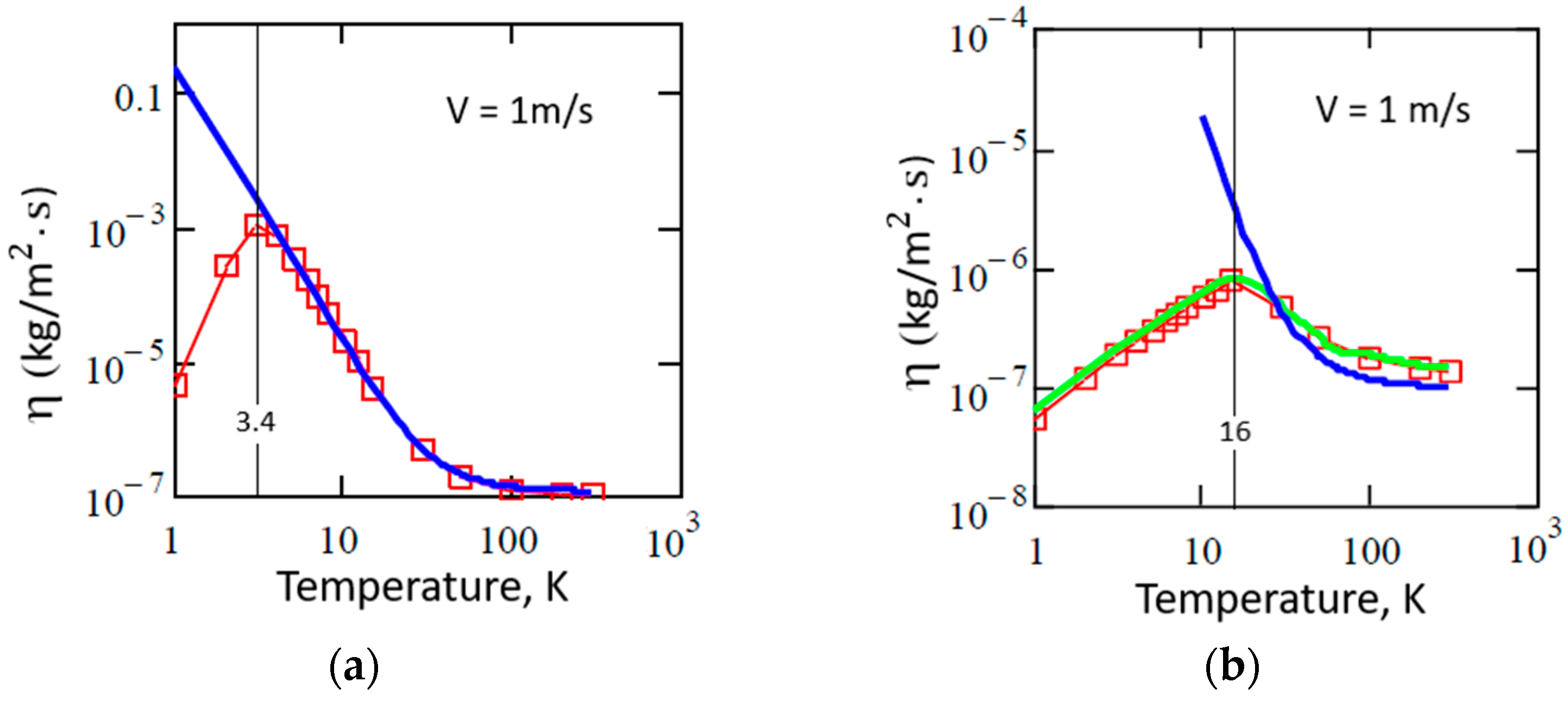
Figure 3 shows the velocity-dependent quantum friction force between the plates of gold, calculated using Formulas (20) (green line), (9) (red line) and (24) (blue line).

The curves in Figure 3a,b were calculated at residual resistances of $2.13\times {10}^{-13}$ Ω·m and $2.3\times {10}^{-10}$ Ω·m, which correspond to the BG model (44) at $T=5$ K and the MBG model at $T=0$ K. Note that in the latter case, the residual resistance coincides with that defined using Formula (44) at T = 20.9 K.

3.2. Temperature-Dependent Friction at Thermal Quasiequlibrium

Figure 4 shows the plots of the friction parameter, $\eta =F_x/V,$ depending on the temperature $T$ of the gold plates, corresponding to the BG and MBG models. The curves with symbols were calculated using Equation (9) for $V=1$ m/s. Solid curves were plotted using approximation (25) along with Equation (26) (green lines) or Equation (28) at $\lambda \gg 1$ (blue lines). In Figure 4a, both solid lines merge. The presence of maxima and their positions on the curves agree with Equations (29) and (30), respectively. These results show that the linear-in-velocity approximation is valid only to the right of the maxima of the $\eta \left(T\right)$ dependences.

Figure 5a,b demonstrates the velocity dependences of $\eta$ in the BG and MBG models. The red, blue, and green lines correspond to quasiequilibrium temperatures of 5 K, 10 K, and 77 K, respectively. The different (temperature) order of lines in Figure 5a compared to Figure 5b is explained by the high residual resistance of gold in the MBG model: the condition $\hslash \nu \left(T\right)<T$, which is necessary for the law-temperature increase in friction, is violated at $T=5$ and 10 K.

Table 1. Friction parameter $\eta$ (in kg/(m²$·$ s)) of gold plates for velocity $V=1$ m/s at thermal quasiequilibrium, Equation (9).

Temperature of Plates, K	a = 10 nm	a = 20 nm	a = 10 nm	a = 20 nm
	Model BG		Model MBG
1	4.81 × 10−6	2.77 × 10−6	5.60 × 10−8	2.80 × 10−8
2	2.63 × 10−4	1.47 × 10−4	1.22 × 10−7	5.98 × 10−8
3	1.10 × 10−3	5.73 × 10−4	1.87 × 10−7	9.13 × 10−8
5	3.44 × 10−4	1.67 × 10−4	3.08 × 10−7	1.50 × 10−7
10	2.15 × 10−5	1.04 × 10−5	5.63 × 10−7	2.73 × 10−7
15	4.30 × 10−5	2.09 × 10−6	7.77 × 10−7	3.76 × 10−7
20	1.52 × 10−6	7.35 × 10−7	7.19 × 10−7	3.33 × 10−7
50	2.04 × 10−7	9.90 × 10−8	2.56 × 10−7	1.25 × 10−7
100	1.30 × 10−7	6.30 × 10−8	1.77 × 10−7	8.63 × 10−8
200	1.14 × 10−7	5.54 × 10−8	1.42 × 10−7	6.81 × 10−8
300	1.11 × 10−7	5.41 × 10−8	1.39 × 10−7	6.81 × 10−8

shows the calculated values of the friction parameter $\eta$ of the gold plates at $V=1$ m/s, depending on the temperature, $T,$ and separation distance, a. Similar to that in Figure 4, one can note the effect of increasing friction (up to a maximum) with decreasing temperature at $T<{\theta }_D$, which is more better expressed in the BG model. The height of this maximum depends on the velocity-to-resistivity ratio. When the temperature becomes sufficiently low, condition (30) is violated, and the coefficient of friction decreases.

The dependence of $\eta$ on the separation distance a in all the cases is close to inverse proportionality ($\eta \propto a^{-1}$ ). This is clearly seen from the data in Table 1 and agrees with our previous results [19,20,32].

3.3. Friction and Heating under Different Conditions

Figure 6 and Figure 7 show the calculated heating rates of plate 1 (Figure 6a and Figure 7a) and friction parameters (Figure 6b and Figure 7b), depending on the velocity $V$ of plate 2 for various thermal configurations.

One can see that at $V<10$ m/s (Figure 6a) and $V<{10}^2$ m/s (Figure 7a), the heating rates of plates 1 and 2 are equal in absolute value, differing in sign. According to their temperatures, $T_1=4$ K and $T_2=6$ K, plate 1 heats up and plate 2 cools down, realizing the “normal” heat exchange regime. At the same time, the friction parameters weakly depend on the temperature (Figure 6b and Figure 7b). When the speed of plate 2 increases, both plates heat up faster. Then, one can see the effect of the “anomalous” heating of plate 2 for some time, when it continues to heat up despite the higher temperature. This is similar to the case of heating a hotter metal particle moving above a cold surface [21]. However, due to different absolute values of the heating rates (cf. the upper and lower lines shown with open squares (□) in Figure 6a and Figure 7a), the temperature of plate 1 “catches up” with the temperature of plate 2, and further on, both plates heat up at the same rate.

The drop in friction parameters for high velocities of plate 2 (Figure 6b and Figure 7b) is explained by the change in sign of the Doppler-shifted frequency ${\omega }^{-}=\omega -k_{x}V=\omega -kV\mathrm{c}\mathrm{o}\mathrm{s}\varphi$ in Equation (5). This occurs at $V>\nu \left(T\right)a$ because the characteristic absorption frequency is $\omega ~\nu \left(T\right)$ and the characteristic wave vector is $k~1/a$. The positions of the “kinks” on the curves $\eta \left(V\right)$ in Figure 6 and Figure 7 correlate with resistivity because $\nu \left(T\right)~\rho \left(T\right)$. Indeed, it follows from Figure 2 that ${\rho }_{\mathrm{M}\mathrm{B}\mathrm{G}}/{\rho }_{\mathrm{B}\mathrm{G}}={10}^2–{10}^3$ at T = 4–6 K. At the same time, the ratio ${\eta }_{\mathrm{M}\mathrm{B}\mathrm{G}}/{\eta }_{\mathrm{B}\mathrm{G}}$ in this case is inversely proportional to resistivities (see Equation (29) and Table 1).

In general, as follows from the calculations for all considered temperatures and velocities (Figure 5, Figure 6 and Figure 7, Table 1), the maximum friction parameter in the BG and MBG models (at $a=10$ nm) is ${10}^{-6}-{10}^{-3}$ kg/(m²·s).

Figure 8 shows the heating time of the plates versus the velocity of plate 2, calculated using numerical integration of Equation (40) from 4 K to 5 K and from 4 K to 8 K. In these calculations, the fitting parameters $a_1=0.0035 \mathrm{J}/(\mathrm{k}\mathrm{g}·{\mathrm{K}}^2)$ and $a_2=0.0023 \mathrm{J}/(\mathrm{k}\mathrm{g}·{\mathrm{K}}^4)$ of the dependence $c\left(T\right)=a_{1}T+a_2{T}^3$ were determined using the data [36] for gold at $T<20 \mathrm{K}$.

As follows from Figure 8, quite comfortable (from the experimental point of view) values of the plate heating times (1–100 s) can be obtained in the velocity range $1–{10}^3$ m/s. On the contrary, heating by 1 K at $T_0=300$ K, $a=10$ nm, and $V={10}^3$ m/s will take about 2 h. Thus, low-temperature thermal measurements have exceptional advantages over measurements under normal conditions due to a significant reduction in measurement time and the elimination of noise and other undesirable effects.

4. Experimental Proposal

Initiated by the advantage of the experimental design [15,16,17] to measure the quantum friction force, I suggested [42] using another experimental layout, as shown schematically in Figure 9. Unlike in Ref. [17], where the setup includes a disk 10 cm in diameter rotating with an angular frequency of up to ${7\times 10}^3$ rps, it is proposed to use two identical disks placed in one thermostat, one of which rotates at a controlled speed. In the peripheral region, the disks have an annular metal coating with an effective area $\pi Dw$. The non-inertiality of the reference system of disk 2 does not appear in this case because the rotation frequency is small compared to the characteristic frequencies of the fluctuation electromagnetic field. Accordingly, the original expressions (2) and (3), for heating rates remain valid.

A possible measurement scenario in this case is the quasiequilibrium thermal mode, in which the temperatures of plates increase from the initial temperature $T_0$ at the same rate. It should be noted that the experimental design must take into account possible limitations on angular velocity imposed by the tensile strength of the material used. Assuming that the main body of the plate is made of gold, a quite moderate assessment of the linear velocity of the far-distant annular parts of the plate yields $V<{\left({\sigma }_0/\rho \right)}^{0.5}$, with ${\sigma }_0=1.5{\times 10}^8$ N/m² and $\rho =1.93\times {10}^4$ kg/m³ being the tensile strength and density of gold [35]. By plugging the numerical numbers into the above condition, one obtains $V~{10}^2$ m/s, or $n ~ 300$ rps, which seems to be a well acceptable value.

5. Concluding Remarks

The Casimir–Lifshitz friction force mediated by the fluctuating electromagnetic field between metal plates moving with constant velocity relative to each other causes their heating. In a state out of thermal equilibrium, “anomalous” heating of the moving plate can be observed when it is heated for some time despite the higher temperature. However, the system rapidly reaches a state of thermal quasiequilibrium. At low temperatures $T\ll {\theta }_D$, the Casimir–Lifshitz friction and heating of metal plates increase significantly (see Equations (29) and (30)) while the heat capacity decreases. In combination with a fairly high speed of movement, this provides a fairly short heating time, which is convenient for experiments (see Equation (41)).

References

- Casimir, H.B.G. On the attraction between two perfectly conducting plates. Proc. Kon. Ned. Akad. Wetensch. B 1948, 51, 793–795. Available online: https://dwc.knaw.nl/DL/publications/PU00018547.pdf (accessed on 25 November 2023).
- Lifshitz, E.M. The theory of molecular attractive forces between solids. Sov. Phys. JETP 1956, 2, 73–83. Available online: http://jetp.ras.ru/cgi-bin/e/index/e/2/1/p73?a=list (accessed on 25 November 2023).
- Yablonovitch, E. Accelerating reference frame for electromagnetic waves in a rapidly growing plasma: Unruh-Davies-Fulling-DeWitt radiation and the nonadiabatic Casimir effect. Phys. Rev. Lett. 1956, 62, 1742–1746. [Google Scholar] [CrossRef] [PubMed]
- Dodonov, V.V.; Klimov, A.B.; Man’ko, V.I. Nonstationary Casimir effect and oscillator energy level shift. Phys. Rev. Lett. A 1989, 142, 511–513. [Google Scholar] [CrossRef]
- Schwinger, J. Casimir energy for dielectrics. Proc. Nat. Acad. Sci. USA 1989, 89, 4091–4093. [Google Scholar] [CrossRef] [PubMed]
- Dodonov, V. Fifty years of the dynamic Casimir effect. Physics 2020, 2, 67–104. [Google Scholar] [CrossRef]
- Mostepanenko, V.M. Casimir puzzle and Casimir conundrum: Discovery and search for resolution. Universe 2021, 7, 84. [Google Scholar] [CrossRef]
- Reiche, D.; Intravaia, F.; Busch, K. Wading through the void: Exploring quantum friction and vacuum fluctuations. APL Photonics 2022, 7, 030902. [Google Scholar] [CrossRef]
- Volokitin, A.I.; Persson, B.N.J. Near-field radiation heat transfer and noncontact friction. Rev. Mod. Phys. 2007, 79, 1291–1329. [Google Scholar] [CrossRef]
- Milton, K.A.; Høye, J.S.; Brevik, I. The reality of Casimir friction. Symmetry 2016, 8, 29–83. [Google Scholar] [CrossRef]
- Pendry, J.B. Shearing the vacuum–quantum friction. J. Phys. C Condens. Matter 1997, 9, 10301–10320. [Google Scholar] [CrossRef]
- Stipe, B.C.; Stowe, T.D.; Kenny, T.W.; Rugar, D. Noncontact friction and force fluctuations between closely spaced bodies. Phys. Rev. Lett. 2001, 87, 096801. [Google Scholar] [CrossRef] [PubMed]
- Volokitin, A.I. Casimir friction force between a SiO2 probe and a graphene-coated SiO2 substrate. JETP Lett. 2016, 104, 534–539. [Google Scholar] [CrossRef]
- Volokitin, A.I. Effect of an electric field in the heat transfer between metals in the extreme near field. JETP Lett. 2019, 110, 749–754. [Google Scholar] [CrossRef]
- Viotti, L.; Farias, M.B.; Villar, P.I.; Lombardo, F.C. Thermal corrections to quantum friction and decoherence: A closed time-path approach to atom-surface interaction. Phys. Rev. D 2019, 99, 105005. [Google Scholar] [CrossRef]
- Farias, M.B.; Lombardo, F.C.; Soba, A.A.; Villar, P.I.; Decca, R.S. Towards detecting traces of non-contact quantum friction in the corrections of the accumulated geometric phase. npj Quantum Inf. 2020, 6, 25. [Google Scholar] [CrossRef]
- Lombardo, F.C.; Decca, R.S.; Viotti, L.; Villar, P.I. Detectable signature of quantum friction on a sliding particle in vacuum. Adv. Quant. Technol. 2021, 4, 2000155. [Google Scholar] [CrossRef]
- Gurudev Dutt, M.V.; Childress, L.; Jiang, L.; Togan, E.; Maze, J.; Jelezko, F.; Zibrov, A.S.; Hemmer, P.R.; Lukin, D. Quantum register based on individual electronic and nuclear spin qubits in diamond. Science 2007, 316, 1312. [Google Scholar] [CrossRef]
- Dedkov, G.V. Low-temperature increase in the van der Waals friction force with the relative motion of metal plates. JETP Lett. 2021, 114, 779–784. [Google Scholar] [CrossRef]
- Dedkov, G.V. Puzzling low-temperature behavior of the van der Waals friction force between metallic plates in relative motion. Universe 2021, 7, 427. [Google Scholar] [CrossRef]
- Dedkov, G.V. Nonequilibrium Casimir-Lifshitz friction force and anomalous radiation heating of a small particle. Appl. Phys. Lett. 2022, 121, 231603. [Google Scholar] [CrossRef]
- Reiche, D.; Intravaia, F.; Hsiang, J.-T.; Busch, K.; Hu, B.-L. Nonequilibrium thermodynamics of quantum friction. Phys. Rev. 2020, 102, 050203. [Google Scholar] [CrossRef]
- Oelschläger, M.; Reiche, D.; Egerland, C.H.; Busch, K.; Intravaia, F. Electromagnetic viscosity in complex structured environments: From black-body to quantum friction. Phys. Rev. A 2022, 106, 052205. [Google Scholar] [CrossRef]
- Brevik, I.; Shapiro, B.; Silveirinha, M. Fluctuational electrodynamics in and out of equilibrium. Int. J. Mod. Phys. A 2022, 37, 2241012. [Google Scholar] [CrossRef]
- Intravaia, F. How modes shape Casimir physics. Int. J. Mod. Phys. A 2022, 37, 2241014. [Google Scholar] [CrossRef]
- Jentschura, U.D.; Lach, G.; De Kiviet, M.; Pachucki, K. One-loop dominance in the imaginary part of the polarizability: Application to blackbody and noncontact van der Waals friction. Phys. Rev. Lett. 2015, 114, 043001. [Google Scholar] [CrossRef]
- Klatt, J.; Bennett, R.; Buhmann, S.Y. Spectroscopic signatures of quantum friction. Phys. Rev. A 2016, 94, 063803. [Google Scholar] [CrossRef]
- Guo, X.; Milton, K.A.; Kennedy, G.; McNulty, W.P.; Pourtolami, N.; Li, Y. Energetics of quantum friction: Field fluctuations. Phys. Rev. D 2021, 104, 116006. [Google Scholar] [CrossRef]
- Guo, X.; Milton, K.A.; Kennedy, G.; McNulty, W.P.; Pourtolami, N.; Li, Y. Energetics of quantum friction. II: Dipole fluctuations and field fluctuations. Phys. Rev. D 2022, 106, 016008. [Google Scholar] [CrossRef]
- Milton, K.A.; Guo, X.; Kennedy, G.; Pourtolami, N.; DelCol, D.M. Vacuum torque, propulsive forces, and anomalous tangential forces: Effects of nonreciprocal media out of thermal equilibrium. arXiv 2023, arXiv:2306.02197. [Google Scholar] [CrossRef]
- Polevoi, V.G. Tangential molecular forces caused between moving bodies by a fluctuating electromagnetic field. Sov. Phys. JETP 1990, 71, 1119–1124. Available online: http://jetp.ras.ru/cgi-bin/e/index/e/71/6/p1119?a=list (accessed on 25 November 2023).
- Dedkov, G.V.; Kyasov, A.A. Friction and radiative heat exchange in a system of two parallel plate moving sideways: Levin-Polevoi-Rytov theory revisited. Chin. Phys. 2018, 56, 3002. [Google Scholar] [CrossRef]
- Condon, E.U.; Odishaw, H. (Eds.) Handbook of Physics; McGraw-Hill Book Company, Inc.: New York, NY, USA, 1967. [Google Scholar]
- Baptiste, J. Resistivity of gold. In The Physics Factbook; Elert, G., Ed.; 2004; Available online: https://hypertextbook.com/facts/2004/JennelleBaptiste.shtml (accessed on 25 November 2023).
- Gradshteyn, I.S.; Ryzhik, I.M. Table of Integrals, Series and Products; Academic Press/Elsevier Inc.: Waltham, MA, USA, 2014. [Google Scholar] [CrossRef]
- Grigoriev, I.S.; Meilikhov, E.Z. (Eds.) Handbook of Physical Quantities; CRC Press/Taylor & Francis Group: Boca Raton, FL, USA, 1996; Available online: https://archive.org/details/handbookofphysic0000unse_b1e4 (accessed on 25 November 2023).
- Biehs, S.-A.; Kittel, A.; Ben-Abdallah, P. Fundamental limitations of the mode temperature concept in strongly coupled system. Z. Naturforsch. A 2020, 75, 803–807. [Google Scholar] [CrossRef]
- Viloria, M.G.; Guo, Y.; Merabia, S.; Ben-Abdallah, P.; Messina, R. Role of Nottingham effect in the heat transfer in extreme near field regime. Phys. Rev. 2023, 107, 125414. [Google Scholar] [CrossRef]
- Pendry, J.B.; Sasihithlu, K.; Kraster, R.V. Phonon-assisted heat transfer between vacuum-separated surfaces. Phys. Rev. B 2016, 94, 075414. [Google Scholar] [CrossRef]
- Sasihithlu, K.; Pendry, J.B. Van der Waals force assisted heat transfer. Z. Naturforsch. A 2017, 72, 181–188. [Google Scholar] [CrossRef]
- Kuehn, S.; Loring, R.F.; Marohn, J.A. Dielectric fluctuations and the origins of noncontact friction. Phys. Rev. 2006, 96, 156103. [Google Scholar] [CrossRef]
- Dedkov, G.V. Casimir-Lifshitz friction force and kinetics of radiative heat transfer between metal plates in relative motion. JETP Lett. 2023, 117, 952–957. [Google Scholar] [CrossRef]
Figure 1.
Configuration of parallel plates in relative motion. See text for details.
Figure 2.
Resistivity of gold [34]. To obtain resistivity in the Gaussian units, one should use the relation . The ‘zero RR’ stands for zero residual resistance, is the Debye temperature, and denotes a linear fit. See text for more details.
Figure 3.
Quantum friction force of the plates of gold as a function of the velocity of a moving plate 2: (a) residual resistance of gold corresponds to Bloch–Grüneisen (BG) model at ; (b) residual resistance corresponds to modified BG (MBG) model at (see Figure 2). The red lines represent complete numerical integration in Equation (9), the green and blue lines are calculations using Formulas (20) and (24). The positions of the maxima and the corresponding velocities are shown, respectively, by vertical lines and the numbers indicated.
Figure 4.
Friction parameter of gold plates as a function of their quasiequilibrium temperature for (a) BG and (b) MBG models. The curves with symbols were calculated using complete numerical integration in Equation (9). Solid lines correspond to the calculations using Equation (25) with Equation (26) (green lines) and (28) (blue lines); in (a), the blue and green lines merge. The vertical numbered lines show the temperatures corresponding to the maxima of the curves.
Figure 5.
Friction parameter of gold plates as a function of the velocity of plate 2 for the (a) BG and (b) MBG models. The solid lines represent the calculations using Equation (9), dashed lines—Equations (37) and (38). The red, blue, and green lines correspond to quasistationary temperatures of 5 K, 10 K, and 77 K, respectively, for both plates. The different temperature order of the curves in (b) is explained by a different sequence of parameters : The plateau in the curves corresponds to the linear velocity dependence of the friction force.
Figure 6.
Heating rate of plate 1 (a) and friction parameter (b) as a function of velocity V of plate 2 in the BG model. The temperature configuration for the plates are indicated on the curves as follows: e.g., 6/4 denotes Thermal configurations and have the same friction parameters, configurations and correspond to a quasiequilibrium thermal mode. The data shown by open triangles (∆ (a)) and by open diamonds (◊ (b)) are multiplied by 3 (cf. [42], where all numerical data to be reduced by times).
Figure 7.
Same as in Figure 6 but in the MBG model. No additional numerical factors for the data are used.
Figure 8.
Heating time of gold plates as a function of the velocity of plate 2 at h = 500 μm according to BG (a) and MBG (b) models. Two upper lines correspond to heating from 4 K to 8 K at a = 20 nm (crimpson) and a = 10 nm (blue), and two lower lines correspond to heating from 4 K to 5 K at a = 20 nm (green) and a = 10 nm (red).
Figure 9.
A possible setup for measuring Casimir–Lifshitz friction force (side view). The thermal protection layer is shown in blue, the metal coating is shown in brown. When the upper disk rotates, the circular sections of disks locating at a distance a move at a linear velocity of relative to each other. At rotation frequencies n = 1–104 rps (revolutions per second) and disk diameter m, the velocity range to be 0.3–3000 m/s.