Opinion Dynamics Systems via Biswas–Chatterjee–Sen Model on Solomon Networks
by
 ,
,
Edmundo Alves Filho
1, 
Francisco Welington Lima
1,*,
Tayroni Francisco Alencar Alves
1,
Gladstone de Alencar Alves
2 and
Joao Antonio Plascak
3,4,5 1
Dietrich Stauffer Computational Physics Laboratory, Departamento de Física, Universidade Federal do Piauí, Teresina 64049-550, PI, Brazil
2
Departamento de Física, Universidade Estadual do Piauí, Teresina 64002-150, PI, Brazil
3
Departamento de Física, Centro de Ciências Exatas e da Natureza (CCEN), Universidade Federal da Paraíba, Cidade Universitária, João Pessoa 58051-970, PB, Brazil
4
Departamento de Física, Universidade Federal de Minas Gerais, C. P. 702, Belo Horizonte 30123-970, MG, Brazil
5
Department of Physics and Astronomy, University of Georgia, Athens, GA 30602, USA
*
Author to whom correspondence should be addressed.
Physics 2023, 5(3), 873-882; https://doi.org/10.3390/physics5030056
Submission received: 12 June 2023
/
Revised: 25 July 2023
/
Accepted: 3 August 2023
/
Published: 17 August 2023
(This article belongs to the Special Issue In Honor of Professor Serge Galam for His 70th Birthday and Forty Years of Sociophysics)
Abstract
:The critical properties of a discrete version of opinion dynamics systems, based on the Biswas–Chatterjee–Sen model defined on Solomon networks with both nearest and random neighbors, are investigated through extensive computer simulations. By employing Monte Carlo algorithms on SNs of different sizes, the magnetic-like variables of the model are computed as a function of the noise parameter. Using the finite-size scaling hypothesis, it is observed that the model undergoes a second-order phase transition. The critical transition noise and the respective ratios of the usual critical exponents are computed in the limit of infinite-size networks. The results strongly indicate that the discrete Biswas–Chatterjee–Sen model is in a different universality class from the other lattices and networks, but in the same universality class as the Ising and majority-vote models on the same Solomon networks.
1. Introduction
Although a great deal of attention has been given to sociophysics in the last forty years, it is over the past two decades that the interest in this area has been indeed enhanced, mainly due to the dynamics properties that are present in social systems or networks (see, e.g., Refs. [1,2,3,4,5,6,7,8,9]). The early models in this new scenario have been proposed by Stauffer [6] and Galam [9] using local majority rule arguments, which are also called dynamics of opinions.
There are also other models that are useful for simulating the behavior of people in a community where each person can either be influenced by the neighbors or be a means to influence these neighbors. Just to cite a few among the great variety of dynamical systems, which are be of particular interest to the present study, let us mention the Ising model (IM), originally proposed to treat the thermal properties of magnetic systems [10,11,12], the majority-vote model (MVM) [13], and the Biswas, Chatterjee, and Sen (BChS) model [5].
The IM, MVM, and BChS model have been treated by using Monte Carlo simulations on different lattices and networks. It has been noticed that the existence of a transition–whether of first or second order–and, in the latter case, the corresponding critical exponents, strongly depend on the type of the network. Magnetic models of the Ising kind have been reviewed in Ref. [14] and, more recently, the universality class of the BChS model, in comparison with the MVM, has been treated in Ref. [15]. In Ref. [15], besides regular lattices, topologies like Apollonian networks, regular and directed Barabási-Albert networks, regular and directed Erdös-Rènyi random graphs, among others, have been considered. In particular, a more recent review on the BChS model [16] has more details of what has been determined so far in this dynamical system.
From the results collected in the literature, mainly regarding the dynamics of the above models, it has been noticed that: (i) one cannot say, using just basic arguments, whether a known dynamical model, on a given network, could or could not undergo a specific phase transition and (ii) in the case the system does present a second-order phase transition, what should its universality class be.
Thus, it is worth investigating what kind of dynamic behavior the discrete BChS model presents when defined on Solomon networks (SNs). In addition, since the BChS model on SNs, to our best knowledge, has not been treated so far in the literature, it is also beneficial to compare its new behavior with the previous results obtained using different networks (and also to compare it with the IM and MVM). Actually, one can further implement Table 3 of Ref. [15]. It should be stressed that the novelty of the SNs over other networks is that the SNs have a more realistic approach to the behavior of a community of people as soon as SNs take into account the influence of different types of neighbors one faces, for example, at home and at work. This is indeed a new ingredient that has not been included in the lattices, networks, and random graphs studied so far.
Thus, in the present study, the BChS dynamical system on SNs is studied through the Monte Carlo simulations allied with the finite-size-scaling techniques. The paper is organized as follows. In Section 2, we briefly present the SNs and the BChS model in its discrete version, together with the magnetic-like variables considered here, such as the magnetization, susceptibility and the reduced fourth-order Binder cumulant. Section 2 also provides with the main ingredients of the Monte Carlo simulations employed to compute the evolution of the physical variables, which allow understanding the transition type. The results obtained are presented in Section 3. Section 4 addresses the conclusions and gives some remarks.
2. Solomon Networks, Biswas–Chatterjee–Sen Model and Monte Carlo Simulation Details
2.1. Solomon Networks
As mentioned in Section 1, the behavior of people in a community is such that each person can be influenced by the neighbors and can, at the same time, influence the neighbors. However, in reality, the neighbors at home differ from the neighbors at the workplace except, certainly, when everybody works at home. This more general situation can be modeled by using two different lattices, one representing the home lattice and the other the workplace lattice. From this general point of view, one can consider linear chains of length L and sites in one dimension (1D), and square lattices with sites in 2D (can be naturally extended to higher dimensions). If one labels by a site i () the sites in the workplace lattice, the home lattice to be labeled , to recognize is a random permutation of the order established in the workplace lattice. Thus, each person occupies two entirely different sites, i and , in the workplace lattice and home lattice, respectively. A sketch of a part of a Solomon network in two-dimensions is shown in Figure 1. From Figure 1, one can see that the neighborhood of a site on one lattice is different from the neighborhood of the corresponding permuted site on the other lattice. The one-dimensional case can be straightforwardly obtained from Figure 1.
Such a network composed of two chains or two square lattices has been suggested in Refs. [17,18]. These types of networks are called Solomon networks [19], mainly because each person is equally shared by two lattices, just as in the King Solomon’s biblical story. These SNs are also close to small-world networks [20,21]. In this way, within each lattice we have the proper type of interaction defined by the corresponding model (e.g., IM, MVM, BChS and others). As a result, the net interaction of the variables defined at site i is a sum of the corresponding interactions of the site i with its neighboring sites on the workplace lattice, added to the interactions with the neighbor sites of on the home lattice.
It is worth mentioning here that extensions can be made on the networks as well as on specific interactions on each lattice. For example, one may introduce some correlation between residence and workplace lattices, making not completely random, reflecting the situation when people select workplaces closer to their homes. More generally, instead of just representing the workplace and home, the lattices can represent any two types of groups of people, or even of more than two groups. Different topologies for the two groups could also be considered. Although all these generalizations indeed warrant further investigations, in what follows, we consider only random permutations in order not to have additional theoretical parameter.
2.2. Biswas–Chatterjee–Sen Model
The BChS model has already been treated on different regular lattices and networks [5,22,23,24]. Below, we list just the main ingredients of the model on SNs.
Each site i of SNs (having N sites) has an individual. These individuals have opinion variables defined by , at a given simulation time step t, that can take only three different values, e.g., , 0, or . The individual opinions are then updated at the following simulation time according to the BChS rules, as follows. (i) First, one initial state is constructed by randomly choosing one of the three opinion values , 0, or for each site i of the SNs. (ii) Second, a random site i is selected in order to be updated. (iii) Next, a site j (which has a bond to the previously chosen site i) is selected at random and an affinity, , is ascribed to this bond. Note that j, the corresponding site sharing the bond with site i, can be located either on the workplace lattice or home lattice. This affinity parameter, , is viewed as another discrete variable taking a positive value , with a probability q to be turned negative to . In this way, as has been shown in earlier studies [5,22,23,24], the probability q acts, in the end, as an external noise, modeling local discordances. (iv) The opinion variables are now updated as
where and are the updated opinion states of the two sites i and j, respectively, at the simulation time . Note that in these SNs, one sometimes updates sites that are not necessarily neighbors and can even be far apart. (v) Finally, when the opinion state of any site happens to be out of the interval , this site to be automatically equal to either or depending on the case of or , respectively.
2.3. Magnetic-like Variables of Interest
Averaging the opinion variables over all individuals constitutes an order parameter M, given by
where t is chosen to be large enough for the system having reached the stationary state. It has been shown that the system undergoes a phase transition, which is driven by the random configurations, in contrast to the the usual magnetic transitions driven by temperature. This means that for , where q denotes the noise probability and is its critical value, and an ordered phase is present, while for , and the system is in a disordered phase instead. indicates a second-order phase transition, in which both ordered and disordered phases become identical and highly correlated ( For more details, see [12,13,19,25]).
To fully characterize this phase transition, besides the above order parameter, one can also analyse its magnetic-like quantities, such as the order parameter fluctuation or susceptibility, , and the reduced fourth-order Binder cumulant, , which are given, respectively, by
2.4. Monte Carlo Simulation Details
The quantities (4)–(6) were computed as a function of q by using extensive Monte Carlo simulations on SNs of finite sizes ranging from , , 10,000, 30,000, 50,000, 70,000, up to 100,000 for linear chains (1D) and , , , , , up to 512 for square lattices (2D) where in the latter case . The initial Monte Carlo steps (MCSs) were discarded where, as described above in this Section, one MCS consists of randomly choosing N sites of the workplace network. The number of MCSs was found to be large enough for the systems to reach their stationary state. Next, the following MCSs were taken to compute the corresponding time averages. On the other hand, the configurational averages have been obtained by considering (for the larger lattices) to (for the smaller lattices), different initial configurations for each set of network size N and parameter q.
Close to the critical region, where , and for large networks size N, one can assume the following finite-size scaling (FSS) relations for the quantities defined in (4)–(6) (see Ref. [25]),
where , , and are the critical exponents of the order parameter, the fluctuation of the order parameter (susceptibility, )) and the correlation length, respectively. The functions, , with and , are the corresponding scaling functions, and b is a non-universal constant. The value is the corresponding critical noise for an infinite-size network. Equation (10) is the scaling behavior of the pseudo-critical noise parameter as a function of the network size N, and is estimated here as the q-value at the peak of the susceptibility.
In Section 3, the scaling laws (7)–(10) are used based on the computed values of the proper variables from the Monte Carlo simulations in order to obtain a description of the critical behavior of the model. It should be stressed here that, while for 1D networks, N is just the number of sites, for 2D networks, N is convenient to replaced with the linear size L.
3. Results and Discussion
The dependence of the reduced Binder cumulant, , on the noise parameter, q, for several finite size lattices, is shown in Figure 2a, for the (1D) case and in Figure 2b, for the (2D) case. From Figure 2, one can see that the system indeed undergoes the second-order phase transition as soon as Equation (9) does not depend on the size of the network and functions cross at the same point for different values of N apart from some finite-size effects, resulting in for (1D) and for 2D. Interestingly, the critical noise, is almost the same, within the error bars, for both types of lattices. This observation is in contrast with what one obtains by studying the IM and the MVM on the same networks. For the IM, one finds: on (1D) [26] and on 2D [27], where is the usual critical temperature (here, the number in the parentheses is the statistical error to the last digit). For the MVM, one finds: on (1D) [26] and on 2D [27], where is now the critical social temperature [27]. The above results are also shown in Table 1.
Equations (7), (8), and (10) can now be exploited to compute the ratios of the critical exponents using the critical noise, , obtained. By computing , , and the difference, , at for different values of N, while plotting the values in log scales as a function of N, a straight line is expected. What distinguishes a second-order phase transition from a first-order phase transition is the value of the exponents being different from the dimension of a lattice. The pseudo-transition noise, , is obtained from the maximum value of the susceptibility and is discussed in more details just below. The desired critical exponents ratios are thus straigtforwardly given by the slope obtained from a linear fit to the data. Typical plots of the above quantities are shown in Figure 3 as a function of the sizes N in (1D) (Figure 3a–c) and L in 2D (Figure 3d,e) on SNs. From the alignment of the data in Figure 3, one obtains an additional evidence that corroborates the transition as indeed to be in the second order case. The critical exponent ratios obtained are indicated in Figure 3 and listed in Table 2.
So far, Equations (7)–(9) have been used only to obtain the critical noise and the critical exponents. However, the equatons can be further exploited to obtain the corresponding universal scaling functions, , by analyzing the Monte Carlo data in a still wide-enough range of q. This means that when the scaled-order parameter, , the scaled susceptibility, , and the reduced Binder cumulant, , are plotted as a function of the scaled noise probability displacement, , the data collapse to a corresponding universal scaling function each. Figure 4 shows that indeed the collapse is observed for the listed scaling quantities in (1D), see Figure 4a–c, and in 2D, see Figure 4d,e, (recall that for the 2D case, N is replaced by L). The collapse shown in Figure 4 indicates the transition is indeed of a second order. Moreover, the computed critical exponents seem to be accurate, based on the present simulations.
Interestingly, the susceptibility, , presents a pronounced peak for q close to the noise transition value , as is depicted in Figure 4b for (1D) and Figure 4e for 2D. This means that one has, at , a peak with value for any of the network sizes, N or L. Thus, is assumed to be the pseudo-critical noise used in Figure 3c,f, and can also be used in Equation (8) to obtain another estimate of the critical exponents ratio, . Comparing the results in the fourth and fifth columns of Table 2, one can see that the collapse estimate of is well comparable with the critical exponents finding (fourth column in Table 2).
4. Concluding Remarks
In this paper, the discrete version of the BChS model, defined on one- and two-dimensional SNs, has been studied through extensive Monte Carlo simulations. The variables of the model, coming from the order parameter, have been computed for several values of the local consensus controlling parameter and different network sizes in both dimensions. The finite-size-scaling approach indicates that the system undergoes a second-order phase transition, as soon as the critical exponents and critical ratios certainly differ from the dimension of the network (which would imply a first-order transition instead). However, contrary to the findings in IM and MVM on the same networks, the critical noise values are found to be the same, within the statistical error, for both dimensions.
The independence of the critical point on spatial dimension is quite striking. Certainly, longer simulations would allow to positively detect the obtained equality with smaller statistical errors. Let us note that the critical noise in 2D is slightly larger than in (1D). We consider the simulations in 3D Solomon lattices to better clarify on this intriguing finding.
The BChS model in regular 1D lattices, like the IM, does not have a finite critical point. This is an expected result in classical models with short-range interactions. However, in SNs, these models can sustain an order for finite noise or finite temperatures. This transition could be associated with the fact that despite being in one dimension, due to the permutation of the sites in one of the lattices, the interactions turn out to be longer ranged, in a way that can induce a finite noise or finite temperature phase transition (recall that the 1D IM, where all spins interact with each other, has a phase transition with mean-field critical exponents). From Figure 1, one can realize that the SNs present the effective dimensionality which is higher than the corresponding embedding dimensionality.
The computed critical exponents of the BChS model on SNs are different from those obtained on regular 2D and 3D lattices [28], and are also different from those on other networks and random graphs [15]. As discussed in Section 1, this looks a general trend in these topologies, because even the existence of a phase transition is not straight enough to predict using just physical grounds. Nevertheless, the results conveyed in Table 2 strongly suggest that the BChS model, the IM and MVM fall all in the same universality class when defined on the SNs. The longer-ranged interactions may be a reason that all three models belong the same universality class. Recall that the mean-field approximation is obtained when long-range interactions are present and the exponents are independent of the model type. In addition, this may be the universality class of other similar systems in sociophysics. For completeness, we extend Table 3 of Ref. [15] by including the new universality class of the BChS model on SNs; see Table 3.
Author Contributions
Conceptualization, T.F.A.A.; Methodology and F.W.L.; Validation, E.A.F.; Formal analysis, G.d.A.A., F.W.L. and J.A.P.; Investigation, T.F.A.A.; Writing–original draft, F.W.L.; Writing–review and editing, T.F.A.A., G.d.A.A. and J.A.P.; Supervision, G.d.A.A. and J.A.P. All authors have read and agreed to the published version of the manuscript.
Funding
This research received no external funding.
Data Availability Statement
The data can be obtained from the correspondence upon a reasonable request.
Acknowledgments
Computational support provided by the system SGI Altix 1350 from the CENAPAD.UNICAMP-USP computational park, Campinas, São Paulo-Brazil, is gratefully acknowledged. The supports from Conselho Nacional de Desenvolvimento Científico e Tecnológico (CNPq), Coordenação de Aperfeiçoamento de Pessoal de Nível Superior (CAPES), A Fundação de Amparo à Pesquisa do Estado de Minas Gerais (FAPEMIG),and Fundação Cearense de Apoio ao Desenvolvimento Científico e Tecnológico (FUNCAP) are also gratefully acknowledged.
Conflicts of Interest
The authors declare no conflict of interest.
References
- Chakrabarti, B.K.; Chakraborti, A.; Chatterjee, A. (Eds.) Econophysics and Sociophysics: Trends and Perspectives; Wiley-VCH Verlag GmbH & Co. KGaA: Weinheim, Germany, 2006. [Google Scholar] [CrossRef]
- Castellano, C.; Fortunato, S.; Loreto, V. Statistical physics of social dynamics. Rev. Mod. Phys. 2009, 81, 591–646. [Google Scholar] [CrossRef]
- Helbing, D. Quantitative Sociodynamics. Stochastic Methods and Models of Social Interaction Processes; Springer: Berlin/Heidelberg, Germany, 2010. [Google Scholar] [CrossRef]
- Galam, S. Sociophysics. A Physicist’s Modeling of Psycho-Political Phenomena; Springer Science+Business Media, LLC: New York, NY, USA, 2012. [Google Scholar] [CrossRef]
- Biswas, S.; Chatterjee, A.; Sen, P. Disorder induced phase transition in kinetic models of opinion dynamics. Physica A 2012, 391, 3257–3265. [Google Scholar] [CrossRef]
- Stauffer, D. A biased review of sociophysics. J. Stat. Phys. 2013, 151, 9–20. [Google Scholar] [CrossRef]
- Sen, P.; Chakrabarti, B.K. Sociophysics: An Introduction; Oxford University Press: New York, NY, USA, 2013. [Google Scholar]
- Noorazar, H. Recent advances in opinion propagation dynamics: A 2020 survey. Eur. Phys. J. Plus 2020, 135, 521. [Google Scholar] [CrossRef]
- Galam, S.; Mod, I.J. The Trump phenomenon: An explanation from sociophysics. Int. J. Mod. Phys. B 2017, 31, 1742015. [Google Scholar] [CrossRef]
- Ising, E. Beitrag zur Theorie des Ferromagnetismus. Z. Phys. 1925, 31, 235–258. [Google Scholar] [CrossRef]
- Ising, E. Contribution to the Theory of Ferromagnetism. Available online: https://www.hs-augsburg.de/~harsch/anglica/Chronology/20thC/Ising/isi_intr.html (accessed on 29 July 2023).
- Baxter, R.J. Exactly Solved Models in Statistical Mechanics; Academic Press: London, UK, 1982. [Google Scholar]
- de Oliveira, M.J. Isotropic majority-vote model on a square lattice. J. Stat. Phys. 1992, 66, 273–281. [Google Scholar] [CrossRef]
- Lima, F.W.S.; Plascak, J.A. Magnetic models on various topologies. J. Phys. Conf. Ser. 2014, 487, 012011. [Google Scholar] [CrossRef]
- Alencar, D.S.M.; Alves, T.F.A.; Alves, G.A.; Macedo-Filho, A.; Ferreira, R.S.; Lima, F.W.S.; Plascak, J.A. Opinion dynamics systems on Barabási-Albert networks: Biswas–Chatterjee–Sen model. Entropy 2023, 25, 183. [Google Scholar] [CrossRef] [PubMed]
- Biswas, S.; Chatterjee, A.; Sen, P.; Mukherjee, S.; Chakrabarti, B.K. Social dynamics through kinetic exchange: The BChS model. Front. Phys. 2023, 11, 1196745. [Google Scholar] [CrossRef]
- Erez, T.; Hohnisch, M.; Solomon, S. Statistical economics on multi-variable layered networks. In Economics: Complex Windows; Salzano, M., Kirman, A., Eds.; Springer: Milan, Italy, 2005; pp. 201–217. [Google Scholar] [CrossRef]
- Goldenberg, J.; Shavitt, Y.; Shir, E.; Solomon, S. Distributive immunization of networks against viruses using the ‘honey-pot’ architecture. Nat. Phys. 2005, 1, 184–188. [Google Scholar] [CrossRef]
- Malarz, K. Social phase transition in Solomon network. Int. J. Mod. Phys. C 2003, 14, 561–565. [Google Scholar] [CrossRef]
- Pȩkalski, A. Ising model on a small world network. Phys. Rev. E 2001, 64, 057104. [Google Scholar] [CrossRef] [PubMed]
- Herrero, C.P. Ising model in small-world networks. Phys. Rev. E 2002, 65, 066110. [Google Scholar] [CrossRef] [PubMed]
- Lima, F.W.S.; Sumour, M.A.; Moreira, A.A.; Araújo, A.D. majority-vote and BCS model on Complex Networks. Phys. A 2021, 571, 125834. [Google Scholar] [CrossRef]
- Lima, F.W.S.; Plascak, J.A. Kinetic models of discrete opinion dynamics on directed Barabási–Albert networks. Entropy 2019, 21, 942. [Google Scholar] [CrossRef]
- Raquel, M.T.S.A.; Lima, F.W.S.; Alves, T.F.A.; Alves, G.A.; Macedo-Filho, A.; Plascak, J.A. Non-equilibrium kinetic Biswas–Chatterjee–Sen model on complex networks. Physcial A 2022, 603, 127825. [Google Scholar] [CrossRef]
- Binder, K.; Heermann, D.W. Monte Carlo Simulation in Statistical Phyics: An Introduction; Springer: Berlin/Heidelberg, Germany, 2010. [Google Scholar] [CrossRef]
- Lima, F.W.S. Equilibrium and non-equilibrium models on Solomon networks. Int. J. Mod. Phys. C 2016, 28, 1650134. [Google Scholar] [CrossRef]
- Lima, F.W.S. Equilibrium and nonequilibrium models on Solomon networks with two square lattices. Int. J. Mod. Phys. C 2017, 28, 1750099. [Google Scholar] [CrossRef]
- Mukherjee, S.; Chatterjee, A. Disorder-induced phase transition in an opinion dynamics model: Results in two and three dimensions. Phys. Rev. E 2016, 94, 062317. [Google Scholar] [CrossRef] [PubMed]
Figure 1.
Sketch of a part of Solomon network (SN) in two dimensions. The upper layer represents the workplace lattice, and the corresponding sites, labeled by i, are given by the full circles. The bottom layer represents the home lattice, with the corresponding sites labeled by the permutation and given by the full squares. The thick (straight) lines represent nearest-neighbor interactions on each layer. The curved lines specify the resulting random permutation in the home lattice of the order established in the workplace lattice.
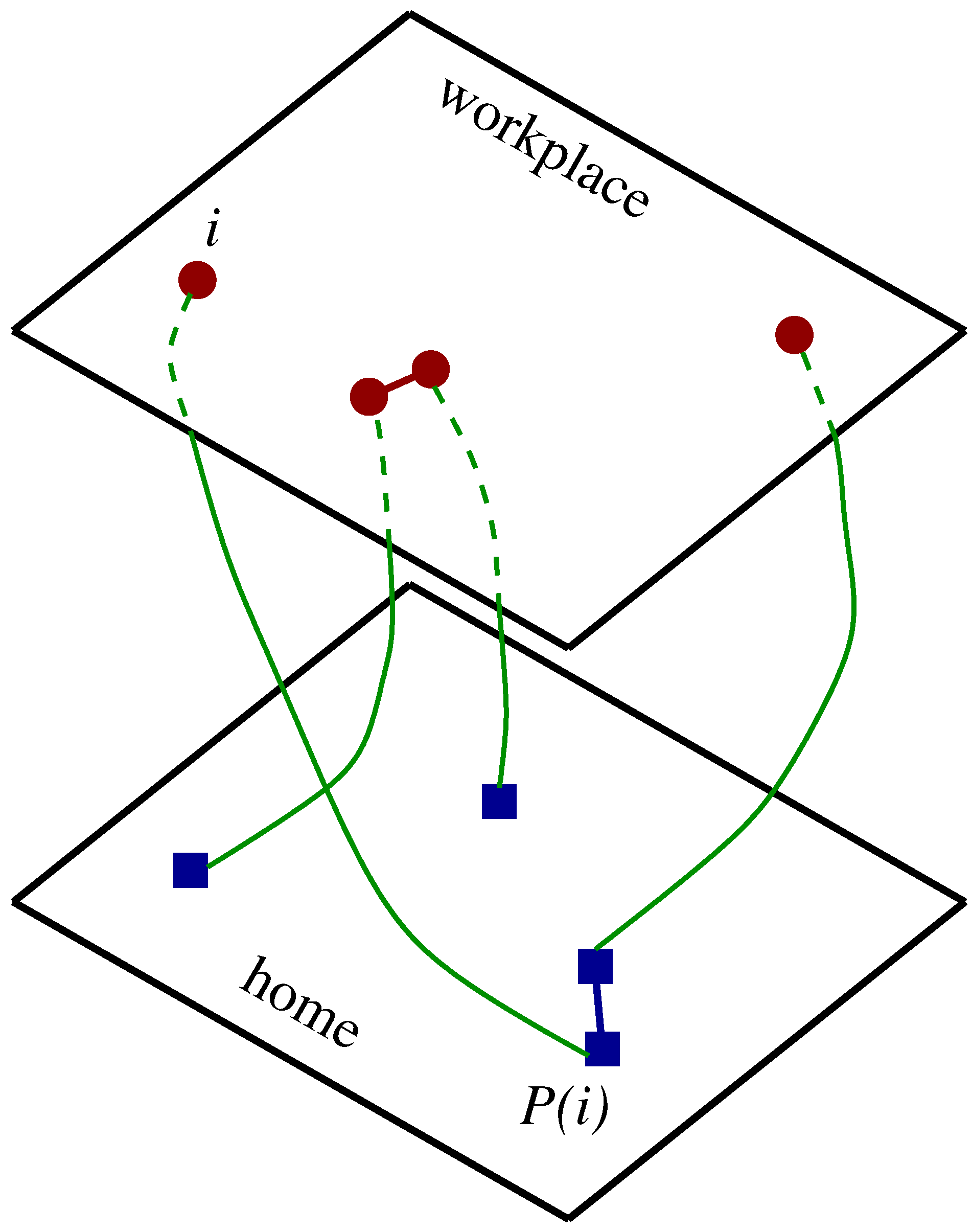
Figure 2.
Reduced Binder cumulant, , plotted as function of the noise probability, q, for one dimension (1D) (a), and 2D (b) for different values of the sizes, N (1D) and L (2D), as indicated. The crossings occur at (1D) and (2D), where the numbers in the parentheses show the statistical errors in the last digit.
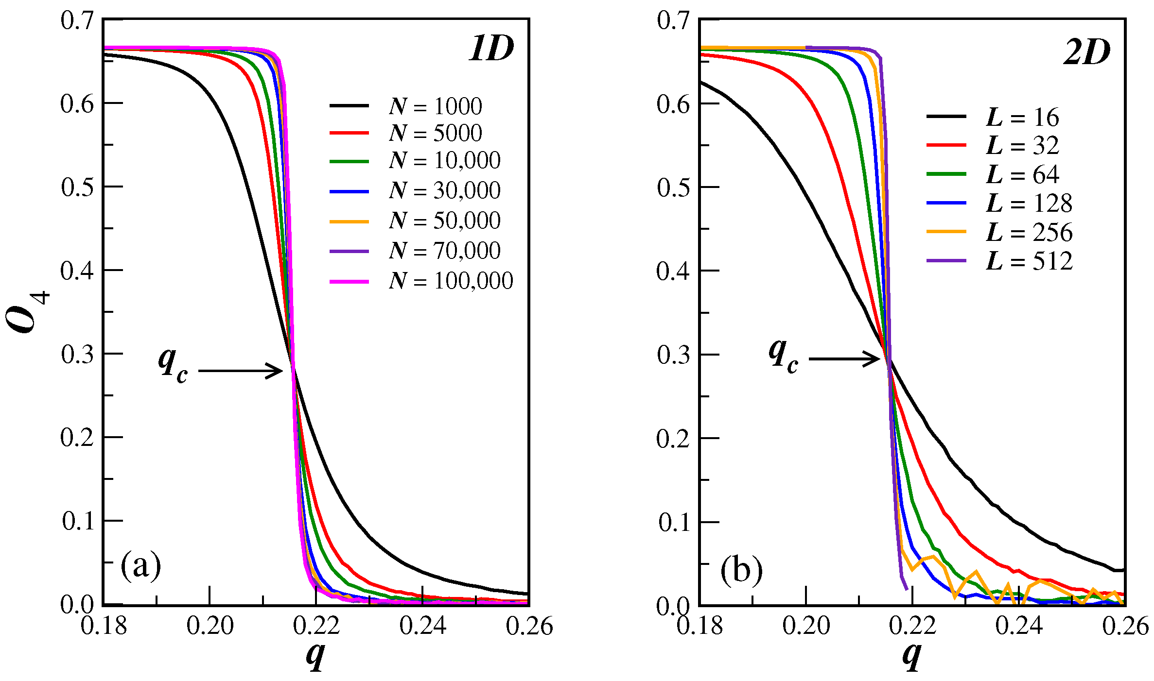
Figure 3.
Log-log plot of the order parameter, (a,d), the susceptibility, (b,e), and the magnitude of the displacement, (c,f), as a function of N (1D) and L (2D), on SNs. All quantities are computed at the extrapolated critical noise parameter, , for the corresponding dimension. The ratios of the critical exponents, , and , are shown being obtained from the slopes of the linear fits (red lines) to the data.
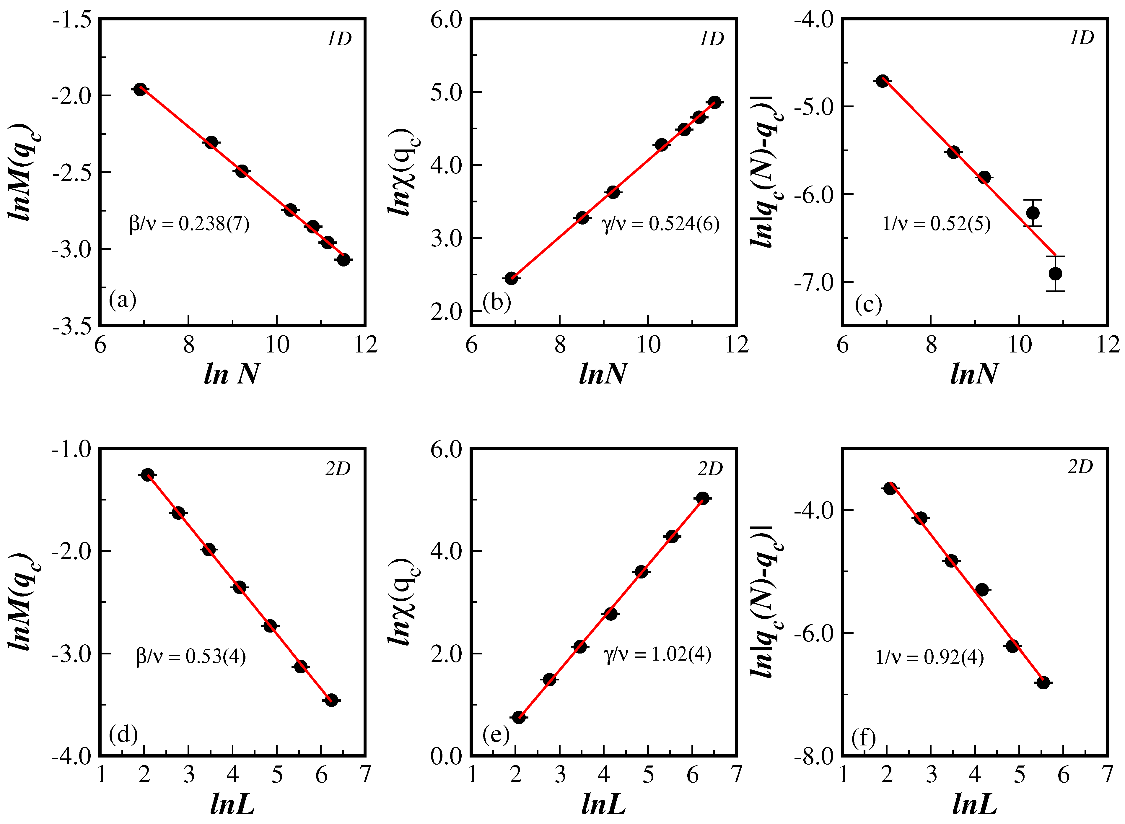
Figure 4.
Collapse of the data for the BChS model on SNs of the scaled-order parameter, (a,d), the scaled susceptibility, (b,e), and the scaled reduced Binder cumulant, (c,f) as functions of the scaled displacements, , in (1D) (a–c) and in 2D (d–f) for different values of the network sizes, N and L, as indicated.


Table 1.
Critical points (critical value, , of the noise probability, q) of the IM (thermodynamical critical temperature), MVM (critical social temperature) and (BChS) model (critical noise) in (1D) and 2D SNs. The number in the parentheses shows the statistical error in the last digit.
Table 1.
Critical points (critical value, , of the noise probability, q) of the IM (thermodynamical critical temperature), MVM (critical social temperature) and (BChS) model (critical noise) in (1D) and 2D SNs. The number in the parentheses shows the statistical error in the last digit.
| IM | MVM | BChS | |||
|---|---|---|---|---|---|
| 1D | 2D | 1D | 2D | 1D | 2D |
| 2.995(3) | 6.985(4) | 1.165(4) | 1.915(5) | 0.215(2) | 0.216(2) |
Table 2.
Critical exponents ratios, , , of the BChS model on SNs. The results obtained for the IM and the MVM on the same networks from Refs. [26,27] are included for comparison. The exponents ratio, , represents the results from the maximum of the susceptibility (see Figure 4d,e). See text for details. The number in the parentheses shows the statistical error in the last digit.
| Model | ||||
|---|---|---|---|---|
| Linear Chain (1D) | ||||
| IM [26] | ||||
| MVM [26] | ||||
| Square Lattice (2D) | ||||
| IM [27] | ||||
| MVM [27] | ||||
Table 3.
Extension of Table 3 of Ref. [15] by including the universality class of the BChS model, IM and MVM on SNs, as obtained in the present study. The “proper class” indicates that the exponents are different from any known model. z represents the connectivity of the network or random graph.
Table 3.
Extension of Table 3 of Ref. [15] by including the universality class of the BChS model, IM and MVM on SNs, as obtained in the present study. The “proper class” indicates that the exponents are different from any known model. z represents the connectivity of the network or random graph.
| Discrete Biswas–Chatterjee–Sen Model | ||
|---|---|---|
| Lattice or Network | Universality Class | Ref. |
| Fully connected | Mean field | [5] |
| Regular dimension-D | d-Dimensional IM | [28] |
| Apollonian | proper class | [22] |
| Barabási-Albert | Proper class | [15] |
| z-dependent exponents | ||
| Directed Barabási-Albert | MVM | [23] |
| z-dependent exponents | ||
| Erdös-Rènyi | Proper class | [24] |
| z-dependent exponents | ||
| Directed Erdös-Rènyi | Proper class | [24] |
| z-dependent exponents | ||
| Small world | either of | [24] |
| Erdös-Rènyi graphs | ||
| Solomon | Proper class | This paper |
| including IM and MVM | ||
| Continuum Biswas–Chatterjee–Sen model | ||
| Fully connected | Mean field | [5] |
| Regular dimension-D | d-Dimensional IM | [28] |
Disclaimer/Publisher’s Note: The statements, opinions and data contained in all publications are solely those of the individual author(s) and contributor(s) and not of MDPI and/or the editor(s). MDPI and/or the editor(s) disclaim responsibility for any injury to people or property resulting from any ideas, methods, instructions or products referred to in the content. |
© 2023 by the authors. Licensee MDPI, Basel, Switzerland. This article is an open access article distributed under the terms and conditions of the Creative Commons Attribution (CC BY) license (https://creativecommons.org/licenses/by/4.0/).
Share and Cite
MDPI and ACS Style
Filho, E.A.; Lima, F.W.; Alves, T.F.A.; Alves, G.d.A.; Plascak, J.A. Opinion Dynamics Systems via Biswas–Chatterjee–Sen Model on Solomon Networks. Physics 2023, 5, 873-882. https://doi.org/10.3390/physics5030056
AMA Style
Filho EA, Lima FW, Alves TFA, Alves GdA, Plascak JA. Opinion Dynamics Systems via Biswas–Chatterjee–Sen Model on Solomon Networks. Physics. 2023; 5(3):873-882. https://doi.org/10.3390/physics5030056
Chicago/Turabian StyleFilho, Edmundo Alves, Francisco Welington Lima, Tayroni Francisco Alencar Alves, Gladstone de Alencar Alves, and Joao Antonio Plascak. 2023. "Opinion Dynamics Systems via Biswas–Chatterjee–Sen Model on Solomon Networks" Physics 5, no. 3: 873-882. https://doi.org/10.3390/physics5030056