Article

Vector Potential, Magnetic Field, Mutual Inductance, Magnetic Force, Torque and Stiffness Calculation between Current-Carrying Arc Segments with Inclined Axes in Air

Independent Researcher, 53 Berlioz 101, Montréal, QC H3E 1N2, Canada
Physics 2021, 3(4), 1054-1087; https://doi.org/10.3390/physics3040067
Submission received: 23 September 2021 / Revised: 29 October 2021 / Accepted: 1 November 2021 / Published: 16 November 2021
(This article belongs to the Section Applied Physics)

Abstract

:
In this paper, the improved and the new analytical and semi-analytical expressions for calculating the magnetic vector potential, magnetic field, magnetic force, mutual inductance, torque, and stiffness between two inclined current-carrying arc segments in air are given. The expressions are obtained either in the analytical form over the incomplete elliptic integrals of the first and the second kind or by the single numerical integration of some elliptical integrals of the first and the second kind. The validity of the presented formulas is proved from the particular cases when the inclined circular loops are addressed. We mention that all formulas are obtained by the integral approach, except the stiffness, which is found by the derivative of the magnetic force. The novelty of this paper is the treatment of the inclined circular carting-current arc segments for which the calculations of the previously mentioned electromagnetic quantities are given.

1. Introduction

In general, a field circular coil of arbitrary geometry may be made from finite circular current-carrying arc segments of the conductor for which the magnetic field can be calculated by the sum over the partial fields generated by each segment [1,2,3,4,5,6,7,8,9,10,11,12,13,14,15,16]. This assumption significantly simplifies studying the current-carrying coils of the complex shape. In this paper, we study the inclined circular current-carrying arc segments to calculate the magnetic force, the magnetic torque, the mutual inductance, and the stiffness between them. The goal of this paper is the calculation of these electromagnetic quantities using the magnetic field of the current-carrying arc segment. The magnetic vector potential and the magnetic field of the current-carrying segment can be considered as the auxiliary functions for the simplified calculation of the previously mentioned quantities. Even though in the literature on can find many methods for calculating the magnetic vector potential and magnetic field of different current coils, we give the simplified formulas for calculating them, which will be the crucial auxiliary functions because they are given in the analytical form over the incomplete elliptic integrals of the first and second kind.
Several analytical, semi-analytical and numerical methods in the calculation of parameters of electric circuits such as the self and the mutual inductance and force interaction between their elements play a significant role in power transfer, wireless communication, sensing and actuation, and are applied in different fields of science, including electrical and electronic engineering, medicine, physics, nuclear magnetic resonance, mechatronics, and robotics [17,18,19,20,21,22,23,24,25,26,27,28,29,30,31,32,33,34,35,36,37,38]. These calculations are obtained in the form of double integrals, complete or incomplete integrals of the first, second and third kind, Bessel and Struve functions, hypergeometric series, and other special functions, so that it is difficult for the potential user to obtain fast and precise calculation. Additionally, many of these methods use filament methods which study coaxial circular coils or circular coils with parallel axes. In this paper we give a quite simple method for calculating the magnetic force and the mutual inductance between two inclined circular current-carrying arc segments in air, which can be used to calculate these parameters for inclined circular coils by using the filament method [20]. We give simple formulas for the magnetic force and the mutual inductance in the form of the single integral whose kernel functions are the incomplete integrals of the first and second kind as well as the elementary functions. Finally, we give new formulas for the calculation of the magnetic torque and the stiffness between two inclined circular current-carrying arc segments in air. They are obtained in the form of the single integral whose kernel functions are the incomplete integrals of the first and second kind. To our knowledge, these formulas appear for the first time in the literature. In all formulas, the angles of the current-carrying arcs are arbitrary. The validity of all formulas is verified with the corresponding calculations for the inclined circular loops. For the convenience of the reader, all the derived formulas were programmed using Mathematica. The Mathematica files with the implemented formulas are available from the author.

2. Basic Expressions

Let us take into consideration two current-carrying arc segments as shown in Figure 1, where the center of the larger segment (primary coil) of the radius R P is placed at the plane XOY whose center is O (0, 0, 0). The smaller circular segment (secondary coil) of the radius R S is placed in an inclined plane whose general equation is:
λ a x   +   b y   +   c z   +   d = 0 ,
where a, b and c are the components of the normal N on the inclined plane in the center of the secondary circular segment C ( x C , y C , z C ). The current-carrying arc segments are with currents I P , I S . For circular segments (see Figure 1), we define [22,23,24]:
(1) The primary circular segment of radius R P is placed in the plane XOY (Z = 0) with the center at O (0, 0, 0). An arbitrary point P ( x P , y P , z P ) of this segment has parametric coordinates,
x P = R P cos t ,   y P = R P sin t ,       z P = 0 ,       t φ 1 , φ 2 .
(2) The differential of the primary circular segment is given by
d l P = R P   sin t , cos t ,   0 d t ,           t φ 1 , φ 2 .
(3) The secondary circular segment of radius R S is placed in the inclined plane (1) with the center at C ( x c , y c , z c ). The unit vector N (the unit vector of the axis z’) at the point C, which is the center of the secondary circular segment, lying in plane λ is defined by
N =   a L , b L , c L ,       L = a 2   +   b 2   +   c 2   .
(4) The unit vector between two points C and S which are placed in plane (1) is:
u =   u x , u y , u z   =   a b L l , l L , b c L l   ,   l = a 2   +   c 2 .
(5) We define the unit vector v as the cross product of the unit vectors N and u as follows:
v = N × u =   v x , v y , z z   =   c l , 0 , a l .
(6) An arbitrary point S ( x S , y S , z S ) of the secondary circular segment has parametric coordinates,
x s = x C   +   R s   u x cos θ   +   R s v x sin θ , y s = y C   +   R s   u y cos θ   +   R s v y sin θ , z s = z C   +   R s u z cos θ   +   R s   v z sin θ , θ ( φ 3 , φ 4 ) .
This is the known parametric equation of a circle in 3D space. The filamentary circular segments are the part of this circle.
(7) The differential element of the secondary circular segment is given by
d l S = R S   l x S , l y S ,   l z S d θ ,           θ φ 3 , φ 4 ,
where
l x S = u x sin θ   +   v x cos θ ,
l y S = u y sin θ   +   v y cos θ ,
l z S = u z sin θ   +   v z cos θ .

3. Magnetic Vector Potential Calculation at Point S ( x S , y S , z S )

The magnetic vector potential A   S produced by the primary circular arc segment of radius R P carrying current I P , can be calculated at the point S ( x S , y S , z S )   by [6]
A   S   = μ 0 4 π I P d l P r P S       ,
where
r P S =   x S x P i   +     y S y P j   +     z S z P k ,
r P S 2 =   x S x P 2   +     y S y P 2   +     z S z P 2 = x S 2   +   y S 2   +   z S 2   +   R P 2 2 R P x S 2   +   y S 2 cos t γ ,
cos γ   = x S p   ,     sin γ   = y S p ,     tan γ   = y S x S , p = x S 2   +   y S 2   .  
i   ,   j   and   k are the unit vectors of axes x, y, and z, respectively.
From Equations (3) and (9) one has:
A x   S   = μ 0 I P R P 4 π φ 1 φ 2 sin t r P S d t ,
A y   S   = μ 0 I P R P 4 π φ 1 φ 2 cos t r P S d t ,
A z   S   = 0 .
Let us introduce the following substitution t γ = π 2 β .
Equations (10)–(12) become:
A x   S   = μ 0 I P R P 4 π p p k β 1 β 2 sin γ 2 β Δ d β ,
A y   S   = μ 0 I P R P 4 π p p k β 1 β 2 cos γ 2 β Δ d β ,
A z   S   = 0 ,
Δ = 1 k 2 sin 2 β   , k 2 = 4 R P p R P   +   p 2   +   z S 2 , p = x S 2   +   y S 2 .
The final solutions for Equations (13)–(15) can be obtained analytically in the form of the incomplete elliptic integrals of the first and the second kind and the simple elementary functions (Appendix A).
Finally,
A x   S   = μ 0 I P R P 4 π k p p I x   ,
A y   S   = μ 0 I P R P 4 π k p p I y   ,
A z   S   = 0 ,
where
I x =   y S   k 2 2 F   β , k   +   2 E   β , k   +   2 x S Δ β 2     β 1 ,
I y =   x S   k 2 2 F   β , k   +   2 E   β , k   +   2 y S Δ β 2     β 1 ,
β 1 = π 2   +   γ φ 1 2 ,       β 2 = π 2   +   γ φ 2 2 .
F   β , k   and   E   β , k [39,40] are the incomplete elliptic integrals of the first and the second kind.
These expressions are valid for z = 0 and x S R P cos t ,   y S R P sin t .

3.1. Special Cases

3.1.1. φ 1 = 0 ,   φ 2 = 2 π

A x   S   = A 0   sin γ ,
A y   S   = A 0   cos γ ,
A z   S   = 0 ,
A 0 = μ 0 I P R P 2 π k p   2 k 2 K   k     2 E   k , k 2 = 4 R P p R P   +   p 2   +   z S 2 ,
where K   k   and   E   k , refs. [39,40] are the complete integrals of the first and the second kind. Expressions (19)–(21) are valid for z S = 0 .

3.1.2. Z-axis ( x S = y S = 0 ,     z S 0 )

A x   z S   = μ 0 I P R P 4 π z S 2   +   R P 2 cos φ 2   cos φ 1 ,
A y   z S   = μ 0 I P R P 4 π z S 2   +   R P 2 sin φ 2   sin φ 1 ,
A z   S   = 0 .

3.1.3. x S = R P cos t ,   y S = R P sin t ,   z S = 0 ,   φ φ 1 ,     φ 2

This is the singular case. The point S is between φ 1     and     φ 2 on the circle what is shown in Figure 2.

3.1.4. x S = R P cos t ,   y S = R P sin t ,   z S = 0 ,   φ φ 2 ,   φ 1   +   2 π

A x   S   = μ 0 I P 4 π sin γ ln tan φ 1 γ φ 2 γ 2 sin φ 1   +   γ 2   +   2 sin φ 2   +   γ 2 ,
A y   S   = μ 0 I P 4 π sin γ ln tan φ 1 γ φ 2 γ   +   2 cos φ 1   +   γ 2 2 cos φ 2   +   γ 2 ,
A z   S   = 0 .
Point S is between φ 2   and   φ 1   +   2 π on the circle (See Figure 2).

3.1.5. For x S = 0 , Plane x = 0. One Needs to Put γ = π / 2 and Use Equations (16)–(18)

Thus, all results are obtained in the closed form over the incomplete elliptic integrals of the first and the second kind as well as over some elementary functions.

4. Magnetic Field Calculation at the Point S ( x S , y S , z S )

The magnetic field B   S produced by the primary circular segment of the radius R P carrying the current I P , can be calculated at an arbitrary point S ( x S , y S , z S ) by [6],
B   S   = μ 0 I P 4 π d l P × r P S r P S 3       .
From Equations (2), (3) and (28) the components of the magnetic field are:
B x   S   = μ 0 I P R P z S 4 π φ 1 φ 2 cos t r P S 3 d t ,
B y   S   = μ 0 I P R P z S 4 π φ 1 φ 2 sin t r P S 3 d t ,
B z   S   = μ 0 I P R P 4 π φ 1 φ 2 R P x S 2   +   y S 2   cos t γ r P S 3 d t ,
where r P S ,   γ   and   p   are   previously given.
Let us introduce the following substitution t γ = π 2 β . Equations (29)–(31) become:
B x   S   = μ 0 I P z S k 3 16 π p p R P φ 1 φ 2 cos γ 2 β Δ 3 d β ,
B y   S   = μ 0 I P z S k 3 16 π p p R P φ 1 φ 2 sin γ 2 β Δ 3 d β ,
B z   S   = μ 0 I P k 3 16 π p p R P β 1 β 2 R P   +   x S 2   +   y S 2 cos 2 β Δ 3 d β ,
where β 1   and   β 2   are   previously given.
The final solutions for Equations (32)–(34) can be obtained analytically in the form of the incomplete elliptic integrals of the first and second kind and simple elementary functions (See Appendix B).
B x   S   = μ 0 I P z S k 16 π p 2 R P p   1 k 2     I x x ,
B y   S   = μ 0 I P z S k 16 π p 2 R P p   1 k 2     I y y ,
B z   S   = μ 0 I P k 16 π   p R P p   1 k 2     I z z ,
where
I x x = x S     k 2 2 E   β , k   +     2 2 k 2 F   β , k   +   k 2 ( 2 k 2 ) sin β cos β Δ β 2   β 1   +   2 y S Δ   1 k 2 β 2   β 1 ,
I y y = y S     k 2 2 E   β , k   +     2 2 k 2 F   β , k   +   k 2 ( 2 k 2 ) sin β cos β Δ β 2     β 1 2 x S Δ   1 k 2 β 2     β 1 ,
I z z = { k 2   R p   +   p     2 p E   β , k   +     2 p 2 p k 2 F   β , k   +   k 2 ( 2 p   R p   +   p k 2 ) sin β cos β Δ β 2     β 1 ,
where Δ   and   k 2   are   previously given.
Thus, for the given point S ( x S , y S , z S ) the magnetic field produced by the circular segment with the current IP can be calculated analytically over the incomplete elliptic integrals of the first and the second kind Equations (35)–(37).

4.1. Special Cases

4.1.1. z S = 0

B x   S   = 0 ,
B y   S   = 0 ,  
B z   S   = μ 0 I P k 0 16 π p R P p   1 k 0 2   I z   k 0 ,  
k 0 2 = 4 R P p R P   +   p 2 , x S 2   +   y S 2 = R p 2 .
I z   k 0   is   given   by   I z z from (34) where z S = 0 .

4.1.2. z S = 0 ,   x S 2   +   y S 2 = R p 2   and   φ   φ 1 , φ 2

This is the singular case, (see Figure 2) where point S is between φ 1   and   φ 2 .

4.1.3. z S = 0 ,   x S 2   +   y S 2 = R p 2   and   φ     φ 2 ,   φ 1   +   2 π

B x   S   = 0 ,
B y   S   = 0 ,
B z   S   = μ 0 I P 4 π R p   ln tan φ 1 γ φ 2 γ .
Point S is between φ 2   and   φ 1   +   2 π on the circle (see Figure 2).

4.1.4. Z a x i s   S 0 , 0 , z S

B x   S   = μ 0 I P R p z S 4 π   R P 2   +   z S 2 3 2   sin β 2   sin β 1 ,
B y   S   = μ 0 I P R p z S 4 π   R P 2   +   z S 2 3 2   cos β 1   cos β 2 ,
B z   S   = μ 0 I P R P 2 4 π   R P 2   +   z S 2 3 2   β 2 β 1 .

4.1.5. φ 1 = 0   and   φ 2 = 2 π

B x   S   = B 0 z S p   R P 2 p 2 z S 2   R P p 2   +   z S 2 E   k   K   k cos γ ,
B y   S   = B 0 z S p   R P 2 p 2 z S 2   R P p 2   +   z S 2 E   k   K   k sin γ ,
B y   S   = B 0   R P 2   +   p 2   +   z S 2   R P p 2   +   z S 2 E   k   +   K   k ,
B 0 = μ 0 I P k 4 π R P p , k 2 = 4 R P p R P   +   p 2   +   z S 2 , p = x S 2   +   y S 2 .

4.1.6. For x S = 0 , Plane x = 0. One Needs to Put γ = π / 2 and Use Equations (35)–(37)

This is a known expression [11] obtained in the form of the complete elliptic integrals of the first and second kind K(k) and E(k) [39,40].

5. Magnetic Force Calculation between Two Inclined Current-Carrying Arc Segments

The magnetic force between two inclined arc segments with the radii R P and R S , and the corresponding currents I P   and I S , can be calculated by [25,26]
F = μ 0 I P I S 4 π φ 1 φ 2 φ 3 φ 4 d l s ×   d l P × r P S r P S 3 ,
where r P S is the vector between point P of the primary arc segment and point S of the second arc segment (oriented to S) and d l P and d l s are the elementary current-carrying elements of the primary and the secondary arc segment given by Equations (3) and (7) (see Figure 1).
Equation (51) can be written as follows:
F = I S   φ 3 φ 4 d l S × B   S ,
where B   S is the magnetic field produced by primary current I P in the first arc segment, acting at point S of the second arc segment.
Previously, we calculated the magnetic field whose components are given by Equations (35)–(37). Using Equations (7), (35)–(37) and (52) the components of the magnetic forces are as follows:
F x = I S R S φ 3 φ 4 l y S B z   S     l z S B y   S d θ ,
F y = I S R S φ 3 φ 4 l x S B z   S     l z S B x   S d θ ,
F z = I S R S φ 3 φ 4 l x S B y   S     l y S B x   S d θ .
Thus, the calculation of the magnetic force is obtained by the simple integration where the kernel functions are given in the analytical form over the incomplete elliptic integrals of the first and the second kind. These expressions are much easier than those in [25,26].

5.1. Special Cases

5.1.1. a = c = 0

This case is the singular case. The first arc segment lies in the plane z = 0 and the second in the plane y = constant. There are two possibilities for this case because of two symmetric points of the inclined segment regarding its center C.

5.1.2. u =   1 , 0 , 0 , v =   0 , 0 , 1

Unit   vector for the singular case.

5.1.3. u =   0 , 0 , 1 , v =   1 , 0 , 0

Unit   vector for the singular case.
These vectors must be used in Equations (53)–(55).

6. Magnetic Torque Calculation between Two Inclined Current-Carrying Arc Segments

Torque is defined as the cross product of a displacement and a force. The displacement is from the center for taking torque, which is arbitrarily defined, to point S of the application of the force to the body experiencing the torque [20],
d   τ = r C S × d   F   S .
In Equation (56) r C S = ( x S x C ) i   +   ( y S y C ) j   +   ( z S z C ) k is the vector of displacement between the center C of the second arc segment and the point S of the application of this segment.
Previously, we calculated the magnetic force between two current-carrying arc segments.
Where the analytical expressions of the magnetic field at the at the point S of the second arc segment were used. The magnet field is produced by the current in the primary arc segment. We use the same reasoning for the torque and then from Equation (56):
d   τ = I S R S   r C S ×   d l S × B   S ,
or,
τ = I S R S φ 3 φ 4 r C S ×   d l S × B   S .  
Using Equations (7) and (35)–(37) and developing the double cross product in Equation (58), one obtains the final components of the torque between two inclined current segments with the radii R P and R S , and the corresponding currents I P   and I S :
τ x = I S R S φ 3 φ 4 J x d θ ,
τ y = I S R S φ 3 φ 4 J y d θ ,
τ z = I S R S φ 3 φ 4 J x d θ ,
where
J x = ( y S y C ) l y S   +   ( z S z C ) l z S B x   S   +   ( y S y C ) l x S B y   S   +   ( z S z C ) l x S B z ( S ) , J y =     ( x S x C ) l y S B x   S     ( z S z C ) l z S   +   ( x S x C ) l x S B y   S   +   ( z S z C ) l y S B z   S , J z =     ( x S x C ) l z S B x   S   +   ( y S y C ) l z S B y   S     ( x S x C ) l z S   +   ( y S y C ) l y S B z   S .
Thus, the calculation of the magnetic torque is obtained by the simple integration where the kernel functions are given in the analytical form over the incomplete elliptic integrals of the first and the second kind. As we know, these expressions appear for the first time in the literature.

6.1. Special Cases

6.1.1. a = c = 0

This case is the singular case. The first arc segment lies in the plane z = 0 and the second in the plane y = constant. There are two possibilities for this case.

6.1.2. u =   1 , 0 , 0 , v =   0 , 0 , 1

Unit   vector for the singular case.

6.1.3. u =   0 , 0 , 1 , v =   1 , 0 , 0

Unit   vector for the singular case.
These vectors must be used in Equations (59)–(61).

7. Mutual Inductance Calculation between Two Current-Carrying Arc Segments with Inclined Axes

The mutual inductance between two current-carrying arc segments with inclined axes with the radii R P and R S , and the corresponding currents I P   and I S   , in air can be calculated by [1]
M = μ 0 4 π φ 1 φ 2 φ 3 φ 4 d l P   ·   d l S r P S ,
where d l P ,   d l S   and   r P S are previously given.
From, Equations (3), (7) and (62) the mutual inductance can by calculated by
M = μ 0 R P R S 4 π φ 1 φ 2 φ 3 φ 4 l x S sin t   +   l y S cos t x S 2   +   y S 2   +   z S 2   +   R P 2 2 R P x S 2   +   y S 2   cos t γ d t d θ .
We take the substitution t γ = π 2 β that leads to final solution for the mutual inductance (see Appendix C):
M = μ 0 R S R P   4 π φ 3 φ 4 V k p p d θ ,            
where
V =   l y s x S l x s   y S     k 2 2 F   β , k   +   2 E   β , k β 2 β 1 2 Δ l y s y S   +   l x s   x S β 2 β 1 .
Thus, the calculation of the mutual inductance is obtained by the simple integration where the kernel functions are given in the analytical form over the incomplete elliptic integrals of the first and the second kind.

7.1. Special Cases

7.1.1. a = c = 0

This case is the singular case. The first arc segment lies in the plane z = 0 and the second in the plane y = constant. There are two possibilities for this case.

7.1.2. u =   1 , 0 , 0 , v =   0 , 0 , 1

Unit   vector for the singular case.

7.1.3. u =   0 , 0 , 1 , v =   1 , 0 , 0

Unit   vector for the singular case.
These vectors must be used in Equation (64).
All previous electromagnetic quantities are obtained by using the integral approach.

8. Stiffness Calculation between Two Inclined Current-Carrying Arc Segments

The stiffness is the extent to which an object resists deformation in response to an applied force. Knowing the magnetic force between two inclined current-carrying arc segments with the radii R P and R S , and the corresponding currents I P   and I S ,   the corresponding stiffness between them can be calculated by the derivate of the corresponding components as follows [27]:
k x x = F x x ,         k x y = F x y ,       k x z = F x z ,
k y y = F y y ,         k y x = F y x ,       k y z = F y z ,
k z z = F z z ,         k z x = F z x ,       k z y = F z y .
Thus, the first derivative of the corresponding force components over the corresponding variable leads to the corresponding stiffness. Obviously, it is not easy work because of the complicate kernel functions which are the analytical functions given in the form of incomplete elliptic integrals of the first and the second kind and some elementary functions. Even though this is tedious work, we give only the stiffness kzz from Equation (66) which is the axial stiffness. This developed formula can serve potential readers in calculating other stiffness, by Mathematica or MATLAB programming. The calculation of other stiffness will be the subject of our future work. In this paper we give the benchmark example for calculating the axial stiffness between two coaxial current circular loops.
The magnetic force between two coaxial circular loops is [26]:
F x = 0 ,
F y = 0 ,
F z = μ 0 I P I S 4 R P R S z k 1 k 2   Φ   k ,
where
k 2 = 4 R P R S R P   +   R S 2   +   z 2 , Φ   k   = 2   1 k 2 K   k     2 k 2 E   k .
I P     and   I S are the currents in the primary and secondary loop.
R P     and   R S are the corresponding radii of loops.
Obviously, we can find analytically only the stiffness kzz because others are zero.
This stiffness k z z   for the coaxial loops is given by,
k z z = F z z          
or
k z z = μ 0 I P I S 4 R P R S T 0    
where
d k d z = z k 3 4 R P R S 1   +   k 2   1 k 2 2 ,
T 0 = d d z z k 1 k 2 Φ ( k )   = k 1 k 2 Φ ( k )   +   z d d k k 1 k 2 d k d z   Φ   k   +   z k 1 k 2 d Φ ( k ) d k d k d z = = k 1 k 2 Φ ( k ) z 2 k 3 4 R P R S 1   +   k 2   1 k 2 2 Φ ( k ) z 2 k 4 4 R P R S 1 1 k 2 d Φ { k ) d k   .                                                                                        
From Equations (71)–(74) the axial stiffness kzz is:
k z z   c o a x i a l   l o o p s = μ 0 I P I S 4 R P R S k 1 k 2   1 z 2 k 2 4 R P R S 1   +   k 2   1 k 2 Φ ( k ) 3 z 2 k 4 4 R P R S Ψ   k ,
where
Ψ   k   = E   k     K   k .
As mentioned before, this Formula (74) will serve as the benchmark example to verify the validity of the general expression for the stiffness kzz. In Appendix D, the complete expressions of this axial stiffness are given.
Here, we give only final expressions of kzz:
k z z = F z z s = μ 0 I P I S R S 16 π R P φ 3 φ 4 k   1 k 2 p 5 2 l x S T z z 1 l y S T z z 2 d θ ,  
where
T z z 1 = I y y z S 2 k 3 p R P 1   +   k 2 1 k 2 I y y z S 2 k 4 p R P V y T z z 2 = I x x z S 2 k 2 p R P 1   +   k 2 1 k 2 I x x z S 2 k 4 p R P V x ,
I x x = x S   S   +   2 y S     1 k 2 1 Δ ,  
I y y = y S   S 2 x S     1 k 2 1 Δ ,
S =   k 2 2 E   β , k   +     2 2 k 2 F   β , k   +   k 2   2 k 2 sin 2 β 2 Δ , V y = y S   b 1   +   2 x S   b 2 , V x = x S   b 1 2 y S   b 2 , b 1 = 3 E   β , k     F   β , k β 2 β 1   +   sin 2 β Δ   1 2 k 2   +   sin 2 β sin 2   β Δ 3 k 2   2 k 2 2 β 2 , β 1 b 2 = 2 Δ β 2 β 1   1 k 2 sin 2 β Δ 3 β 2 β 1 .

8.1. Special Cases

8.1.1. a = c = 0

This case is the singular case. The first arc segment lies in the plane z = 0 and the second in the plane y = constant. There are two possibilities for this case.

8.1.2. u =   1 , 0 , 0 , v =   0 , 0 , 1

Unit   vector for the singular case.

8.1.3. u =   0 , 0 , 1 , v =   1 , 0 , 0

Unit   vector for the singular case.
These vectors must be used in Equation (76).

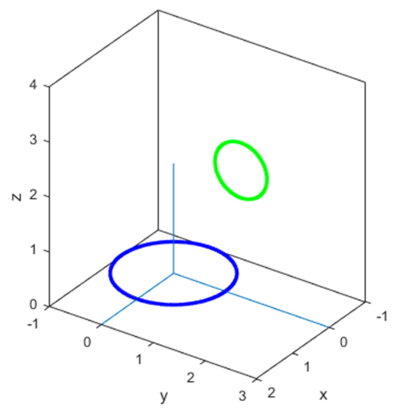
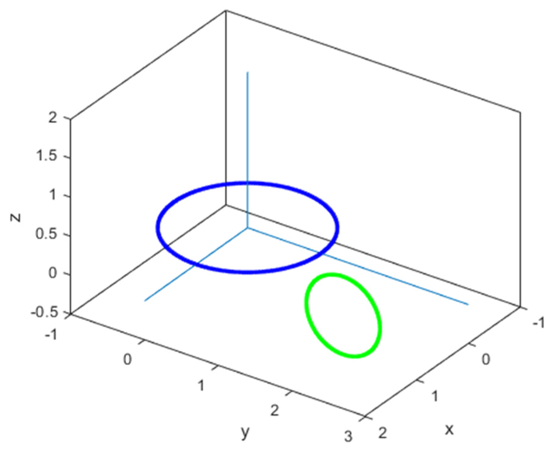
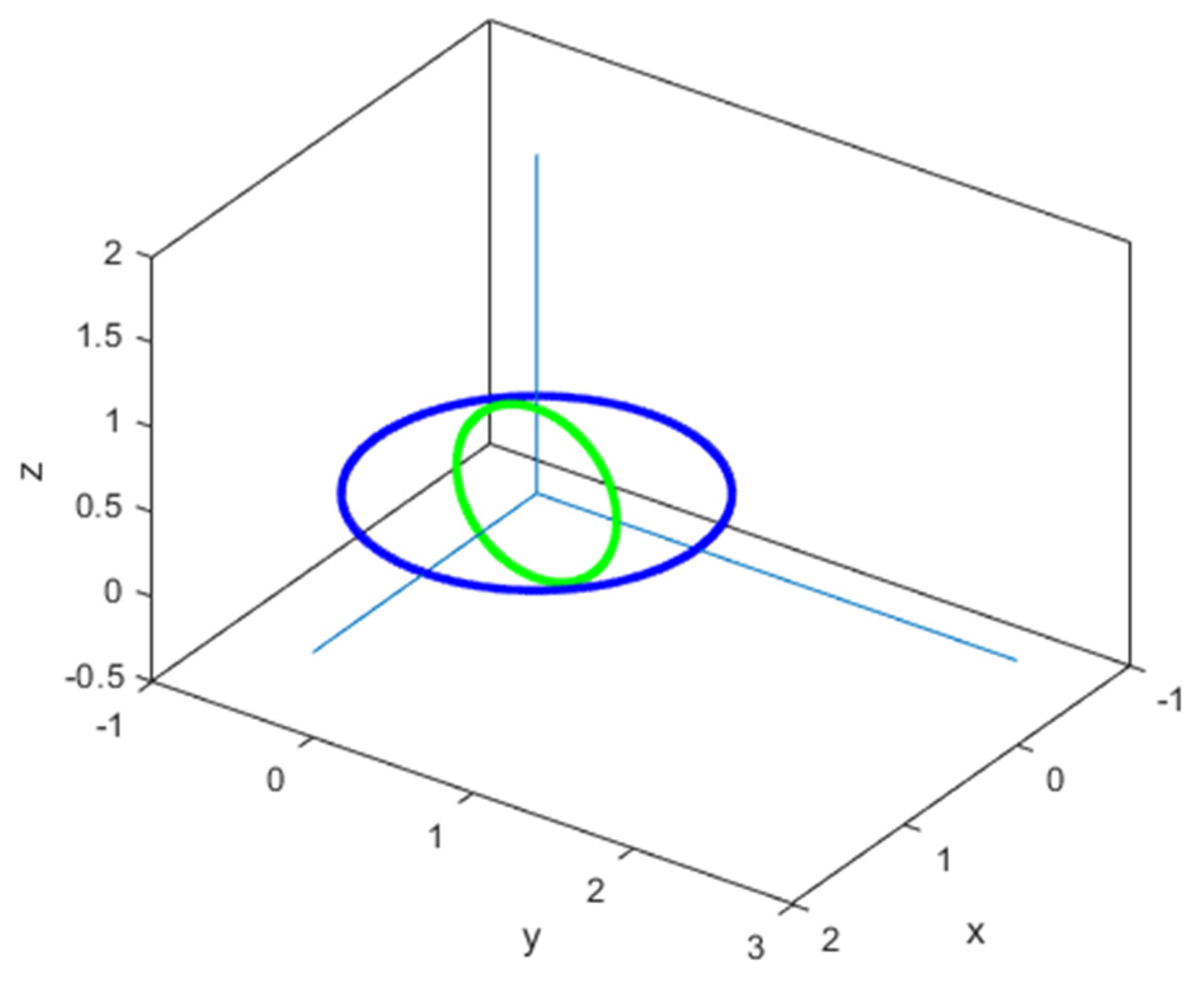
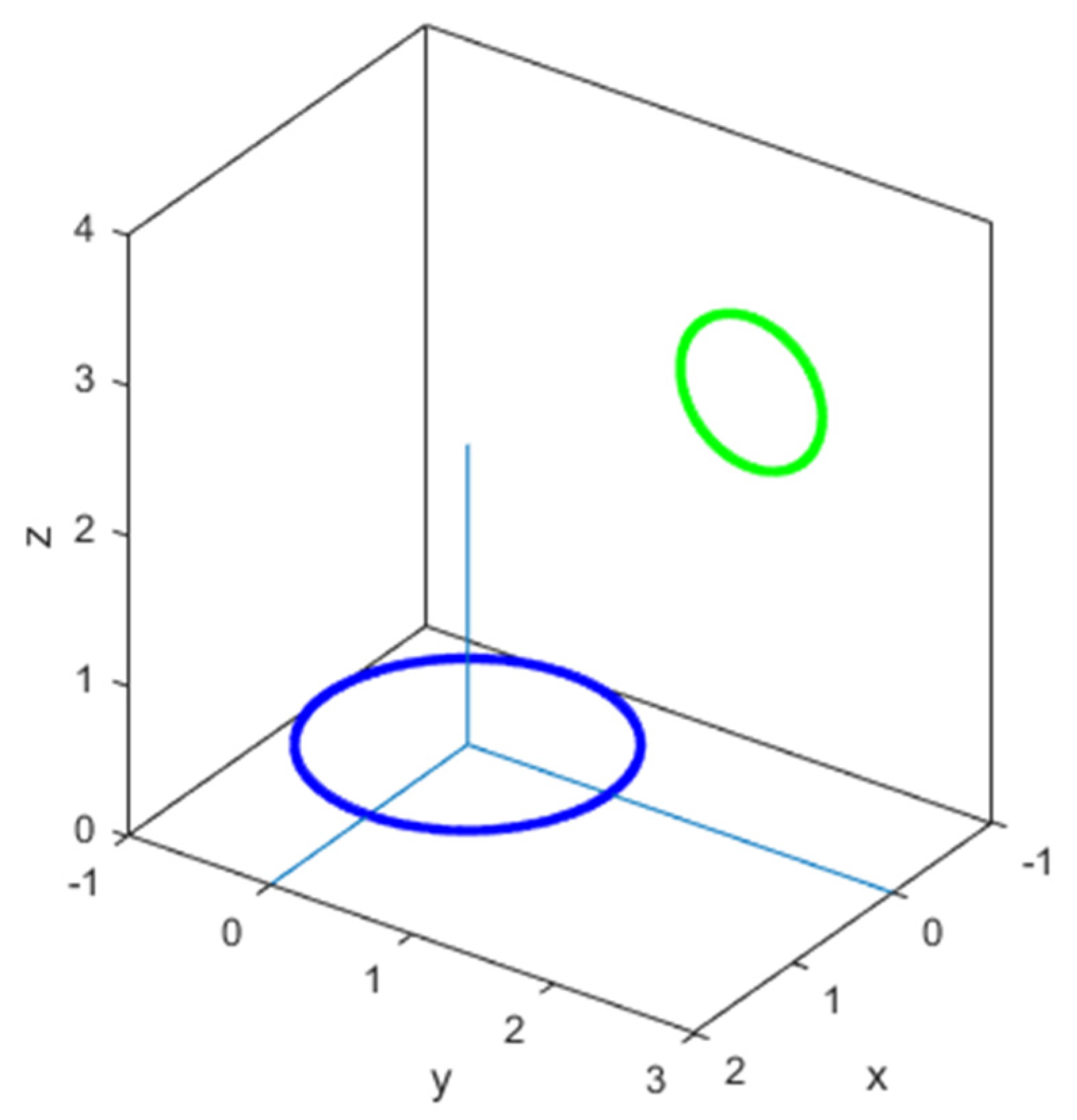
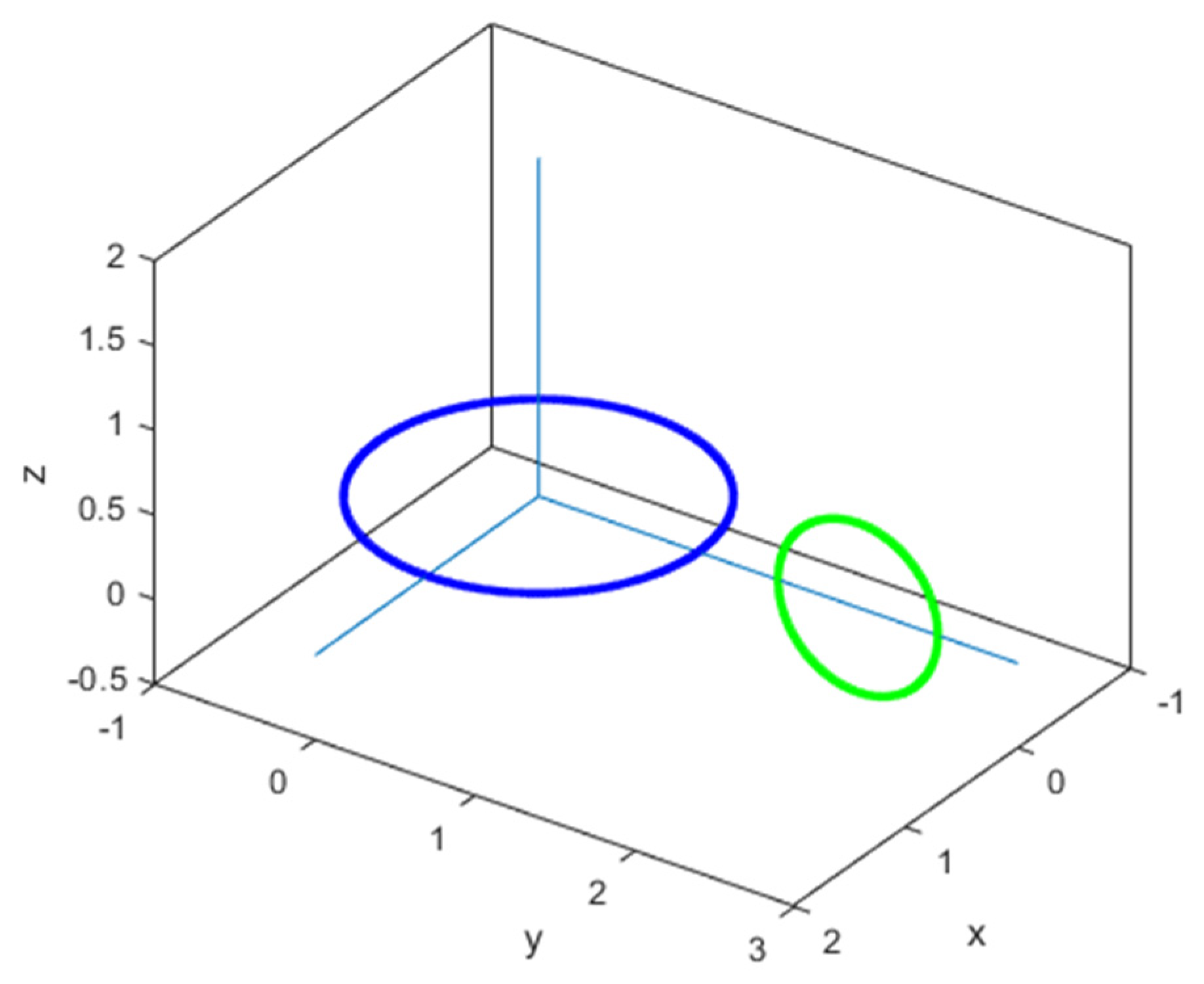
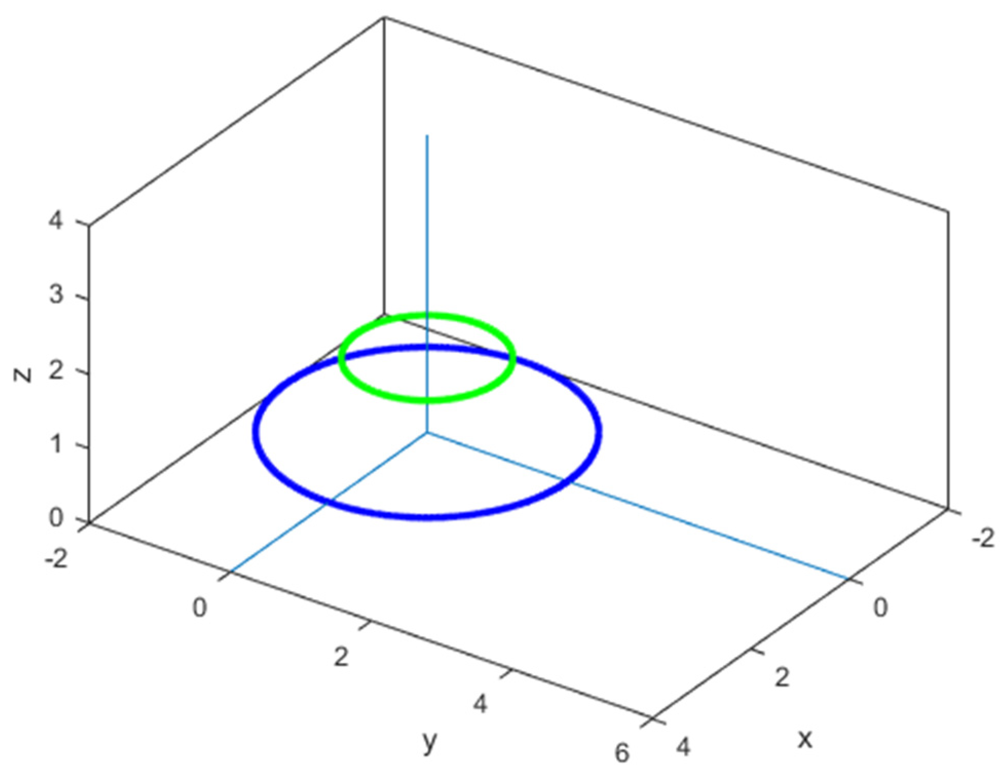
9. Numerical Validation

To verify the validity of the new formulas, the following set of examples are considered. The particular cases are discussed. The results obtained using the presented formulas are compared with those known in the literature.
Example 1. 
Calculate the magnetic vector potential produced by the current-carrying arc segment of the radius R P = 3 m at the point S ( x S , y S , z S ) = S (3 m, 4 m, 5 m). The current I P = 1 A.
Let us begin with the circular loop for which is φ1 = 0 and φ2 = 2π.
From Equations (16)–(18), one has the components, and the total magnetic vector potential as follows:
A x   S   = 28.61844373019504   nT · m , A y   S   = 21.46383279764628   nT · m , A z   S   = 0   T · m , A   S   = 35.7730546627438   nT · m .
From [11], one obtains the same results for the total magnetic vector potential.
Obviously, these are the known formulas for the current loop.
Let us take φ1 = π/3 and φ2 = 5π/4. From Equations (16)–(18), one finds:
A x   S   = 60.73902566793771   nT · m , A y   S   = 54.76725580732807   nT · m , A z   S   = 0   T · m , A   S   = 81.78436004368871   nT · m .
Thus, the analytic form of the magnetic vector potential is found for the different angle positions.
Example 2. 
Calculate the magnetic field produced by the current-carrying arc segment of the radius R P = 3 m at the point S ( x S , y S , z S ) = S (3 m, 4 m, 5 m). The current I P = 1 A.
Let us start with the circular loop for which is φ1 = 0 and φ2 = 2π.
From Equations (35)–(37), one finds the components, and the total magnetic field as follows:
B x   S   = 6.590422756026894   nT , B y   S   = 8.787230341369193   nT , B z   S   = 5.554432293082448   nT , B   S   = 12.30856641830695   nT .
The magnetic field produced by the circular loop can be considered as axisymmetric so that we need to calculate only the radial and azimuthal component. Applying equations from [11], these components as well as the total magnetic field are as follows:
B r   S   = 10.98403792671149   nT , B z   S   = 5.554432293082448   nT , B   S   = 12.30856641830695   nT .
From the previous calculations, the radial component of the magnetic field is:
B r   S   = B x 2   S   +   B y 2   S = 10.98403792671149   nT .
Thus, we show the validity of Equations (35)–(37).
From [11], we obtained the same results for the magnetic field. Obviously, these are the known formula for the current loop.
Now, let us apply these equations for the same problem but with the various positions of angles, for example, φ1 = π/6 and φ2 = 3π/4. We obtain:
B x   S   = 3.204077158320579   nT , B y   S   = 11.48651408884254   nT , B z   S   = 3.013457271456703   nT , B   S   = 12.29987971797063   nT .
Thus, these examples for the arbitrary angles may serve as the benchmark example. As one can see, the calculations of the magnetic vector potential and the magnetic field of the current-carrying segments with arbitrary angles are obtained in the closed form and expressed by the incomplete elliptic integrals of the first and the second kind. In the case of the circular loops, these calculations are the known and obtained over the complete elliptical integral of the first and the second kind. The analytical formula for the magnetic field is crucial for calculating other electromagnetic quantities such as the magnetic force, the magnetic torque, the mutual inductance, and the stiffness between inclined circular current-carrying arc segments.
Example 3. 
Calculate the magnetic force between two arc currying-courant segments whose radii are R P = 0.2 m and R S = 0.1 m, respectively. The first arc segment is placed in the plane XOY with the center at the origin and the second in the plane x + y + z = 0.3 with the center C (0.1 m; 0.1 m; 0.1 m). The currents are units.
We begin with two inclined circular loops; see Figure 3.
By using Ren’s method, [20], the components of the magnetic force are:
F x   = 0.10807277   μ N , F y   = 0.10807276   μ N F z = 1.4073547   μ N .
By using Poletkin’s method [31], the components of the magnetic force are as follows:
F x = 0.108072965612845   μ N , F y = 0.108072965612845   μ N , F z = 1.40737206031365   μ N .
From [25,26], the components of the magnetic force are:
F x = 0.1080729656128444   μ N , F y = 0.1080729656128444   μ N , F z = 1.407372060313649   μ N .
From the calculations, presented in this paper, using Equations (53)–(55), one has:
F x = 0.1080729656128444   μ N , F y = 0.1080729656128444   μ N , F z = 1.407372060313649   μ N .
Thus, the validity of the approach presented here is confirmed.
Figure 3. Two inclined circular loops. General case.
Physics 03 00067 g003
Now, let us apply these equations for the same problem but with the various positions of the segment angles, for example, φ1 = φ3 = π/6 and φ2 = φ4 = 3π/4. We obtain:
F x = 137.7416772905457   μ N , F y = 6.783844980209707   μ N , F z = 32.30984917651751   μ N .
Example 4. 
The center of the primary coil of the radius R P = 0.4 m is O (0; 0; 0) and the center of the secondary coil of the radius R S = 0.05 m is C (0.1 m; 0.15 m; 0.0 m). The secondary coil is in the plane 3x + 2y + z = 0.6. Calculate the magnetic force between coils. All currents are units. The angles of segments are, respectively, φ1 = 0, φ2 = 2π and φ3 = 0, φ4 = 19π/10, 195π/100, 19,999 π/10,000, 2π. Investigate four cases for angle φ4.
The first coil is the current loop. Using the method presented here, one has:
For φ4 = 19π/10,
F x = 1.030225970922242     nN , F y = 5.151227163000918   nN , F z = 27.14297688555945   nN .
For φ4 = 195π/100,
F x = 2.692181753461003   nN , F y = 1.173665675174731   nN , F z = 27.52894004960609   nN .
For φ4 = 19,999π/10,000,
F x = 4.171134702846683   nN , F y = 6.514234771668451   nN , F z = 27.71528704863114   nN .
For φ4 = 2π,
F x = 4.171776672650815   nN , F y = 6.523855691357912   nN , F z = 27.7154997521196   nN .
The last results for φ4 = 2π, are obtained in [25,26].
Thus, we show that the presented formulas for the magnetic force between two inclined current-carrying segments with arbitrary angels are correct which is proved by the limit case for the two inclined circular loops.
Example 5. 
The center of the primary coil of the radius R P = 0.3 m is O (0; 0; 0) and the center of the secondary coil of the radius R S = 0.3 m is C (0.1 m; −0.3 m; 0.2 m). The secondary coil is in the plane x − 2y + z = 0.9. All currents are units but of the opposite sign. The angles of segments are, respectively, φ1 = 0, φ2 = π, 3π/2, 7π/24, 90π/46, 1999π/1000, 2 π and φ3 = 0, φ4 = π, 3π/2, 7π/24, 90π/46, 1999π/1000, 2 π. Calculate the magnetic force between these current segments.
Using the presented method here, one finds:
φ1 = 0, φ2 = π, φ3 = 0, φ4 = π,
F x = 0.1434856008022091   μ N , F y = 0.1326852649109414   μ N , F z = 0.02679590119992052   μ N .
φ1 = 0, φ2 = 3π/2, φ3 = 0, φ4 = 3π/2,
F x = 0.125846805955475   μ N , F y = 0.1412059414594633   μ N , F z = 0.008568308516912724   μ N .
φ1 = 0, φ2 = 7π/4, φ3 = 0, φ4 = 7π/4,
F x = 0.1971372403346838   μ N , F y = 0.3359342255993592   μ N , F z = 0.1029523519216523   μ N .
φ1 = 0, φ2 = 90π/46, φ3 = 0, φ4 = 90π/46,
F x = 0.2298232863299166   μ N , F y = 0.5316472767567059   μ N , F z = 0.094553128442032   μ N .
φ1 = 0, φ2 = 1999π/1000, φ3 = 0, φ4 = 1999π/1000,
F x = 0.2292493650352244   μ N , F y = 0.5614719226361647   μ N , F z = 0.09253078729453428   μ N .
Let us take the limit case of two inclined current loops. This approach gives:
F x = 0.2292455704933025   μ N , F y = 0.5621415690326643   μ N , F z = 0.09249247340323912   μ N .
The last results are obtained in [25,26].
Thus, when the segments lead to the circular loops, we can see the results that converge to those of the circular loops.
Example 6. 
The center of the primary coil of the radius R P = 1 m is O (0; 0; 0) and the center of the secondary coil of the radius R S = 0.5 m is C (2 m; 2 m; 2 m). Coils have perpendicular axes (see Figure 4). The secondary coil is in the plane y = 2 m. Calculate the magnetic force between the coils. All currents are units.
This case is the singular case because a = c = 0. Let us begin with two perpendicular current loops [25,26], for which we found:
Figure 4. Two perpendicular circular loops. Singular case, a = c = 0, l = 0.
Physics 03 00067 g004
F x = 4.901398177052345   nN , F y = 1.984872313200137   nN , F z = 2.582265710169336   nN .
According to [20],
F x = 4.9013835   nN , F y = 1.9848816   nN , F z = 2.5821969   nN .
Using this paper, case 5.1.2 [ u =   1 , 0 , 0 , v =   0 , 0 , 1 ] and Equations (53)–(55), one has:
F x = 4.901398177052345   nN , F y = 1.984872313200137   nN , F z = 2.582265710169336   nN .
Using this paper, case 5.1.3 [ u =   0 , 0 , 1 , v =   1 , 0 , 0 ] and Equations (53)–(55) one has:
F x = 4.901398177052345   nN , F y = 1.984872313200137   nN , F z = 2.582265710169336   nN .
Thus, we obtained for case 5.1.3 the same results as in [25,26,31]. For case 5.1.2 we obtain the same results as in [25,26] but with opposite signs for each component, because in this case we did not take into consideration other unit vectors.
Let us take case 5.1.3. and φ1 = π/6, φ2 = 5π/6, φ3 = π/4, φ4 = 5π/4. The approach presented here gives:
F x = 12.06294047887778   nN , F y = 5.242872781049669   nN , F z = 7.708406091689127   nN .
Let us take case 5.1.3. and φ1 = π/1000, φ2 = 1999π/1000, φ3 = π/1000, φ4 = 1999π/1000. The approach presented here gives:
F x = 4.901398087973561   nN , F y = 1.977166719062928   nN , F z = 2.553525470247053   nN .
For φ1 = φ3 = 0 and φ2 = φ4 = 2π we approach the limit case (see the first calculation in this example).
Thus, this singular case, where the angles are arbitrary, can be used as the benchmark example which in the limit leads to the case of the perpendicular circular loops.
Example 7. 
Calculate the torque between two inclined current-carrying arc segments for which R P = 0.2 m and R S = 0.1 m. The first arc segment is placed in the plane XOY and the second in the plane x + y + z = 0.3 with center C (0.1 m; 0.1 m; 0.1 m). The currents are units.
Let us begin with two inclined circular loops for which φ1 = 0, φ2 = 2π, φ3 = 0 and φ4 = 2π (see Figure 3).
By using Ren’s method [20], the components of the magnetic torque are as follows:
τ x = 27.861249   nN · m , τ y = 27.861249   nN · m , τ z = 0   N · m .
By using Poletkin’s method [31], the components of the magnetic force are as follows:
τ x = 27.8620699713   nN · m , τ y = 27.8620699713   nN · m , τ z = 5.65233285126159 × 10 14   0   N · m .
Using the approach presented in this paper, Equations (59)–(61), one finds:
τ x = 27.86206997129496   nN · m , τ y = 27.86206997129496   nN · m , τ z = 5.007385868157401 × 10 64   0   N · m .
All the results are in an excellent agreement. Thus, the validity of the approach presented here is confirmed.
Let us take φ1 = π/12, φ2 = π, φ3 = 0 and φ4 = 2π.
The approach presented here gives:
τ x = 0.4295228631728361   nN · m , τ y = 0.3155545746006545   nN · m , τ z = 0.1139682885721816   nN · m .
As it was mentioned above, the magnetic torque calculation represents novelty in the literature.
Example 8. 
Let us consider two arc segments of the radii R P = 1 m and R S = 0.5 m. The primary loop lies in the plane z = 0 m, and it is centered at O (0 m; 0 m; 0 m). The secondary loop lies in the plane x = 1 m, with its center located at C (1 m; 2 m; 3 m). Calculate the torque between these inclined coils. All currents are units. Investigate the point (a) C (1 m; 2 m; 3 m), (b) C (1 m; 2 m; 0 m), (c) C (1 m; 0 m; 0 m), (d) C (0 m, 0 m, 0 m).
Obviously, these coils are perpendicular (see Figure 5, Figure 6, Figure 7 and Figure 8) but by the presented method these cases are the not singular case because a = 1, b = c = 0 (L = l = 1).
Let us take into configuration two perpendicular loops. The approach presented here gives:
Figure 5. Case (a): two perpendicular circular loops. Not a singular case, (a = 1, b = c = 0, L = l = 1).
Physics 03 00067 g005
Figure 6. Case (b): two perpendicular circular loops. Not a singular case, (a = 1, b = c = 0, L = l = 1).
Physics 03 00067 g006
Figure 7. Case (c): two perpendicular circular loops. Not a singular case, (a = 1, b = c = 0, L = l = 1).
Physics 03 00067 g007
Figure 8. Case (d): two perpendicular circular loops. Not a singular case, (a = 1, b = c = 0, L = l = 1).
Physics 03 00067 g008
(a)
C (1 m; 2 m; 3 m)
By the presented method,
τ x = 0   N · m , τ y = 4.668729435430873   nN · m , τ z = 5.739664477343296   nN · m .
According to [20],
τ x = 4.1994108 × 10 14 0   N · m , τ y = 4.6686544   nN · m , τ z = 5.7396408   nN · m .
In [31], this case is the singular case for which we have:
τ x = 2.858735873626482 × 10 25 0   N · m , τ y = 4.668669979976015   nN · m , τ z = 5.739664477343291   nN · m .
(b)
C (1 m; 2 m; 0 m)
By the presented method,
τ x = 0   N · m , τ y = 27.83604705327234   nN · m , τ z = 1.527368681710413 × 10 146 0   N · m .
By [20],
τ x = 1.5403435 × 10 16 0   N · m , τ y = 27.835798   nN · m , τ z = 1.3063032 × 10 11   N · m .
In [31], this case is the singular for which we have:
τ x = 1.704466532265166 × 10 24   0   N · m , τ y = 27.83605090793333   nN · m , τ z = 0   N · m .
(c)
C (0 m; 0 m; 0 m)
By the presented method,
τ x = 0   nN , τ y = 185.0045402475441   nN · m , τ z = 7.657062549408825 × 10 138 0   nN · m .
According to [20],
τ x = 1.6956645 × 10 14 0   N · m , τ y = 184.99891   nN · m , τ z = 2.2736774 × 10 12   N · m .
In [31], this case is the singular for which we have:
τ x = 1.132826091097256 × 10 24   0   N · m , τ y = 185.0045403925399   nN · m , τ z = 0   N · m .
(d)
C (1 m; 0 m; m)
By the presented method,
τ x = 0   N · m , τ y = 435.2765381474917   nN · m , τ z = 3.403343626298156 × 10 128 0   N · m .
According to [20],
τ x = 4.3207387 × 10 20 0   N · m , τ y = 435.27404   nN · m , τ z = 5.5087283 × 10 13   N · m .
In [31], this case is the singular for which we have:
τ x = 2.665551203021357 e × 10 23 0   N · m , τ y = 435.3175470473964   nN · m , τ z = 0   N · m .
All the results are in exceptionally good agreement. We state that the presented method is exact. In [2], the authors use the small segments to approximate the circular loops. In [31], this case is singular as previously mentioned.
Example 9. 
Let us consider two arc segments of the radii R P = 1 m and R S = 0.5 m. The primary loop lies in the plane z = 0 m, and it is centered at O (0 m; 0 m; 0 m). The secondary loop lies in the plane x = 0 m, with its center located at C (0 m; 2 m; 3 m). Calculate the torque between these inclined coils. All currents are units. Investigate the point (a) C (0 m; 2 m; 3 m), (b) C (0 m; 2 m; 0 m), (c) C (0 m; 0 m; 3 m), (d) C (0 m; 0 m; 0 m).
Obviously, these coils are perpendicular (see Figure 9, Figure 10, Figure 11 and Figure 12) but according to the presented method these cases are not singular cases because a = 1, b = c = 0, (L = l = 1). In [31] this case is the singular case, and it was studied with special attention. Grover’s formula A.8 given in [2] was corrected to obtain the correct results for this singular case.
(a)
C (0 m; 2 m; 3 m)
By the presented method,
τ x = 0   N · m , τ y = 6.03647173178846   nN · m , τ z = 6.860953527497661   nN · m .
According to [31] we obtain.
τ x = 0   N · m , τ y = 6.036471731788459   nN · m , τ z = 6.860953527497644   nN · m .
(b)
C (0 m; 2 m; 0 m)
By the presented method,
τ x = 0   N · m , τ y = 46.60910437567855   nN · m , τ z = 1.027871789475573 × 10 136 0   N · m .
According to [31], we obtain:
τ x = 2.853984524239991 × 10 24   0   N · m . τ y = 46.6091043756787   nN · m , τ z = 1.282404413152518 × 10 23 0   N · m .
(c)
C (0 m; 0 m; 3 m)
By the presented method,
τ x = 0   N · m , τ y = 16.3969954478874   nN · m , τ z = 1.682963244063953 × 10 128 0   N · m .
According to [31], we obtain:
τ x = 7.300027041557918 × 10 18 0   N · m , τ y = 16.39567517228915   nN · m . τ z = 1.682963244063953 × 10 9 0   N · m .
(d)
C (0 m; 0 m; 0 m)
By the presented method,
τ x = 0   N · m , τ y = 435.2765381474917   nN · m , τ z = 1.731874227122655 × 10 128 0   N · m .
According to [31], we have:
τ x = 2.66513932049866 × 10 23 0   N · m , τ y = 435.2502815267608   nN · m , τ z = 5.416141293918174 × 10 16 0   N · m .
Thus, we investigated all possible cases in this example where the coils are the perpendicular, but the general formula for the torque treats this case (b = c = 0) as the regular case but in [31] it is the singular case. All the results are in excellent agreement.
Example 10. 
Let us consider two arc segments of the radii R P = 40 cm and R S = 10 cm. The primary arc segment lies in the plane z = 0 cm, and it is centered at O (0 cm;0 cm; 0 cm). The secondary arc segment lies in the plane y = 20 cm, with its center located at C (0 cm; 20 cm; 10 cm). Calculate the torque between two arc segments with φ1 = 0, φ2 = π, φ3 = 0, φ4 = π.
This case is the singular case because a = c = 0. Let us begin with two inclined circular loops (see Figure 4).
Using case 6.1.2 [ u =   1 , 0 , 0 , v =   0 , 0 , 1 ] and Equations (59)–(61), one has:
τ x = 0.498395165432447   nN · m , τ y = 0   N · m , τ z = 3.696785155039511 × 10 137 0   N · m .
Using case 6.1.3 [ u =   0 , 0 , 1 , v =   1 , 0 , 0 ] and Equations (59)–(61), one has:
τ x = 0.498395165432447   nN · m , τ y = 0   N · m , τ z = 3.696785155039511 × 10 137   0   N · m .
Thus, we obtained the same results with case 6.1.3 and case 6.1.2 but with opposite signs for each component. This was explained in the previous examples, where the singularities appear.
Let us take case 6.1.2. and φ1 = 0, φ2 = π, φ3 = 0, φ4 =2 π. The approached here gives:
τ x = 24.91975827162235   nN · m , τ y = 0     N · m , τ z = 0.9803004730404883   nN · m .
Let take us case 6.1.3. and φ1 = 0, φ2 = π, φ3 = 0, φ4 =2 π. The approach here gives:
τ x = 24.91975827162235   nN · m , τ y = 0   N · m , τ z = 0.9803004730404883   nN · m .
These results were expected.
Example 11. 
The center of the primary coil of the radius R P = 1 m is O (0 m; 0 m; 0 m) and the center of the secondary coil of the radius R S = 0.5 m is C (2 m; 2 m; 2 m). The secondary coil is in the plane y = 2 m which means that the coils are with perpendicular axes. Calculate the magnetic torque between coils for which is φ1 = 0, φ2 = π, φ3 = π and φ4 = 2π. All currents are units.
This case is the singular case because a = c = 0. Let us start with two perpendicular current loops, (see Figure 4).
Using case 6.1.2 [ u =   1 , 0 , 0 , v =   0 , 0 , 1 ] and Equations (59)–(61), one finds:
τ x = 0.3526562725465321   nN · m , τ y = 0   N · m , τ z = 5.833051727704416   nN · m .
Using case 6.1.3 [ u =   0 , 0 , 1 , v =   1 , 0 , 0 ] and Equations (59)–(61), one finds:
τ x = 0.3526562725465321   nN · m , τ y = 0   N · m , τ z = 5.833051727704416   nN · m .
Thus, we obtained the same results with case 6.1.3 and case 6.1.2 but with opposite signs for each component.
By [20],
τ x = 0.35628169   nN · m , τ y = 0.40169339 × 10 15 0   N · m , τ z = 5.8330053   nN · m .
All the results are in excellent agreement.
For φ1 = 0, φ2 = π, φ3 = π and φ4 =2π:
Using case 6.1.2 [ u =   1 , 0 , 0 , v =   0 , 0 , 1 ] and (59)–(61), one has:
τ x = 7.24520528470814   nN · m , τ y = 0   N · m . τ z = 3.767244177134524   nN · m .
Using case 6.1.3 [ u =   0 , 0 , 1 , v =   1 , 0 , 0 ] and Equations (59)–(61), one has:
τ x = 7.245205284708146   nN · m , τ y = 0   N · m . τ z = 3.767244177134524   nN · m .
Thus, we obtained the same results with case 6.1.3 and case 6.1.2 but with opposite signs for each component that was proved in previous singular cases.
Example 12. 
Calculate the mutual inductance between two inclined current-carrying arc segments for which is R P = 0.2 m and R S = 0.1 m. The first arc segment is placed in the plane XOY and the second in the plane x + y + z = 0.3 with the center C (0.1 m; 0.1 m;0.1 m) which lies within.
Let us begin with φ1 = 0, φ2 = 2π, φ3 = 0 and φ4 = 2π (see Figure 3).
Applying Equation (64), the mutual inductance for inclined circular loops is:
M = 81.31862021231823   nH .
We find the same result in [24].
Now, let us change the positions of the arc segments, for example, φ1 = 0, φ2 = π/2, φ3 = π and φ4 = 3π/2. Applying Equation (63), the mutual inductance is:
M = 17.38258810896817   nH .
Example 13. 
Let us consider two arc segments of the radii R P = 40 cm and R S = 10 cm. The primary arc segment lies in the plane z = 0 cm, and it is centered at O (0 cm; 0 cm; 0 cm). The secondary arc segment lies in plane y = 20 cm, with its center is located at C (0 cm; 20 cm; 10 cm). Calculate the mutual inductance between two arc segments.
This is the singular case, a = c = 0. Let us begin with two circular loops for which is φ1 = 0, φ2 = 2π, φ3 = 0 and φ4 =2π, (see Figure 4).
M = 10.72715167866112   nH .
We find the same result in [24].
For y = 20 cm the mutual inductance is:
M = 10.72715167866112   nH .
For y = 0 cm the mutual inductance is:
M = 0   H .
This result is found in [30].
Example 14. 
Let us consider two arc segments of the radii R P = 40 cm and R S = 10 cm, which are mutually perpendicular to each other. The primary arc segment lies in the plane z = 0 m, and it is centered at O (0 m; 0 m; 0 m), and the center of the secondary coil is located at origin, thus C = O (0;0;0). Calculate the mutual inductance between two arc segments, [30].
Let us begin with two circular loops for which is φ1 = 0, φ2 = 2π, φ3 = 0 and φ4 = 2π.
Here, we taste tree cases (1) a = 1, b = c = 1; (2) a = 0, b = 1, c = 0; (3) a = b = 0, c = 1.
For all cases, the mutual inductance [24] gives:
M = 0   H .
From this paper calculations, we obtained the same value. This means that for any position of the secondary loop the mutual inductance is zero when the center of the second loop is positioned in the origin O. The same results are obtained in [30].
Example 15. 
Let us consider the previous example, but the center of the secondary coil is at the plane XOY with the following coordinates x C = y C = 10 cm and z C = 0 cm, [30]. Calculate the mutual inductance between these coils.
From this approach the mutual inductance gives:
M = 1.78729016039874 × 10 143 0   H .
In [30], the mutual is found to be zero.
Example 16. 
Calculate the stiffness between two coaxial circular loops for which is R P = 2 m, and R S = 1 m. The axial distance between loops is 1 m.
Let us begin with two parallel loops (see Figure 13) for which φ1 = 0, φ2 = 2π, φ3 = 0 and φ4 = 2π.
Obviously, there is only the stiffness kzz and other stiffnesses are zero because of the coaxial loops.
From Equation (75), the stiffness is:
k z z = F z z = 0.2064021172440473 × 10 6   N / m .
From developed general Formula (76),
k z z = F z z = 0.2064021172440473 × 10 6   N / m .
Thus, with the benchmark formula we confirmed the validity of the general formula for kzz.
Example 17. 
Calculate the stiffness between two inclined current-carrying arc segments (see Figure 3) for which R P = 0.2 m and R S = 0.1 m. The first arc segment is placed in the plane XOY and the second in the plane x + y + z = 0.3 with the center C (0.1 m; 0.1 m; 0.1 m) which lies in this plane.
Let us begin with two circular loops for which φ1 = 0, φ2 = 2π, φ3 = 0 and φ4 = 2π.
From this approach (76), one has:
k z z = F z z = 57.36862305837861 × 10 6   N / m .
This example could be used as the benchmark example to test other methods in which the axial stiffness is calculated. Now, let us take φ1 = π/4, φ2 = π/2, φ3 = 3π/4 and φ4 = 3π/2.
From Equation (76), one has:
k z z = F z z = 28.70523534358855 × 10 6   N / m .
Example 18. 
Let us consider two arc segments of the radii R P = 40 cm and R S = 10 cm. The primary arc segment lies in the plane z = 0 cm, and it is centered at O (0 cm; 0 cm; 0 cm). The secondary arc segment lies in the plane y = 20 cm, with its center is located at C (10 cm; 20 cm; 10 cm). Calculate the stiffness between two arc segments.
This case is the singular case because a = c = 0. Let us start with two perpendicular current circular loops (see Figure 4).
Using case 8.1.2 [ u =   1 , 0 , 0 , v =   0 , 0 , 1 ] and Equation (76), one finds:
k z z = 1.322488731905245   μ N / m .
Using case 8.1.3 [ u =   0 , 0 , 1 , v =   1 , 0 , 0 ] and Equation (76) one finds:
k z z = 1.322488731905245   μ N / m .
Thus, we obtained with case 8.1.2 and case 8.1.3 the same results but with opposite signs for each component.
Now, let us take φ1 = π, φ2 = 2π, φ3 = π and φ4 = 2π.
Using case 8.1.2 [ u =   1 , 0 , 0 , v =   0 , 0 , 1 ] and Equation (76), one has:
k z z = 34.21629087092779   μ N / m .
Using case 8.1.3 [ u =   0 , 0 , 1 , v =   1 , 0 , 0 ] and Equation (76), one has:
k z z = 34.21629087092779   μ N / m .
These results were expected.

10. Conclusions

In this paper, we give some ameliorated and new formulas for calculating important electromagnetic quantities such as the magnetic vector potential, the magnetic field, the magnetic force, the mutual inductance, and the stiffness between two inclined current-carrying arc segments in air. The angles of arc segments are arbitrary. All formulas are developed in the close form over the incomplete elliptic integrals of the first and the second kind (the magnetic vector potential and the magnetic field) and in the simple integral form whose kernel functions are also given in the close form over the incomplete elliptic integrals of the first and the second kind (the magnetic force, the magnetic torque, the mutual inductance, and the stiffness). The magnetic vector potential and the magnetic field calculations are given in the analytical form expressed by the incomplete elliptic integrals of the first and second kind. All particular cases are included. Even though these calculations exist in the literature, those presented here, where the angles of coils are arbitrary, present the ameliorated and simplified formulas which are easy to use. The formulas for calculation of the magnetic force and the mutual inductance are significantly simplified regarding those known in the literature. Singular cases are included. Finally, the formulas for calculating the magnetic torque and the stiffness between inclined circular loops or segments appear for the first time in this form in the literature. All electromagnetic quantities are given in quite simple form so that potential readers can easily program them in MATLAB or Mathematica. Many examples confirmed the validity of the presented formulas for inclined circular current-carrying arc segments, and they can be used as the benchmark examples for testing other methods concerning this subject.

Funding

This research received no external funding.

Acknowledgments

The author thanks Y. Ren of the Hefei Institute of Plasma Physics, Chinese Academy of Science, Anhui China, and K.V. Poletkin of Innopolis University, Innopolis, Russia for their extremely useful comments and suggestions and for providing extremely high precision calculations for the magnetic force and the torque between inclined circular loops which has proven invaluable in validating the method presented here.

Conflicts of Interest

The author declares no conflict of interest.

Appendix A

I 1 = β 1 β 2 sin γ 2 β Δ d β = sin γ β 1 β 2 cos 2 β Δ d β cos γ β 1 β 2 sin 2 β Δ d β = y S p β 1 β 2 1 2 sin 2 β Δ d β 2 x S p β 1 β 2 sin β cos β Δ d β .
From [39,40] we obtain the final expression in the analytical form,
I 1 = 1 p k 2   y S   k 2 2 F   β , k   +   2 E   β , k   +   2 x S Δ   β 2     β 1 , I 2 = β 1 β 2 cos γ 2 β Δ d β = cos γ β 1 β 2 cos 2 β Δ d β   +   sin γ β 1 β 2 sin 2 β Δ d β = x S p β 1 β 2 1 2 sin 2 β Δ d β   +   2 y S p β 1 β 2 sin β cos β Δ d β , I 2 = 1 p k 2   x S   k 2 2 F   β , k   +   2 E   β , k   2 y S Δ   β 2     . β 1

Appendix B

I 3 = β 1 β 2 cos γ 2 β r P S 3 d β =   cos γ β 1 β 2 cos 2 β r T P 3 d β   +   sin γ β 1 β 2 sin 2 β r T P 3 d β   = x S p β 1 β 2 1 2 sin 2 β Δ 3 d β   +   y S p β 1 β 2 sin 2 β Δ 3 d β = x s p k 2   1 k 2   k 2 2 E   β , k   +   2 2 k 2 F   β , k   +   k 2 ( 2 k 2 ) k 2 ( 2 k 2 ) sin β cos β Δ β 2     , β 1 I 3 = x s p k 2   1 k 2   k 2 2 E   β , k   +     2 2 k 2 F   β , k   +   k 2 ( 2 k 2 ) sin β cos β Δ β 2     β 1   +   2 y S p k 2 Δ β 2     . β 1 I 4 = β 1 β 2 sin γ 2 β r P S 3 d β     sin γ β 1 β 2 cos 2 β r T P 3 d β cos γ β 1 β 2 sin 2 β r T P 3 d β   = y s p k 2   1 k 2     k 2 2 E   β , k   +     2 2 k 2 F   β , k   +   k 2 ( 2 k 2 ) sin β cos β Δ β 2     β 1 2 x S p k 2 Δ β 2     . β 1 I 5 = β 1 β 2 R P   +   x S 2   +   y S 2 cos 2 β Δ 3 d β = β 1 β 2 R P   +   p   Δ 3 d β 2 p β 1 β 2 cos 2 β Δ 3 d β = 1 k 2   1 k 2 k 2   R p   +   p     2 p E   β , k   +     2 p 2 p k 2 F   β , k   +   k 2 ( 2 p   R p   +   p k 2 ) sin β cos β Δ β 2     . β 1

Appendix C

I 6 = φ 1 φ 2 l S x sin t   +   l S y cos t x S 2   +   y S 2   +   z S 2   +   R P 2 2 R P x S 2   +   y S 2 cos t γ d t .
The substitution t γ = π 2 β gives,
I 6 = 2 l x S   R P   +   x S 2   +   y S 2 2   +   z S 2 sin γ β 1 β 2 cos 2 β Δ d β cos γ β 1 β 2 sin 2 β Δ d β   +   2 l y S   R P   +   x S 2   +   y S 2 2   +   z S 2 cos γ β 1 β 2 cos 2 β Δ d β   +     sin γ β 1 β 2 sin 2 β Δ d β = l x S k p R P p   y S β 1 β 2 1 2 sin 2 β Δ d β 2 x S β 1 β 2 sin β cos β Δ d β   +   l y S k p R P p   x S β 1 β 2 1 2 sin 2 β Δ d β   +   2 y S β 1 β 2 sin β cos β Δ d β = l S y k p R P p l y s x S l x s   y S     k 2 2 F   β , k   +   2 E   β , k β 2 β 1 2 Δ l y s y S   +   l x s   x S β 2 β 1 .

Appendix D

k z z = F z z s = I S R S z s φ 3 φ 4 l x S B y   S   l y S B x   S d θ = I S R S φ 3 φ 4 l x S z s B y   S   +   l x S B y   S z s l y S z s B x   S   l y S B x   S z s d θ = I S R S φ 3 φ 4 l x S B y   S z s l y S B x   S z s d θ = b e c a u s e     l x S z s = l y S z s = 0 = μ 0 I P I S R S 16 π R P φ 3 φ 4 l x S   z s k   1     k 2 p 5 2   I y y z s l y S   z s k   1     k 2 p 5 2   I x x z s d θ = μ 0 I P I S R S 16 π R P φ 3 φ 4 k   1 k 2 p 5 2 l x S T z z 1 l y S T z z 2 d θ . T z 1 = z s z s k   1 k 2   I y y = k   1 k 2   I y y   +   k k   1 k 2 k z s I y y   +   z s k   1 k 2 I y y z s k z s = z s k 3 4 p R P , T z 1 = k   1 k 2 T z z 1 , T z z 1 = c 1 I y y   +   z S   I y y z s , T z z 2 = c 1 I x x   +   z S   I x x z s .
I x x and I y y are given in (76) and (77).
c 1 = 1 z S 2   k 2 4 p R P 1   +   k 2 1 k 2 ,   I y y z s = z s   y S   A 2 A 1   2 x S   1 k 2   Δ 2 1 Δ 1 1   = y S z s   A 2 A 1 x S z S p R P k 4   Δ 2 1 Δ 1 1   +   x S z S 2 p R P k 4   1 k 2 sin 2 β 2 Δ 2 3 sin 2 β 1 Δ 1 3 . A 2 z s = 2 k E   β 2 , k k z s   +     k 2 2 d E   β 2 , k d k k z s   +     2 2 k 2 F   β 2 , k k z s 4 k d F   β 2 , k d k k z s   +   sin 2 β 2 2 k z s 4 k   1 k 2 1 Δ 2   +   k 3   2 k 2 sin 2 β 2 Δ 2 3 = k z s 2 k E   β 2 , k     2 F   β 2 , k   +     k 2 2 d E   β 2 , k d k   +     2 2 k 2 d F   β 2 , k d k   +   k sin 2 β 2 2 Δ 2 4   1 k 2   +   k 2   2 k 2 sin 2 β 2 Δ 2 2 . A 1 z s = A 2   β 2 β 1 , k z s   .   I y y z s = y S   b 1   +   2 x S   b 2 . b 1 = 3 E   β , k   F   β , k β 2 β 1   +   sin 2 β Δ   1 2 k 2   +   sin 2 β sin 2   β Δ 3 k 2   2 k 2 2 β 2 β 1 . b 2 = 2 Δ β 2 β 1   1 k 2 sin 2 β Δ 3 β 2 β 1 . T z z 1 = I y y =   +   z S   I x x z s T z z 1 = I y y z S 2 k 3 p R P 1   +   k 2 1 k 2 I y y z S 2 k 4 p R P   I y y z s .
Similarly,
T z z 2 = I x x z S 2 k 3 p R P 1   +   k 2 1 k 2 I x x z S 2 k 4 p R P   I x x z s ,   I x x z s = x S   b 1 2 y S b 2 .

References

  1. Maxwell, J.C. A Treatise on Electricity and Magnetism, 3rd ed.; Dover Publications Inc.: New York, NY, USA, 1954; Volume 2. [Google Scholar]
  2. Grover, F.W. Inductance Calculations; Dover: New York, NY, USA, 1964; Chapters 2 and 13. [Google Scholar]
  3. Snow, C. Formulas for Computing Capacitance, and Inductance; National Bureau of Standards Circular 544: Washington, DC, USA, 1954.
  4. Kalantarov, P.L. Inductance Calculations; National Power Press: Moscow, USSR, 1955. (In Russian) [Google Scholar]
  5. Kalantarov, P.L.; Zeitlin, L.A. Raschet Induktivnostey [Calculation of Inductances]; Energoatomizdat: Leningrad, USSR, 1986. (In Russian) [Google Scholar]
  6. Urankar, L. Vector potential and magnetic field of current-carrying finite arc segment in analytical form, part I: Filament approximation. IEEE Trans. Magn. 1980, 16, 1283–1288. [Google Scholar] [CrossRef]
  7. Urankar, L. Vector potential and magnetic field of current-carrying finite arc segment in analytical form, part II: Thin sheet approximation. IEEE Trans. Magn. 1982, 18, 911–917. [Google Scholar] [CrossRef]
  8. Urankar, L. Vector potential and magnetic field of current-carrying finite arc segment in analytical form, part III: Exact computation for rectangular cross section. IEEE Trans. Magn. 1982, 18, 1860–1867. [Google Scholar] [CrossRef]
  9. Urankar, L. Vector potential and magnetic field of current-carrying finite arc segment in analytical form, part IV: General three-dimensional current density. IEEE Trans. Magn. 1984, 20, 2145–2150. [Google Scholar] [CrossRef]
  10. Urankar, L. Vector potential and magnetic field of current-carrying circular finite arc segment in analytical form. V. Polygon cross section. IEEE Trans. Magn. 1990, 26, 1171–1180. [Google Scholar] [CrossRef]
  11. Walstrom, P.L. Algorithms for Computing the Magnetic Field, Vector Potential, and Field Derivatives for Circular Current Loops in Cylindrical Coordinates; National Laboratory: Los Alamos, NM, USA, 2017. [CrossRef]
  12. Christodoulides, C. Comparison of the Ampere and Biot-Savart magnetostatic force laws in their line-current-element forms. Am. J. Phys. 1988, 56, 357–362. [Google Scholar] [CrossRef]
  13. Babic, S.; Krstajic, B.; Milojkovic, S.; Andjelic, Z. Magnetostatic Field of Thin Current-Carrying Arc Filament. In Proceedings of the Fifth International Symposium on High Voltage Engineering, Braunshweige, Germany, 24–28 August 1987. [Google Scholar]
  14. Smith, M.; Fokas, N.; Hart, K.; Babic, S.I.; Selvaggi, J.P. The magnetic field produced from a conical current sheet and from a thin and tightly wound conical coil. Prog. Electromagn. Res. B 2021, 90, 1–20. [Google Scholar] [CrossRef]
  15. Conway, J. Exact solutions for the magnetic fields of axisymmetric solenoids and current distributions. IEEE Trans. Magn. 2001, 37, 2977–2988. [Google Scholar] [CrossRef]
  16. Conway, J.T. Trigonometric Integrals for the magnetic field of the coil of rectangular cross section. IEEE Trans. Magn. 2006, 42, 1538–1548. [Google Scholar] [CrossRef]
  17. Conway, J.T. Inductance calculations for circular coils of rectangular cross section and parallel axes using bessel and struve functions. IEEE Trans. Magn. 2009, 46, 75–81. [Google Scholar] [CrossRef]
  18. Ren, Y.; Wang, F.; Kuang, G.; Chen, W.; Tan, Y.; Zhu, J.; He, P. Mutual inductance and force calculations between coaxial bitter coils and superconducting coils with rectangular cross section. J. Supercond. Nov. Magn. 2010, 24, 1687–1691. [Google Scholar] [CrossRef]
  19. Ren, Y.; Zhu, J.; Gao, X.; Shen, F.; Chen, S. Electromagnetic, mechanical, and thermal performance analysis of the CFETR magnet system. Nucl. Fusion 2015, 55, 093002. [Google Scholar] [CrossRef]
  20. Wang, Z.J.; Ren, Y. Magnetic force and torque calculation between circular coils with nonparallel axes. IEEE Trans. Appl. Supercond. 2014, 24, 4901505. [Google Scholar] [CrossRef]
  21. Babic, S.I.; Akyel, C. Torque calculation between circular coils with inclined axes in air. Int. J. Numer. Model. Electron. Netw. Devices Fields 2011, 24, 230–243. [Google Scholar] [CrossRef]
  22. Babic, S.; Akyel, C. New formulas for calculating torque between filamentary circular coil and thin wall solenoid with inclined axes whose axes are at the same plane. Prog. Electromagn. Res. M 2018, 73, 141–151. [Google Scholar] [CrossRef]
  23. Babic, S.; Akyel, C. Magnetic force between inclined circular filaments placed in any desired position. IEEE Trans. Magn. 2011, 48, 69–80. [Google Scholar] [CrossRef]
  24. Babic, S.; Sirois, F.; Akyel, C.; Girardi, C. Mutual inductance calculation between circular filaments arbitrarily positioned in space: alternative to Grover’s formula. IEEE Trans. Magn. 2010, 46, 3591–3600. [Google Scholar] [CrossRef]
  25. Babic, S.I.; Akyel, C. Magnetic force calculation between thin coaxial circular coils in air. IEEE Trans. Magn. 2008, 44, 445–452. [Google Scholar] [CrossRef]
  26. Babic, S.I.; Akyel, C. Magnetic force between inclined circular loops (Lorentz approach). Prog. Electromagn. Res. B 2012, 38, 333–349. [Google Scholar] [CrossRef] [Green Version]
  27. Ravaud, R.; Lemarquand, G.; Lemarquand, V. Force and stiffness of passive magnetic bearings using permanent magnets. Part 1: Axial magnetization. IEEE Trans. Magn. 2009, 45, 2996–3302. [Google Scholar] [CrossRef] [Green Version]
  28. Ravaud, R.; Lemarquand, G. Force and stiffness of passive magnetic bearings using permanent magnets. Part 2: Radial magnetization. IEEE Trans. Magn. 2009, 45, 3334–3342. [Google Scholar] [CrossRef] [Green Version]
  29. Kim, K.-B.; Levi, E.; Zabar, Z.; Birenbaum, L. Restoring force between two noncoaxial circular coils. IEEE Trans. Magn. 1996, 32, 478–484. [Google Scholar] [CrossRef]
  30. Poletkin, K.V.; Korvink, J. Efficient calculation of the mutual inductance of arbitrarily oriented circular filaments via a generalisation of the Kalantarov-Zeitlin method. J. Magn. Magn. Mater. 2019, 483, 10–20. [Google Scholar] [CrossRef] [Green Version]
  31. Poletkin, K.V. Calculation of force and torque between two arbitrarily oriented circular filaments using Kalantarov-Zeitlin’s method. arXiv 2021, arXiv:2106.09496. [Google Scholar]
  32. Poletkin, K.V.; Chernomorsky, A.I.; Shearwood, C.; Wallrabe, U. An Analytical Model of Micromachined Electromagnetic Inductive Contactless Suspension. In Proceedings of the ASME 2013 International Mechanical Engineering Congress and Exposition, San Diego, CA, USA, 15–21 November 2013. [Google Scholar] [CrossRef]
  33. Poletkin, K.; Chernomorsky, A.I.; Shearwood, C.; Wallrabe, U. A qualitative analysis of designs of micromachined electromagnetic inductive contactless suspension. Int. J. Mech. Sci. 2014, 82, 110–121. [Google Scholar] [CrossRef]
  34. Lu, Z.; Poletkin, K.; Hartogh, B.D.; Wallrabe, U.; Badilita, V. 3D micro-machined inductive contactless suspension: Testing and modeling. Sens. Actuators A Phys. 2014, 220, 134–143. [Google Scholar] [CrossRef]
  35. Ferreira da Rocha Gama, M.B. Modelling and Simulation of Inductive Levitation Micro-Actuators. Mestrado Integrado em Engenharia Mecânica (Faculdade De Engenharia, Universidade Do Porto, Porto, Portugal, 2021). Available online: https://repositorio-aberto.up.pt/bitstream/10216/133306/2/453360.pdf (accessed on 20 September 2021).
  36. Poletkin, K.; Chernomorsky, A.; Shearwood, C. Proposal for Micromachined Accelerometer, Based on a Contactless Suspension with Zero Spring Constant. IEEE Sens. J. 2012, 12, 2407–2413. [Google Scholar] [CrossRef]
  37. Lubin, T.; Berger, K.; Rezzoug, A. Inductance and force calculation for axisymmetric coil systems including an iron core of finite length. Prog. Electromagn. Res. B 2012, 41, 377–396. [Google Scholar] [CrossRef] [Green Version]
  38. Theodoulidis, T.; Ditchburn, R.J. Mutual Impedance of Cylindrical Coils at an Arbitrary Position and Orientation above a Planar Conductor. IEEE Trans. Magn. 2007, 43, 3368–3370. [Google Scholar] [CrossRef]
  39. Abramowitz, M.; Stegun, I.A.; Miller, D.A.B. Handbook of Mathematical Functions with Formulas, Graphs and Mathematical Tables; (National Bureau of Standards Applied Mathematics Series No. 55). J. Appl. Mech. 1965, 32, 239. [Google Scholar] [CrossRef] [Green Version]
  40. Gradshteyn, I.S.; Rhyzik, I.M. Tables of Integrals, Series and Products; Dover: New York, NY, USA, 1972. [Google Scholar]
Figure 1. Two inclined current-carrying arc segments.
Physics 03 00067 g001
Figure 2. Point S lies between φ 1   a n d   φ 2 where x S 2   +   y S 2 = R P 2 .
Physics 03 00067 g002
Figure 9. Case (a): two perpendicular circular loops. Not a singular case, (a = 1, b = c = 0, L = l = 1).
Physics 03 00067 g009
Figure 10. Case (b): two perpendicular circular loops. Not a singular case, (a = 1, b = c = 0, L = l = 1).
Physics 03 00067 g010
Figure 11. Case (c): two perpendicular circular loops. Not a singular case, (a = 1, b = c = 0, L = l = 1).
Physics 03 00067 g011
Figure 12. Case (b): two perpendicular circular loops. Not a singular case, (a = 1, b = c = 0, L = l = 1).
Physics 03 00067 g012
Figure 13. Two parallel circular loops, (a = 1, b = c = 0, L = l = 1).
Physics 03 00067 g013
Publisher’s Note: MDPI stays neutral with regard to jurisdictional claims in published maps and institutional affiliations.

