Integrated Route-Planning System for Agricultural Robots

Abstract

Within the transition from precision agriculture (task-specific approach) to smart farming (system-specific approach) there is a need to build and evaluate robotic systems that are part of an overall integrated system under a continuous two-way connection and interaction. This paper presented an initial step in creating an integrated system for agri-robotics, enabling two-way communication between an unmanned ground vehicle (UGV) and a farm management information system (FMIS) under the general scope of smart farming implementation. In this initial step, the primary task of route-planning for the agricultural vehicles, as a prerequisite for the execution of any field operation, was selected as a use-case for building and evaluating this integration. The system that was developed involves advanced route-planning algorithms within the cloud-based FMIS, a comprehensive algorithmic package compatible with agricultural vehicles utilizing the Robot Operating System (ROS), and a communicational and computational unit (CCU) interconnecting the FMIS algorithms, the corresponding user interface, and the vehicles. Its analytical module provides valuable information about UGVs’ performance metrics, specifically performance indicators of working distance, non-working distance, overlapped area, and field-traversing efficiency. The system was demonstrated via the implementation of two robotic vehicles in route-execution tasks in various operational configurations, field features, and cropping systems (open field, row crops, orchards). The case studies showed variability in the operational performance of the field traversal efficiency to be between 79.2% and 93%, while, when implementing the optimal route-planning functionality of the system, there was an improvement of up to 9.5% in the field efficiency. The demonstrated results indicate that the user can obtain better control over field operations by making alterations to ensure optimum field performance, and the user can have complete supervision of the operation.

1. Introduction

Smart farming, as an evolution of precision agriculture, is an approach that goes beyond the optimization of specific farming tasks to a data-driven and system-based approach to optimize the entire farming system [1,2,3]. Under a systems perspective, smart farming encompasses various components and processes, including sensors (proximal and remote), data processing and data analysis, decision support, automation and control including robotics [4,5,6,7], and connectivity and communication (including cloud and IoT technologies) [8,9] up to a supply chain level [10,11,12], while the whole approach should also consider the sustainability [13,14,15,16], data security [17,18,19], and privacy perspectives [20,21,22].

Agricultural machinery, although highly automated and capable of performing precision tasks such as variable rate applications, only managed to become part of an integrated system in recent years, through the two-way communication between machines and information technologies such as cloud-based farm management information systems, making it relevant to the smart farming concept. This evolution is an exemplification of the transition from precision agriculture (task-specific approach) to smart farming (system-specific approach) [23].

The same principle in the case of agricultural machinery stands for the case of agri-robotics, as an innovative continuation of these machines [24,25]. However, until now, the development of agricultural robotics has been focused on task-specific implementation, without considering robots (either as sensing platforms or actuating platforms) as an integrated part of the entire farming system [26,27]. Although there are various works on the interaction of robots with other operational entities (e.g., cooperation between ground vehicles and aerial vehicles, [28] or cooperation between human and robots, [29,30,31,32,33,34,35,36]), this interaction cannot be considered as a connection between the robot and the entire farming system. In this sense, the decision-making in robotic operation is localized and does not come from a farm management system that considers all the interacting tasks and conditions of the farm. On the other hand, the outcome of the robotic operation (e.g., the performance or any collected data) cannot directly interact with other sources of information, providing comprehensive feedback to be used for further decision making. Such a potential connection can create a feedback loop, enabling farmers to adjust their strategies in real-time based on changing conditions and new information [37,38]. To that effect, there is a need to build and evaluate robotic systems that are part of an overall integrated system under a continuous two-way connection and interaction.

This paper is a first attempt to present an integrated system for agri-robotics based on a two-way communication system between unmanned ground vehicles (UGVs) and a farm management information system (FMIS). In this first step, the task of route-planning has been selected as a use-case to demonstrate this interconnection. Specifically, a communicational and computational unit (CCU) has been developed that interconnects a cloud-based FMIS that embeds route-planning algorithms, the corresponding user interface (UI), and the UGV. In the following, the system architecture and the various components of the system are presented, and subsequently the system is demonstrated by the implementation of two UGVs in route-execution tasks in various operational configurations, field features, and cropping systems (open field, row crops, and orchards).

2. Materials and Methods

2.1. System Architecture

For the generation of a complete path, parameters related to machinery features (UGV and implement) and field area characteristics need to be provided to the system. These parameters are provided by the user via a UI and are directed to the FMIS through an Application Programming Interface (API). A route-planning module within the FMIS receives all user inputs and provides field data (i.e., coordinates of the field boundary) obtained from its Geographic Information System (GIS) database. The route-planning module produces the coordinates of the complete path, which are transmitted to the UGV. Specifically, the FMIS issues instructions that are transmitted to the UGV’s CCU, which subsequently carries out these instructions. The CCU provides analytic feedback to the FMIS, such as working/non-working distance, covered area, and efficiency, and the progress of the assigned tasks in terms of performance indicators. Analytics are displayed to the UI, enabling the user to monitor the progress of the work that was delegated to the UGV. Figure 1 presents the above-described system architecture.

To establish communication between the FMIS and the UGV, various comprehensive algorithmic packages were developed that were applicable to any agricultural vehicle that utilizes the Robot Operating System (ROS) [39] as an operation framework. These ROS packages are embedded in the CCU, which encompasses four distinct functions, including the following:

• The user–FMIS-UGV communication function;
• The data customization function, which provides the necessary tools for transforming data into a format that is compatible with ROS;
• The navigation mode, which is an adapted version of the Navigation Stack [40] that has been modified to enhance its ability to adapt to a dynamic outdoor environment;
• The ROS node that was created to perform time frame (TF) transformations and to establish a global frame that references the UTM coordinate system.

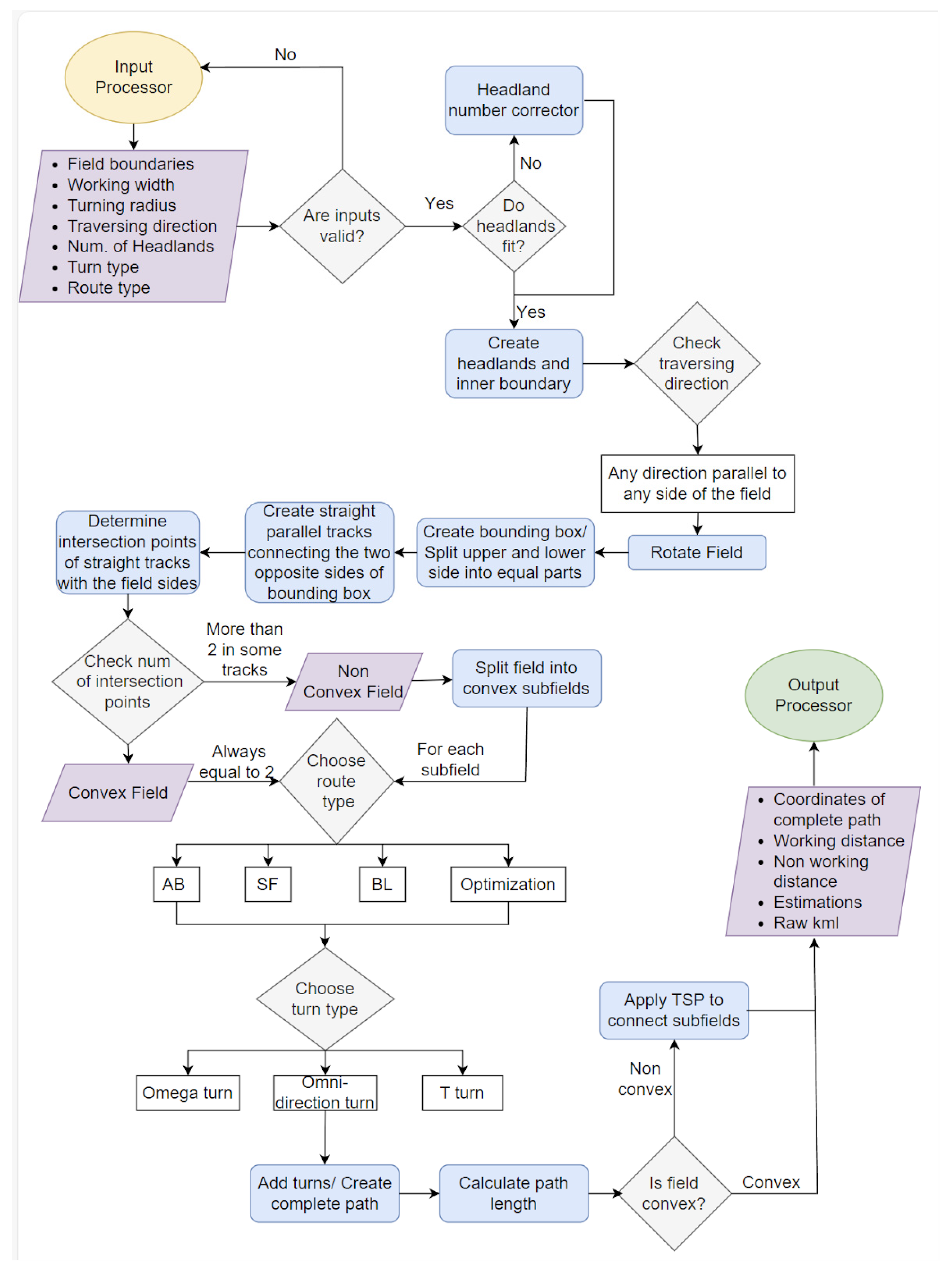
2.2. Route-Planning Module

The first module of the integrated system is the route-planning module. Figure 2 presents the corresponding flow.

2.2.1. Inputs

Six parameters associated with the machinery features are inserted through the FMIS user interface. These parameters are prerequisites for the route-planning module and are described below.

• Working width (w). This refers to the effective operating width and not to the actual width of the carried implement. For example, in a spreading fertilizer application, the effective working width is the range of the fertilizer spread, while, in an orchard, spraying the effective operating width is identical to the inter-row distance.
• UGV’s kinematics. This includes the steering type of the UGV and the corresponding minimum turning radius (r). This variable depends on the type of machinery and, more specifically, on their size and maneuverability, but also on the user preferences in terms of agronomic restrictions. For example, although a UGV can operate under a differential steering system it might be preferable in terms of soil disturbance to follow a smoother turn (r ≠ 0) in order not to disturb the topsoil of the field.
• Traversing direction. For simplicity, the user can select the direction of one of the field vertices as the traversing direction.
• Number of headlands passes. Field area is usually divided into two parts, the headland area, and the field body area. Headland passes describe the concentric paths that the vehicle traverses while in the headland area. These paths consist of sequentially clockwise ordered points. However, as explained later, this user preference can be altered from the system based on the kinematic restrictions of the UGV (for example, to ensure sufficient area for the headland turnings) or based on the field shape complexity (for example, to provide headland passes that do not intersect each other due to sharp field boundary corners).
• Turning type. There are two options: the forward-turn (Ω_turn) and the reverse-turn (T_turn) [41]. The omni-direction turn can be considered a marginal case (where r = 0) in any of these two turning types.
• Route type. Route types can be either predetermined patterns of tracks’ traversal sequence (AB, SF, and BL, as explained in the following), or optimized field-work patterns.

2.2.2. Headland Passes

The number of headland passes is defined by the user. However, there are cases where that number could be reduced or increased by the system. When there is a narrow area in the field or field boundary corners are sharp, headland passes may intersect or overlap [42]. In this case, the number of headland passes set by the user is automatically and gradually reduced by one. Figure 3a illustrates an example where six passes were selected as an input, but they were decreased to four to provide a feasible plan. On the other hand, in cases where the UGV presents a low degree of maneuverability (or agronomic factors impose smooth turnings), the number of headland passes can be increased to ensure that the UGV remains within the boundaries of the field during turns. Figure 3b shows an example where two headland passes were selected by the user; however, four headland passes were created to prevent the UGV from moving outside the field.

The first headland pass was created inside the field at $\raisebox{1ex}{$w$}\!\left/ \!\raisebox{-1ex}{$2$}\right.$ distance from the field boundary. Each subsequent headland pass was at a distance equal to $w$ from the previous one. An inner boundary was created between the headland area and field body area, at half the working width ($\raisebox{1ex}{$w$}\!\left/ \!\raisebox{-1ex}{$2$}\right.$) of the last headland pass.

2.2.3. Route Types

The system provides two classes of route types, namely predefined standard motifs (fieldwork patterns) and optimized routes, in terms of track sequence.

In field operations, field area coverage planning refers to the generation of a set of parallel fieldwork tracks in a distance equal to the machine operating width and the generation of a sequence of traversing these tracks. Based on the model developed in [41], the field area coverage is expressed by the permutation $\sigma =〈p^{-1}\left(1\right), { p}^{-1}\left(2\right), \dots .,{ p}^{-1}\left(\left|T\right|\right)〉$, where $T=\left\{\mathrm{1,2},3,\dots \right\}$ is an arbitrary set of the fieldwork tracks completely covering the field area under a specific operating width, and $p^{-1}\left(·\right):T\to T$ is the inverse function of the bijective function $p\left(·\right):T\to T$ which determines the order in which a machine traverses each fieldwork track.

Regarding the standard fieldwork patterns, the three most common ones were selected for inclusion in the system, namely the AB pattern, the SF patterns (also known as “skip-and-fill”), and the BL pattern (also known as “first-turn-skip”).

The first one, i.e., the AB pattern, is the simplest fieldwork pattern, where the agricultural machine, after covering a fieldwork track, enters the adjacent one. Consequently, $p^{-1}\left(·\right)$ is an identity where $p^{-1}\left(i\right)=i, \forall i\in T$, or $\sigma =〈\mathrm{1,2},3,\dots 〉$ (Figure 4a).

In the SF pattern, the core part of the pattern is a repetition of a standard motif of three tracks, where the track sequence is given by $\sigma =〈\mathrm{1,3},\mathrm{2,5},\mathrm{4,7},\mathrm{6,9},\dots 〉$, (Figure 4b) and the function that describes the motif of the pattern is given by the following equation [43]:

$$p^{-1}\left(i\right)=\left\{\begin{array}{ll}1& i=1\\ 3& i=2\\ p^{-1}\left(i-1\right)& i mod 2=0\\ p^{-1}\left(i-1\right)-1& i mod 2\ne 0\\ \left|T\right|& i=\left|{\rm T}\right| and Tmod3\ne 0\end{array}\right.$$

(1)

Finally, in the BL pattern, the core part of the patterns is a repetition of three tracks that provides the sense of a moving block under the sequence of $\sigma =〈\mathrm{1,3},\mathrm{2,4},\mathrm{6,5},\dots 〉$ (Figure 4c) based on the following motif:

$$p^{-1}\left(i\right)=\left\{\begin{array}{ll}i-1+(i mod 3)& i\ne \left|T\right| or \left|T\right|mod3\ne 2\\ \left|T\right|& i=\left|T\right| and \left|T\right|mod3=2\end{array}\right.$$

(2)

Optimized patterns (B patterns), on the other hand, are algorithmically calculated sequencies of fieldwork tracks based on an optimization process under certain criteria [44]. The case of B patterns was implemented in the present work, a type of optimal field-work pattern produced by the implementation of various vehicle routing problem (VRP) instances, first presented in [41] and implemented in various works on agricultural route-planning [45,46,47,48,49]. B patterns are generated based on the criterion of minimizing the non-working distance travelled by the machine during the field area coverage operation (Figure 4d).

For any traversal sequence, the total non-working distance traveled by an agricultural machine is given by the following equation:

$$J(\sigma )=\sum _{i=1}^{\left|T\right|-1}[c_{0p^{-1}\left(1\right)}+c_{p^{-1}\left(i+1\right),p^{-1}\left(i\right)}+c_{p^{-1}\left|T\right|,\left(f\right)}]$$

(3)

where $c_{0p^{-1}\left(1\right)}$ is the cost of moving from the field entry point to the first track, $c_{p^{-1}\left(i+1\right),{ p}^{-1}\left(i\right)}$ is the cost of moving between two subsequent tracks $p^{-1}\left(i+1\right)$, ${ p}^{-1}\left(i\right)$, and $c_{p^{-1}\left|T\right|,\left(f\right)}$ is the cost of moving from the end of the last covered track to the field exit point. Consequently, the optimization problem consists of finding the optimal permutation, ${\sigma }^{*}=\underset{\sigma }{\mathrm{argmin}}\left[J\left(\sigma \right)\right]$, that minimizes the total non-working distance. For the solution of the specific optimization problem, the field coverage is expressed as the traversal of a weighted graph, where the problem is transformed to find the shortest tour in the weighted graph. This problem can be solved using various approaches to the well-known travelling salesman problem (TSP). In the presented work, a combination of two heuristic algorithms were implemented, namely a greedy-based algorithm and a Clarke–Wright savings algorithm. Figure 4 illustrates the four different patterns provided by the system.

2.2.4. Turn Types

Three different turn types have been defined in the system, namely ${\Omega }_{turn}$, $T_{turn}$, and omni-direction turn. ${\Omega }_{turn}$, also known as Dubins turn, defines the shortest curve from an initial point A to a final point B given the constraint of the minimum turn radius and the fact that the vehicle can only travel forward. $T_{turn}$, on the other hand, provides the shortest curve in cases where the robot can execute both forward and backwards movements. Finally, the omni-direction turn can be considered as a marginal case of the abovementioned two turning types when setting the UGV’s minimum turning radius equal to 0. Figure 5 represents UGV performing the three different turn types in a simulation. Sometimes the entry and exit points of the turn are far apart. In these cases, in a $T_{turn}$, the robot would traverse a prolonged distance backwards. This is not an efficient movement and, for that reason, the route-planning algorithm can replace $T_{turn}$ with an ${\Omega }_{turn}$ for that specific case. The marginal case of the omni-direction turn is depicted in Figure 5c.

2.2.5. Complete Path Generation

In this step, the complete path is produced as an array of coordinates where field-work tracks, turnings, and headland passes are combined. In the case of non-convex-shaped fields, a greedy algorithm is applied to calculate the optimal order to traverse the sub-fields to cover the minimum possible distance.

2.3. FMIS–UGV Communication

For the transmission of the generated path to the CCU, a dedicated endpoint to a Django database was created. An ROS node was developed within the CCU that requires a server’s response to enable the ROS service that was responsible for initiating the operation. The data that were transmitted to the UGV via an API calls consist of an array that includes the coordinates of all points of the path (latitude, longitude), a string that determines if the point belongs to straight path or to the turn path (“track” or “turn”), and a number equal to zero (0) in cases where the vehicle is moving straight forward or to one (1) if the vehicle is moving backwards. The above-mentioned data were transmitted with a JSON data format.

Once communication is established, the UGV begins to receive data from the FMIS. The communication between the FMIS and the CCU took place via the Rest API technology. A dedicated node was developed within the CCU, utilizing ROS and Python to establish communication with the server using the ‘request’ Python library. Once the data are successfully received, the node proceeds to transform the received data into a custom ROS message. Subsequently, it transmits this data to the ROS framework through a navigation stack message. This seamless integration enables effective communication between the UGV and the server. In the specific use-case that is presented in this article, the data are related to GPS coordinates that correspond to the path generated by the system. These data are used by the UGV’s algorithm to generate an automated path for the UGV to follow. This process enables the UGV to navigate autonomously and carry out assigned tasks in an efficient and accurate manner. Additionally, this communication allows for continuous monitoring of the UGV’s progress and condition, enabling timely intervention and adjustments as necessary.

2.4. Data Conversion

To enable FMIS–UGV communication, an intermediate ROS package was required to convert the exchanged data between the two sub-systems. This intermediate package enables the connection of different systems that process varying message formats for the execution of tasks. Furthermore, the message conversion node facilitates interconnection with other FMIS that may use dissimilar formats to transmit data. With minor modifications to the message conversion process between the sub-systems in the data conversion node, it is possible to establish communication without requiring significant changes to the fundamental functions of the communicating systems. This approach simplifies communication and facilitates integration between different systems, enhancing overall efficiency and productivity.

In this scenario, the path data received by the FMIS were transmitted to a JSON-type file. The data-conversion node is responsible for converting these data into a message type that can be managed by ROS. To achieve this, a new message type was developed in ROS that includes the location information of each point on the path in latitude and longitude coordinates, as well as details about the type and direction of movement. The message format is as follows:

$${Msg}_{FMIS}=[{latidude}_{float}; {longitude}_{float}; {routeType}_{std\colon\colon string};{ direction}_{\begin{array}{c}string\\ \end{array}}].$$

The created message contains the endpoints of the path in the form of an array with the information that was mentioned earlier. This information is transmitted by an ROS topic so that it can be retrieved from any ROS node during UGV operation. Before enabling the navigation operation, the generated path should be divided into sub-paths within the local costmap of the UGV that was generated by the Navigation Stack to achieve greater accuracy during the navigation.

The split path is then assigned to a nav_msg/Path-type ROS topic to be compatible with the data types managed by the Navigation Stack.

2.5. Global Frame Creator

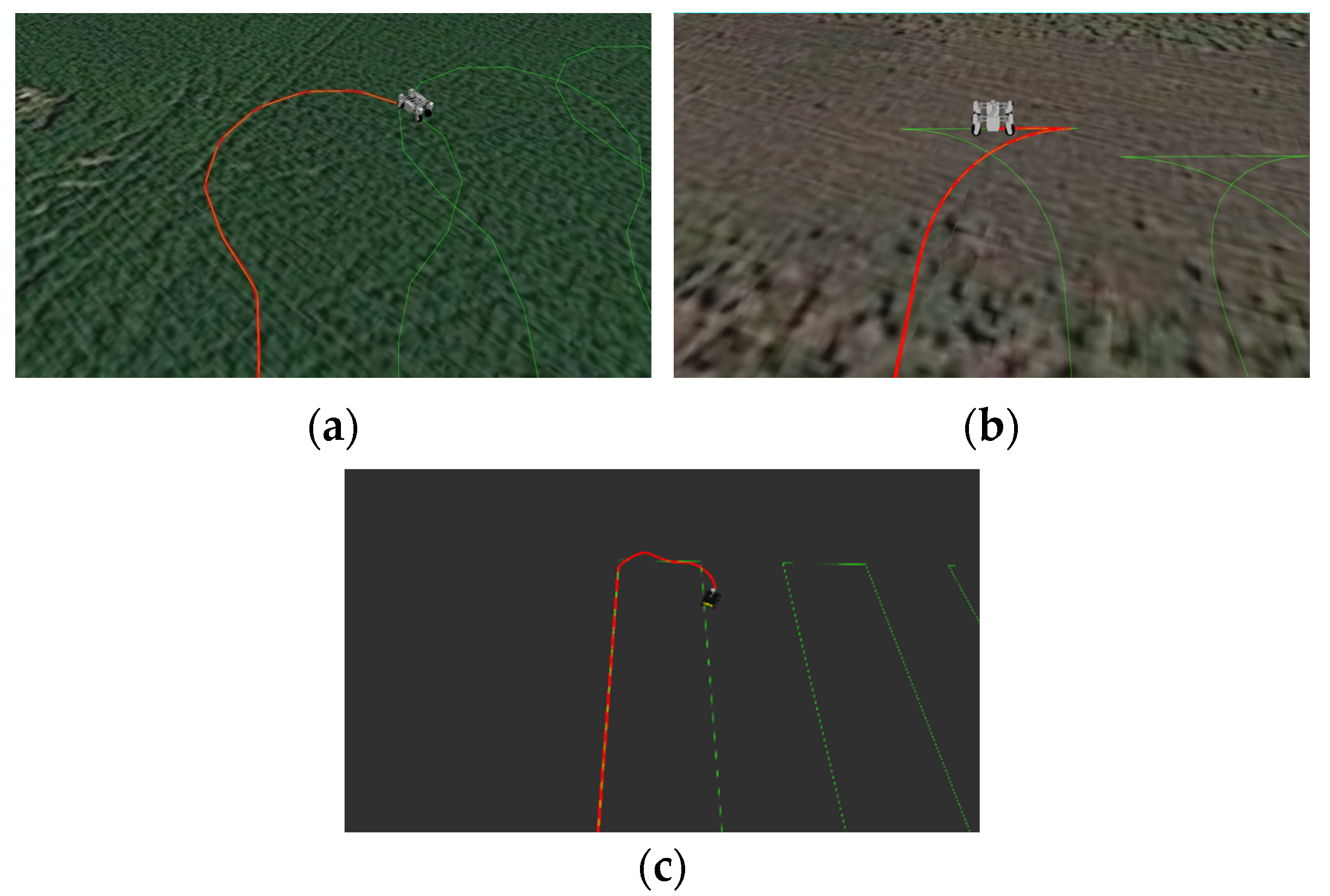
To enable GPS-based navigation, a new frame to the UGV’s TF tree was established that corresponds to the global coordinate system translated into UTM coordinates [50,51,52]. The UGV is positioned within this frame and updates its location within the global frame based on data received from the GPS sensor that was mounted on the UGV. The global frame was created using a TF broadcaster from the TF ROS library [53], which allowed for the definition of a new frame and the movement of the existing TF tree (Odom–UGV). The displacement being referred to was the result of the latitude and longitude positions obtained from the GPS sensor, which are then translated into UTM coordinates.

2.6. UGV Navigation

To enable the navigation of the UGV and execute the mission received from the FMIS, modifications were made to the Navigation Stack. The changes primarily involved the ROS NavFN Global Planner. To accomplish this, a library was created and added to the ROS Navfn package. Its purpose was to obtain the ROS topic that contains the split path and assign it to the node of Navfn. Additionally, this library could correct any deviation from the desired path due to UGV sliding. This correction occurs during the transformation of each path point from the Global frame to the Odom frame in which the navigation takes place. Testing has shown that assigning the path to the global planner does not affect the other functions of the Navigation Stack, such as obstacle avoidance, as this function is based on a local planner [52,54,55].

2.7. Analytics Module

The CCU provides data about the total traversing distance, total time, and average speed of the UGV while following the complete path. This information is directed to a module that calculates analytics concerning UGV’s movement in the field. In this module, analytics from simulations were also computed for comparison with analytics from the UGV’s movement.

The performance indicators include the working distance, non-working distance, overlapped area, and field-traversing efficiency (FTE) [56]. Working distance represents the productive (effective) distance that the UGV traverses to complete the operation. It includes the length of headland passes and fieldwork tracks. Non-working distance describes the non-productive driving distance while the UGV performs turns or moves from one sub-field to another via headlands in the case of non-convex-shaped fields. The overlapped area is equal to the difference between the covered area and the total field area. Finally, the field-traversal efficiency (FTE) index is calculated as a distance-based measure to evaluate the productivity of the routing plan [57]. FTE is a distance-based evaluation that takes into consideration unique features of the field, namely its shape and area, as well as machinery specifications like operating width and turning radius. Furthermore, other operational aspects, such as driving direction and fieldwork patterns, are also an essential part of the FTE. The mathematical formula of FTE is given below [57,58]:

$$FTE=\frac{{\sum }_{i=1}^{h}d\left(H_i\right)+{\sum }_{i=1}^{n}d\left(T_i\right)}{d\left(p\right)}$$

(4)

where ${\sum }_{i=1}^{h}d\left(H_i\right)$ is the total length of all headland passes, ${\sum }_{i=1}^{n}d\left(T_i\right)$ is the total length of tracks, and $d\left(p\right)$ is the total length of the path, including the length of turns and length of the distance from one sub-field to another.

3. System Demonstration

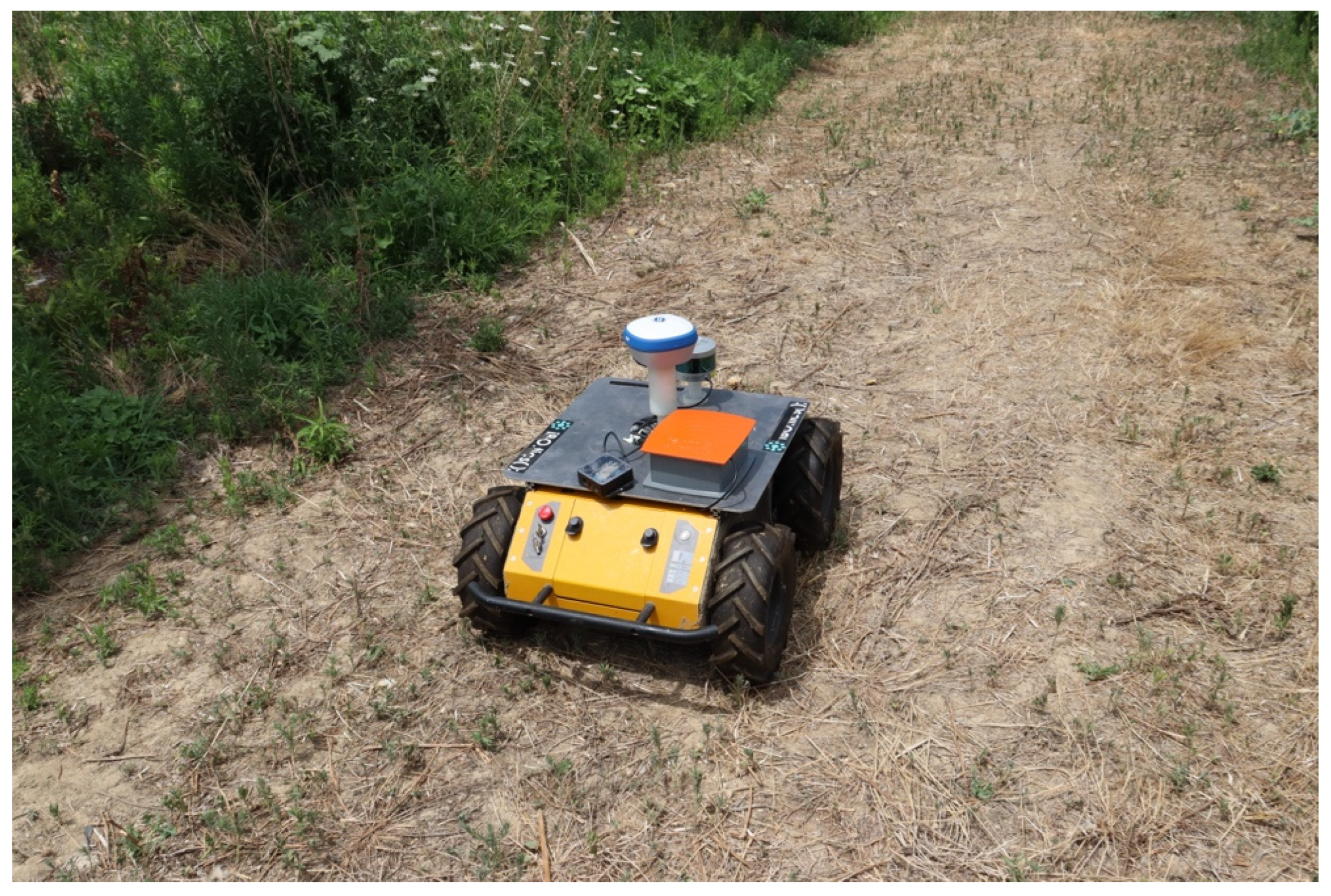
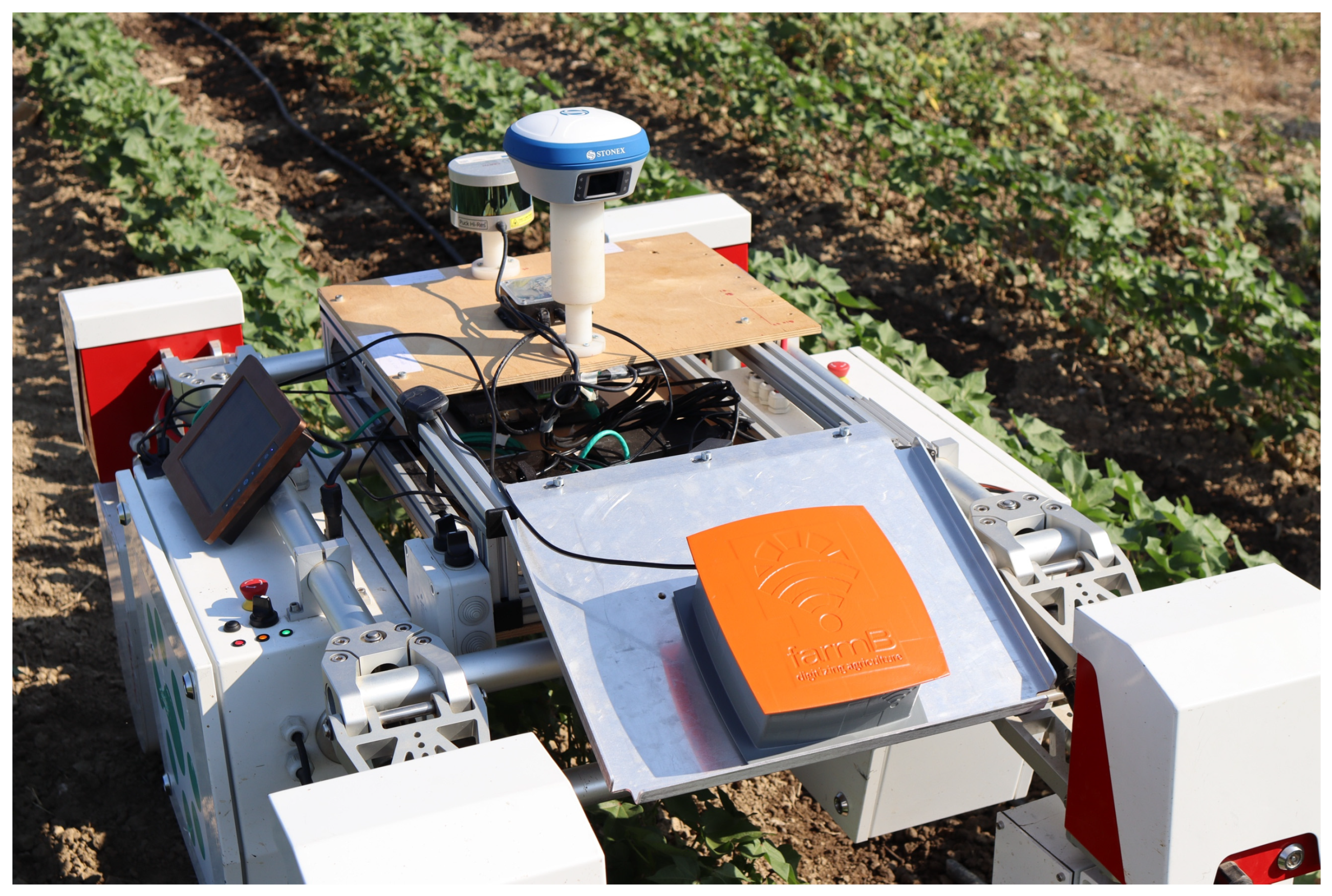
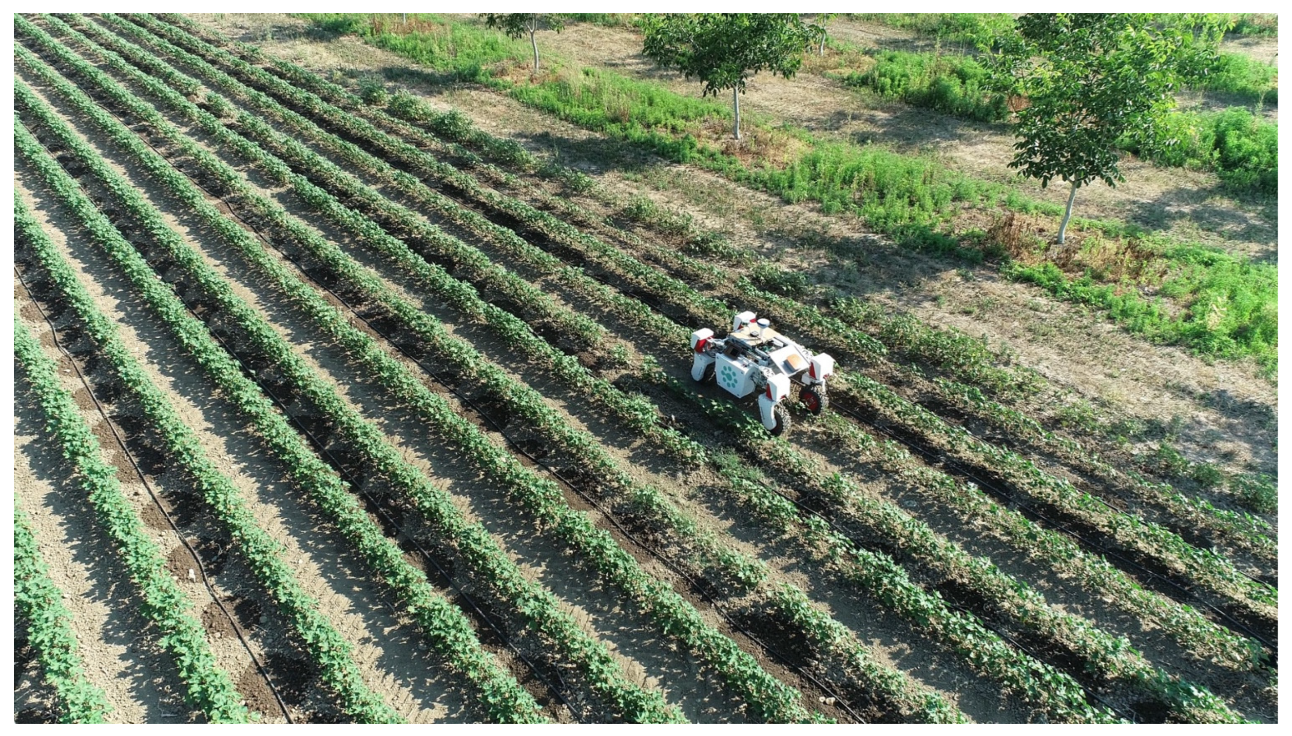
3.1. Mobile Platforms

For the system demonstration, two UGVs were implemented. The first one was Husky (Clearpath Robotics Inc.: Kitchener, Canada), which uses differential steering, as shown in Figure 6. The second one was a four-wheel drive (4WD), four-wheel steering (4WS) UGV, Thorvald (Saga Robotics, Oslo, Norway (Figure 7). This UGV, after specific programming interventions, can alternate its movement between four-wheel, holonomic, and Ackermann steering. Both UGVs can navigate autonomously and follow the generated route while avoiding both dynamic and static obstacles.

A set of various sensors were embedded to the UGVs to ensure the proper and safe execution of the generated paths. A lidar sensor (specifically, the Velodyne VLP 16) was utilized to scan and map the surrounding area [59,60]. This sensor allowed for the creation of a two-dimensional dynamic map that identifies and marks any obstacles that are present [61]. To ensure accurate positioning, a GNSS-RTK receiver (STONEX S990A RTK) was incorporated into the UGVs. The GNSS-RTK receiver provides precise latitude and longitude coordinates to the navigation system, enabling the UGV to accurately determine its location within the field. This specific RTK receiver, when connected to a base station, is capable of achieving a 5 mm + 0.5 ppm RMS fixed and 10 mm + 0.5 ppm RMS accuracy for a fixed RTK horizontal and vertical position, respectively, with the position rate of 10 Hz. In the cases that are examined in the current study, the receiver was connected to a nearby base station via an end-trip server to reach the above-mentioned maximum accuracy. In addition to the above, an IMU (UM7) sensor was incorporated, along with the implementation of the Kalman Filter, to assist in the automated navigation. The UM7 orientation sensor, developed by Redshift Labs, stands as a third-generation Attitude and Heading Reference System (AHRS). It efficiently generates attitude and heading estimates by processing triaxial accelerometer, rate gyro, and magnetometer data, with sensor specifications of ±2000° s⁻¹ (gyro), ±8 g (accelerometer), and ±12 gauss (magnetometer). Unlike a standard inertial measurement unit (IMU), which provides raw sensor readings, the UM7 is equipped with an onboard microcontroller. This microcontroller employs an Extended Kalman Filter (EKF) to integrate sensor data, enabling the generation of orientation estimates at a rate of 500 t s¹. Finally, the CCU (developed by farmB digital agriculture S.A.: Thessaloniki, Greece) of the system was mounted to enable real-time, two-way communication between the FMIS (farmB digital agriculture S.A., Greece) and the UGVs. Furthermore, the CCU was responsible (i) for providing the UGV with all the necessary data for the execution of the generated path and (ii) for generating and transmitting the records of the executed operation. The abovementioned CCU was powered by an AGX Orin system-on-module (SoM) developed by NVIDIA.

Two different UGVs were selected for the pilot testing of this current research. These UGVs differ not only based on their size but also in terms of their physical properties. The first UGV (Thorvald) has wheels that can be rotated along their vertical axes providing the ability to navigate either under holonomic (e.g., omnidirectional steering) or non-holonomic (e.g., Ackerman steering) conditions. For the purpose of this research, the type of steering that was used in the pilot implementations was the latter one, as a way to demonstrate the feasibility of implementing the proposed system in conventional tractors or tractor-like field robots. The second UGV (Husky) has two (2) motors and turns under differential steering. The selection of two different types of UGVs was chosen so the developed algorithms could properly demonstrate their applicability to different UGV types and steering mechanisms.

3.2. Case Studies

The first set of experiments regarded various pilots of the system in two experimental fields cultivated with wheat, one of a convex shape and area of 2.54 ha (field A), and one of a non-convex shape and area of 6.81 ha (field B), both located in Thessaly, Greece. The scope of these runs was as follows:

• To show the ability of the system to generate various configurations of plans as functions of different fieldwork patterns, operating directions, vehicle turning radius, and operating widths;
• To show the differentiation in operating efficiency (FTE) for different configurations;
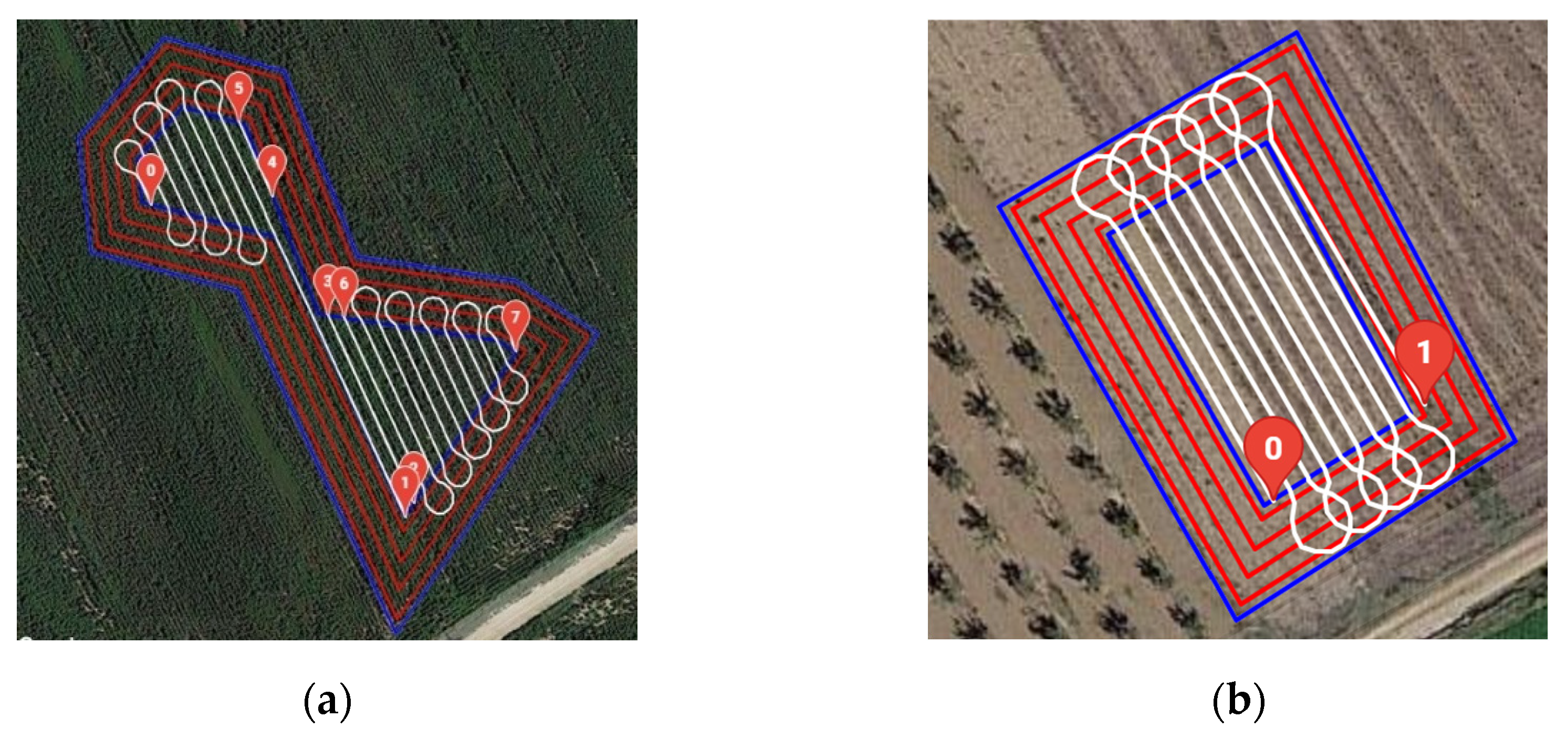
• To show the ability of the system to provide feasible plans for both convex and non-convex field shapes.

In total, 36 runs were performed for each of the two fields. These 36 runs are the results of the selected combination of three working widths (1.5 m, 3 m, and 4.5 m), two values of the UGV minimum turning radius (3 m and 6 m), three types of fieldwork patterns (AB, SF, and BL), and two driving directions (longest edge of the field—DIR_1—and its perpendicular or the area closer to this field edge—DIR_2). The average speed of the UGV (Thorvald) during the operation was set to 2 m s⁻¹ in straight paths and 0.5 m s⁻¹ in turning paths.

Examples of the cases that were run are presented in Figure 8, where the generated and actual executed paths are presented under the following configurations:

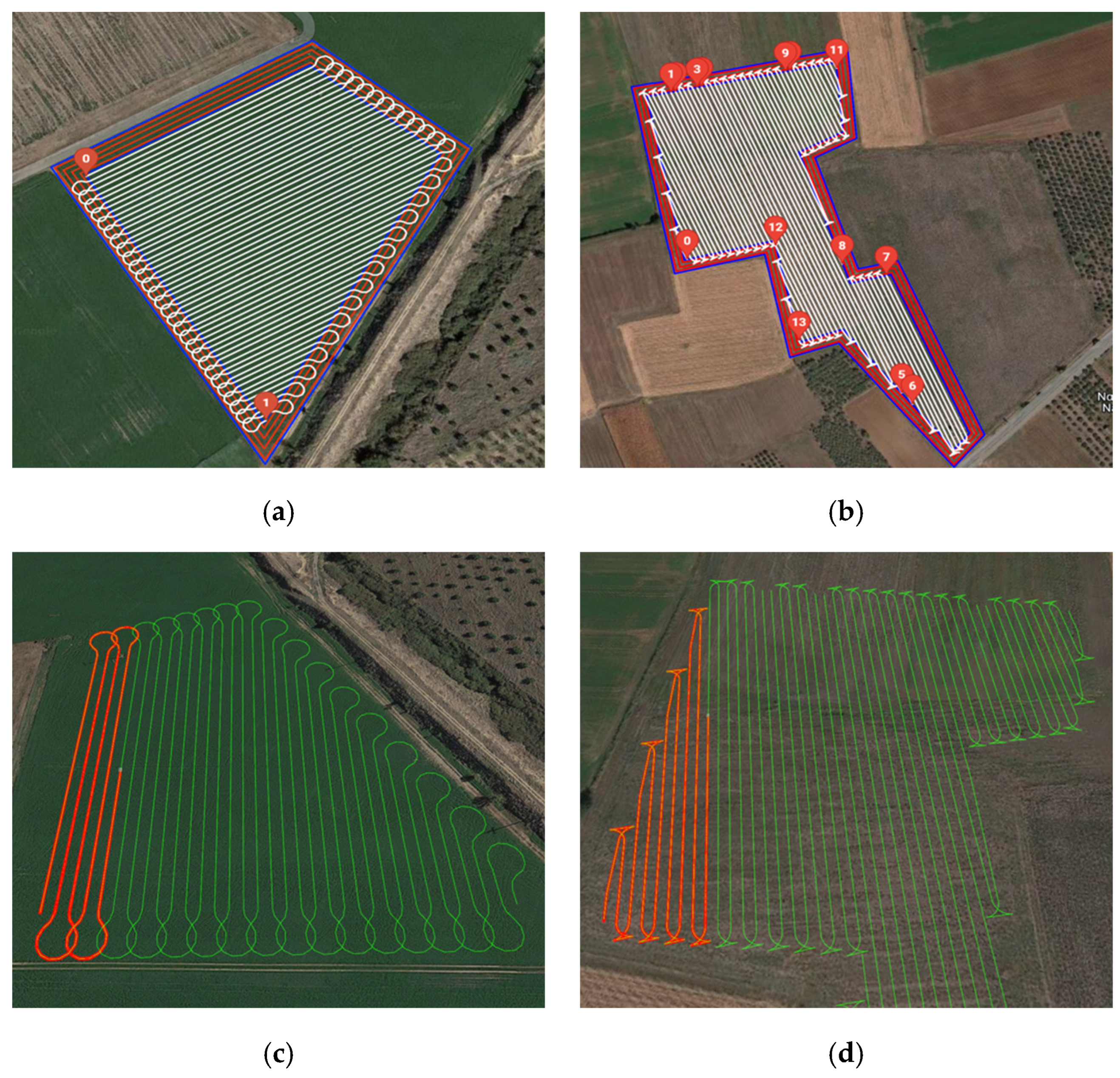
• Field A (under grass cultivation): w = 4.5 m, r = 6 m, turn type → Ω_turn, and driving direction parallel to the longest edge of the field (Figure 8a,c);
• Field B (under wheat cultivation), w = 4.5 m, r = 6 m, turn type → T_turn, and driving direction parallel to the longest edge of the field (Figure 8b,d).

The evaluation of the 36 different use-cases involved the utilization of the FTE index. A visualization of the results of all use-cases in terms of FTE performance is provided in Figure 9 and Figure 10. The first chart (Figure 9) illustrates the results for Field A. The highest value of FTE (0.93) was observed when the UGV performs the AB route type operating parallel to the longest edge of the field (DIR_1), with an operating width of 4.5 m and a minimum turning radius of 3 m. Conversely, the lowest value of FTE (0.797) was observed in the use-case of the AB route type, where UGV was operating parallel to direction DIR_2, with an operating width of 1.5 m and minimum turning radius of 6 m. The average FTE index value for all the use cases for field A was 0.873.

The second chart (Figure 10) presents the FTE index outcomes for Field B. The maximum and minimum FTE occur in the same use-cases as in Field A. More specifically, the maximum value of FTE was 0.922, while the minimum was found to be 0.792. Across all use-cases in field B, the average FTE was 0.874.

A second set of experiments regarded the planning and execution of optimal area coverage plans. Two configurations were selected for the same experimental fields for the comparison between the optimal plans and the standard fieldwork patterns’ motifs, as follows:

• Configuration 1: w = 1.5 m, r = 6 m, and direction ≡ DIR_1.
• Configuration 2: w = 4.5 m, r = 3 m, and direction ≡ DIR_2.

The logic behind the selection of the two specific configuration is to show the benefits of having optimal plans at two opposite edges, namely, a “soft” configuration (configuration 2), in terms of non-working distance (minimum turning radius shorter than working width and a low number of headland turns), where the benefits derived from the implementation of the optimal path are expected to be of a low level, and a “hard” configuration (configuration 1) in terms of non-working distance (minimum turning radius longer than working width and a high number of headland turns), where the benefits derived from the implementation of optimal paths are expected to be of a high level.

For the operations executed under configuration 1,

Table 1. Configuration 1 for the case of field A.

	Total Distance (m)	Non-Working Distance (m)	Savings (%)	FTE (%)	FTE Improvement (%)
OPT	16,867.67	2211.76	_	88.4	_
AB	21,151.77	4284.1	48.37	79.7	8.7
SF	20,705.95	3838.28	42.38	81.5	6.9
BL	20,708.68	3841.01	42.4	81.5	6.9

presents total distance (m), non-working distance (m), savings, FTE, and the improvement in FTE for the case of field A, while

Table 2. Configuration 1 for the case of field B.

	Total Distance (m)	Non-Working Distance (m)	Savings (%)	FTE (%)	FTE Improvement (%)
OPT	50,812.12	5733.75	_	88.7
AB	56,892.59	11,814.22	51.47	79.2	9.5
SF	55,997.98	10,919.61	47.49	80.5	8.2
BL	56,002.98	10,924.38	47.51	80.5	8.2

shows the corresponding results for the case of field B. Analogously, for the operations executed under configuration 2, the corresponding results are presented in

Table 3. Configuration 2 for the case of field A.

	Total Distance (m)	Non-Working Distance (m)	Savings (%)	FTE (%)	FTE Improvement (%)
OPT	6046.38	403.27	_	93.3	_
AB	6069.94	426.83	5.52	93	0.3
SF	6163.44	520.33	22.5	91.6	1.7
BL	6183.08	539.97	25.32	91.3	2

and

Table 4. Configuration 2 for the case of field B.

	Total Distance (m)	Non-Working Distance (m)	Savings (%)	FTE (%)	FTE Improvement (%)
Opt	16,380.74	1183.98	_	92.8	_
AB	16,492.28	1295.52	8.61	92.2	0.6
SF	16,663.11	1466.35	19.26	91.2	1.6
BL	16,644.86	1448.1	18.24	91.3	1.5

for the cases of field A and field B, respectively.

The term “FTE improvement” refers to the difference in FTE between the optimal path and the conventional paths (AB, SF, and BL). As an example, the value 8.7% in the case of configuration 1—field A—AB pattern means that, for a travelled distance of 100 m, the non-working part, in the case of the optimal route, is reduced by 8.7 m compared to that of the AB pattern. This outperformance of the optimal plans suggests that optimal routes lead to time savings and resource optimization.

The third set of experiments demonstrates the applicability of the developed system in the case of a structured field operating environment, namel, for operation in row crops and in orchard environments. The field configuration (distance between crop rows or between tree rows) is information that exists in the FMIS field database, and the track generation process automatically considers the restrictions on the distance between adjusted tracks [62,63,64].

The first experiment focuses on demonstrating the system’s performance in cotton fields as an example of row crop cultivation (Figure 11). Thorvald robot was employed for that task. The reason that this UGV was chosen is that its structure is better-suitable to navigating over the rows without causing damage to the crop. In the selected field, cotton rows were arranged in an inter-row distance of 0.9 m. Three distinct scenarios were generated and run, each corresponding to different working widths of 0.9 m, 2.7 m, and 5.4 m, as illustrated in Figure 12a–c, respectively.

In the case of orchard operations, the structure of the orchard field is stored in the FMIS database, and the system can provide routes for operations that are performed in the middle of the row (e.g., spraying operations) or operations where passes are focused on one side of the tree row (e.g., monitoring operation) at a pre-defined distance. The experiments were conducted in a walnut tree orchard, where inter-row distance is equal to 8 m. Husky UGV was used for this experiment (Figure 13). In the first use-case, tracks were set at a fixed distance of 4 m from each tree row (Figure 14a). Husky was used to test the route-planning module on a different robotic platform. In the second use-case, designed for tasks requiring dedicated passes along one side of the tree row, two separated tracks were formed within each inter-row space (Figure 14b). More specifically, the first track was 2 m from the first orchard row, while the second track was created 6 m from it (or, equivalently, 2 m distance for the one adjacent to the first track). This configuration facilitates precise navigation for tasks that require targeted passes along the side of the tree row. In both use-cases, an omni-direction turn type was followed.

4. Discussion and Conclusions

Τhis paper presented the basis for an integrated system for agri-robotics, enabling two-way communication between an unmanned ground vehicle (UGV) and a farm management information system (FMIS) under the general scope of smart farming implementation. In this initial step, the primary task of route-planning for agricultural vehicles, as a prerequisite for the execution of any field operation, was selected as a use-case for building and evaluating this integration.

The representation of results in the user interface provides the opportunity for the user to better control their farm–field operations and to make alterations to ensure optimal route-planning. The successful autonomous navigation of an agricultural robot in real-word conditions based on plans created by the route-planning module indicates the effectiveness and applicability of the proposed system. The system can handle cases involving convex and non-convex field shapes and can be adapted to different turn types, fieldwork patterns, including optimized ones, working widths, and vehicle kinematics. The system is applicable in various row-based crops when aiming to cover parallel fieldwork tracks. This includes, in principle, all arable farming operations, including full field-area crop coverage (e.g., wheat) and row crops (e.g., cotton), where the vehicle wheels should only be placed in uncultivated strips, as well as orchard operations where inter-row strips are parallel and a headland area is available for the vehicle turnings. The flexibility provided to the user in selecting different operational features can lead to the creation of the most efficient path based on field geometry and the UGV’s kinematics. The case studies showed variability in the operational performance to allow for the field traversal efficiency to be between 79.2% and 93%, while, when implementing the optimal route-planning functionality of the system, there was an improvement of up to 9.5% in the field efficiency. By considering operational factors, the non-working distance can be effectively minimized, and the operation execution time can be reduced, leading to a decrease in operational costs. The user interface provides an interactive tool for the before-operation simulation and testing to allow for the selection of the most efficient field coverage configuration. For example, Figure 15 shows the results of a use-case in the first experiment as presented to the user interface. On the left side, all users’ input parameters are displayed. In the center of the interface, a dynamic map visualization is illustrated, which depicts the route that was created over the field to allow for a better spatial understanding. On the right side, an estimation of total working distance, non-working distance, headland distance, field body distance, overlapped area, and field efficiency are displayed. The “send navigation plan” button allows for the direct transfer of the generated navigation plan to the “connected” UGV.

The system utilizes the ROS, ensuring data exchange without requiring significant changes to the fundamental functions of the communicating systems. Substantial advancements have been achieved through the addition of new frames to the UGV’s TF tree, corresponding to the global coordinate system translated into UTM coordinates. This adaptation enhances the system’s applicability to real-world conditions. Modifications to the ROS navigation stack, specifically the NavFN global planner, improve the UGV’s navigation efficiency by addressing deviations and refining path tracking.

The central part of the system is the developed communicational and computational unit (CCU) that facilitates real-time, two-way communication between the FMIS and UGV and ensures that all necessary data are effectively transferred from one to another. As previously shown, the CCU is completely adaptable between the two different UGVs that were implemented for the demonstration of the system, and, in principle, can be adapted to any other ROS-enabled robotic system. Furthermore, the CCU was built under a scalability model to allow new functions to be added. These functions, as a matter of future research and development, include the following:

• The recording and transition of operational data, e.g., crop health monitoring data, to the FMIS;
• The recording and transition UGV performance data, e.g., power consumption and task times;
• The transition to the UGV of complete mission-planning data, for example, variable rate application plans and task schedules, combined with route plans;
• The inclusion of AI capabilities for human–UGV interaction processes.

Furthermore, the feedback loop between the UGV and the FMIS will allow for FMIS to have self-learning capabilities that can provide more customized solutions for specific fields and conditions.

References

1. Lytos, A.; Lagkas, T.; Sarigiannidis, P.; Zervakis, M.; Livanos, G. Towards smart farming: Systems, frameworks and exploitation of multiple sources. Comput. Netw. 2020, 172, 107147. [Google Scholar] [CrossRef]
2. Yadav, S.; Kaushik, A.; Sharma, M.; Sharma, S. Disruptive Technologies in Smart Farming: An Expanded View with Sentiment Analysis. AgriEngineering 2022, 4, 424–460. [Google Scholar] [CrossRef]
3. Žuraulis, V.; Pečeliūnas, R. The Architecture of an Agricultural Data Aggregation and Conversion Model for Smart Farming. Appl. Sci. 2023, 13, 11216. [Google Scholar] [CrossRef]
4. Sharma, V.; Tripathi, A.K.; Mittal, H. Technological revolutions in smart farming: Current trends, challenges & future directions. Comput. Electron. Agric. 2022, 201, 107217. [Google Scholar] [CrossRef]
5. Gao, Z.; Luo, Z.; Zhang, W.; Lv, Z.; Xu, Y. Deep Learning Application in Plant Stress Imaging: A Review. AgriEngineering 2020, 2, 430–446. [Google Scholar] [CrossRef]
6. Hardy, T.; Kooistra, L.; Franceschini, M.D.; Richter, S.; Vonk, E.; van den Eertwegh, G.; van Deijl, D. Sen2Grass: A Cloud-Based Solution to Generate Field-Specific Grassland Information Derived from Sentinel-2 Imagery. AgriEngineering 2021, 3, 118–137. [Google Scholar] [CrossRef]
7. Chowdhury, M.E.H.; Rahman, T.; Khandakar, A.; Ayari, M.A.; Khan, A.U.; Khan, M.S.; Al-Emadi, N.; Reaz, M.B.I.; Islam, M.T.; Ali, S.H.M. Automatic and Reliable Leaf Disease Detection Using Deep Learning Techniques. AgriEngineering 2021, 3, 294–312. [Google Scholar] [CrossRef]
8. Doshi, J.; Patel, T.; kumar Bharti, S. Smart Farming using IoT, a solution for optimally monitoring farming conditions. Procedia Comput. Sci. 2019, 160, 746–751. [Google Scholar] [CrossRef]
9. Sirimorok, N.; Paweroi, R.M.; Arsyad, A.A.; Köppen, M. Smart Farm Security by Combining IoT Sensor Network and Virtualized Mycelium Network. Sensors 2023, 23, 8689. [Google Scholar] [CrossRef]
10. Bhat, S.A.; Huang, N.F.; Sofi, I.B.; Sultan, M. Agriculture-Food Supply Chain Management Based on Blockchain and IoT: A Narrative on Enterprise Blockchain Interoperability. Agriculture 2021, 12, 40. [Google Scholar] [CrossRef]
11. Lioutas, E.D.; Charatsari, C. Smart farming and short food supply chains: Are they compatible? Land Use Policy 2020, 94, 104541. [Google Scholar] [CrossRef]
12. Aliyu, A.A.; Liu, J.; Aliyu, A.A.; Liu, J. Blockchain-Based Smart Farm Security Framework for the Internet of Things. Sensors 2023, 23, 7992. [Google Scholar] [CrossRef]
13. Jararweh, Y.; Fatima, S.; Jarrah, M.; AlZu’bi, S. Smart and sustainable agriculture: Fundamentals, enabling technologies, and future directions. Comput. Electr. Eng. 2023, 110, 108799. [Google Scholar] [CrossRef]
14. Dhanaraju, M.; Chenniappan, P.; Ramalingam, K.; Pazhanivelan, S.; Kaliaperumal, R. Smart Farming: Internet of Things (IoT)-Based Sustainable Agriculture. Agriculture 2022, 12, 1745. [Google Scholar] [CrossRef]
15. Hazim, Z.; Azlan, Z.; Junaini, N.; Alamshah Bolhassan, N.; Wahi, R.; Arip, M.A. Harvesting a sustainable future: An overview of smart agriculture’s role in social, economic, and environmental sustainability. J. Clean. Prod. 2024, 434, 140338. [Google Scholar] [CrossRef]
16. Daum, T.; Baudron, F.; Birner, R.; Qaim, M.; Grass, I. Addressing agricultural labour issues is key to biodiversity-smart farming. Biol. Conserv. 2023, 284, 110165. [Google Scholar] [CrossRef]
17. Chen, H.Y.; Sharma, K.; Sharma, C.; Sharma, S. Integrating explainable artificial intelligence and blockchain to smart agriculture: Research prospects for decision making and improved security. Smart Agric. Technol. 2023, 6, 100350. [Google Scholar] [CrossRef]
18. Rettore de Araujo Zanella, A.; da Silva, E.; Pessoa Albini, L.C. Security challenges to smart agriculture: Current state, key issues, and future directions. Array 2020, 8, 100048. [Google Scholar] [CrossRef]
19. Wiseman, L.; Sanderson, J.; Zhang, A.; Jakku, E. Farmers and their data: An examination of farmers’ reluctance to share their data through the lens of the laws impacting smart farming. NJAS Wagening. J. Life Sci. 2019, 90–91, 100301. [Google Scholar] [CrossRef]
20. van der Burg, S.; Bogaardt, M.J.; Wolfert, S. Ethics of smart farming: Current questions and directions for responsible innovation towards the future. NJAS Wagening. J. Life Sci. 2019, 90–91, 100289. [Google Scholar] [CrossRef]
21. Mark, R. Ethics of Using AI and Big Data in Agriculture: The Case of a Large Agriculture Multinational. ORBIT J. 2019, 2, 1–27. [Google Scholar] [CrossRef]
22. Amiri-Zarandi, M.; Dara, R.A.; Duncan, E.; Fraser, E.D.G. Big Data Privacy in Smart Farming: A Review. Sustainability 2022, 14, 9120. [Google Scholar] [CrossRef]
23. Cordova-Cardenas, R.; Emmi, L.; Gonzalez-de-Santos, P. Enabling Autonomous Navigation on the Farm: A Mission Planner for Agricultural Tasks. Agriculture 2023, 13, 2181. [Google Scholar] [CrossRef]
24. Cantelli, L.; Bonaccorso, F.; Longo, D.; Melita, C.D.; Schillaci, G.; Muscato, G. A Small Versatile Electrical Robot for Autonomous Spraying in Agriculture. AgriEngineering 2019, 1, 391–402. [Google Scholar] [CrossRef]
25. Iberraken, D.; Gaurier, F.; Roux, J.C.; Chaballier, C.; Lenain, R. Autonomous Vineyard Tracking Using a Four-Wheel-Steering Mobile Robot and a 2D LiDAR. AgriEngineering 2022, 4, 826–846. [Google Scholar] [CrossRef]
26. Moysiadis, V.; Tsolakis, N.; Katikaridis, D.; Sørensen, C.G.; Pearson, S.; Bochtis, D. Mobile Robotics in Agricultural Operations: A Narrative Review on Planning Aspects. Appl. Sci. 2020, 10, 3453. [Google Scholar] [CrossRef]
27. Kaleem, A.; Hussain, S.; Aqib, M.; Jehanzeb, M.; Cheema, M.; Saleem, S.R.; Farooq, U.; Pk, M.J.M.C. Development Challenges of Fruit-Harvesting Robotic Arms: A Critical Review. AgriEngineering 2023, 5, 2216–2237. [Google Scholar] [CrossRef]
28. Katikaridis, D.; Moysiadis, V.; Tsolakis, N.; Busato, P.; Kateris, D.; Pearson, S.; Sørensen, C.G.; Bochtis, D. UAV-Supported Route Planning for UGVs in Semi-Deterministic Agricultural Environments. Agronomy 2022, 12, 1937. [Google Scholar] [CrossRef]
29. Moysiadis, V.; Katikaridis, D.; Benos, L.; Busato, P.; Anagnostis, A.; Kateris, D.; Pearson, S.; Bochtis, D. An Integrated Real-Time Hand Gesture Recognition Framework for Human–Robot Interaction in Agriculture. Appl. Sci. 2022, 12, 8160. [Google Scholar] [CrossRef]
30. Bechar, A.; Vigneault, C. Agricultural robots for field operations: Concepts and components. Biosyst. Eng. 2016, 149, 94–111. [Google Scholar] [CrossRef]
31. Lauretti, C.; Tamantini, C.; Tomè, H.; Zollo, L. Robot Learning by Demonstration with Dynamic Parameterization of the Orientation: An Application to Agricultural Activities. Robotics 2023, 12, 166. [Google Scholar] [CrossRef]
32. Bechar, A.; Edan, Y. Human-robot collaboration for improved target recognition of agricultural robots. Ind. Robot 2003, 30, 432–436. [Google Scholar] [CrossRef]
33. Seyyedhasani, H.; Peng, C.; Jang, W.; Vougioukas, S.G. Collaboration of human pickers and crop-transporting robots during harvesting—Part II: Simulator evaluation and robot-scheduling case-study. Comput. Electron. Agric. 2020, 172, 105323. [Google Scholar] [CrossRef]
34. Vasconez, J.P.; Kantor, G.A.; Auat Cheein, F.A. Human–robot interaction in agriculture: A survey and current challenges. Biosyst. Eng. 2019, 179, 35–48. [Google Scholar] [CrossRef]
35. Lytridis, C.; Kaburlasos, V.G.; Pachidis, T.; Manios, M.; Vrochidou, E.; Kalampokas, T.; Chatzistamatis, S. An Overview of Cooperative Robotics in Agriculture. Agronomy 2021, 11, 1818. [Google Scholar] [CrossRef]
36. Adamides, G.; Katsanos, C.; Parmet, Y.; Christou, G.; Xenos, M.; Hadzilacos, T.; Edan, Y. HRI usability evaluation of interaction modes for a teleoperated agricultural robotic sprayer. Appl. Ergon. 2017, 62, 237–246. [Google Scholar] [CrossRef]
37. McCaig, M.; Dara, R.; Rezania, D. Farmer-centric design thinking principles for smart farming technologies. Internet Things 2023, 23, 100898. [Google Scholar] [CrossRef]
38. Wang, T.; Xu, X.; Wang, C.; Li, Z.; Li, D. From Smart Farming towards Unmanned Farms: A New Mode of Agricultural Production. Agriculture 2021, 11, 145. [Google Scholar] [CrossRef]
39. Koubaa, A. Robot Operating System (ROS): The Complete Reference (Volume 1), 1st ed.; Springer International Publishing: Cham, Switzerland, 2016; ISBN 3319260529. [Google Scholar]
40. Megalingam, R.K.; Rajendraprasad, A.; Manoharan, S.K. Comparison of Planned Path and Travelled Path Using ROS Navigation Stack. In Proceedings of the 2020 International Conference for Emerging Technology (INCET), Belgaum, India, 5–7 June 2020; pp. 1–6. [Google Scholar]
41. Bochtis, D.D.; Vougioukas, S.G. Minimising the non-working distance travelled by machines operating in a headland field pattern. Biosyst. Eng. 2008, 101, 1–12. [Google Scholar] [CrossRef]
42. Höffmann, M.; Patel, S.; Büskens, C. Optimal Coverage Path Planning for Agricultural Vehicles with Curvature Constraints. Agriculture 2023, 13, 2112. [Google Scholar] [CrossRef]
43. Bochtis, D.D.; Sørensen, C.G.; Busato, P.; Berruto, R. Benefits from optimal route planning based on B-patterns. Biosyst. Eng. 2013, 115, 389–395. [Google Scholar] [CrossRef]
44. Bochtis, D.D.; Sørensen, C.G. The vehicle routing problem in field logistics part I. Biosyst. Eng. 2009, 104, 447–457. [Google Scholar] [CrossRef]
45. Utamima, A.; Reiners, T.; Ansaripoor, A.H. Optimisation of agricultural routing planning in field logistics with Evolutionary Hybrid Neighbourhood Search. Biosyst. Eng. 2019, 184, 166–180. [Google Scholar] [CrossRef]
46. Utamima, A.; Reiners, T.; Ansaripoor, A.H. Evolutionary neighborhood discovery algorithm for agricultural routing planning in multiple fields. Ann. Oper. Res. 2022, 316, 955–977. [Google Scholar] [CrossRef]
47. Seyyedhasani, H.; Dvorak, J.S. Reducing field work time using fleet routing optimization. Biosyst. Eng. 2018, 169, 1–10. [Google Scholar] [CrossRef]
48. Conesa-Muñoz, J.; Pajares, G.; Ribeiro, A. Mix-opt: A new route operator for optimal coverage path planning for a fleet in an agricultural environment. Expert Syst. Appl. 2016, 54, 364–378. [Google Scholar] [CrossRef]
49. Jing, Y.; Luo, C.; Liu, G. Multiobjective path optimization for autonomous land levelling operations based on an improved MOEA/D-ACO. Comput. Electron. Agric. 2022, 197, 106995. [Google Scholar] [CrossRef]
50. Guimarães, R.L.; de Oliveira, A.S.; Fabro, J.A.; Becker, T.; Brenner, V.A. ROS Navigation: Concepts and Tutorial. In Robot Operating System (ROS): The Complete Reference (Volume 1); Koubaa, A., Ed.; Springer International Publishing: Cham, Switzerland, 2016; pp. 121–160. ISBN 978-3-319-26054-9. [Google Scholar]
51. Vieira, D.; Orjuela, R.; Spisser, M.; Basset, M. Positioning and Attitude determination for Precision Agriculture Robots based on IMU and Two RTK GPSs Sensor Fusion. IFAC-PapersOnLine 2022, 55, 60–65. [Google Scholar] [CrossRef]
52. Zheng, K. ROS Navigation Tuning Guide. In Robot Operating System (ROS): The Complete Reference (Volume 6); Koubaa, A., Ed.; Springer International Publishing: Cham, Switzerland, 2021; pp. 197–226. ISBN 978-3-030-75472-3. [Google Scholar]
53. Foote, T. tf: The transform library. In Proceedings of the 2013 IEEE Conference on Technologies for Practical Robot Applications (TePRA), Woburn, MA, USA, 22–23 April 2013; pp. 1–6. [Google Scholar]
54. Cybulski, B.; Wegierska, A.; Granosik, G. Accuracy comparison of navigation local planners on ROS-based mobile robot. In Proceedings of the 2019 12th International Workshop on Robot Motion and Control (RoMoCo), Poznan, Poland, 8–10 July 2019; pp. 104–111. [Google Scholar]
55. Ferreira, A.; Matias, B.; Almeida, J.M.; Silva, E. Real-time GNSS precise positioning: RTKLIB for ROS. Int. J. Adv. Robot. Syst. 2020, 17, 172988142090452. [Google Scholar] [CrossRef]
56. Li, Y.; Shi, C. Localization and Navigation for Indoor Mobile Robot Based on ROS. In Proceedings of the 2018 Chinese Automation Congress (CAC), Xi’an, China, 30 November–2 December 2018; pp. 1135–1139. [Google Scholar]
57. Zhou, K.; Bochtis, D.; Jensen, A.L.; Kateris, D.; Sørensen, C.G. Introduction of a new index of field operations efficiency. Appl. Sci. 2020, 10, 329. [Google Scholar] [CrossRef]
58. Parsons, T.; Hanafi Sheikhha, F.; Ahmadi Khiyavi, O.; Seo, J.; Kim, W.; Lee, S. Optimal Path Generation with Obstacle Avoidance and Subfield Connection for an Autonomous Tractor. Agriculture 2023, 13, 56. [Google Scholar] [CrossRef]
59. Sarkar, M.; Prabhakar, M.; Ghose, D. Avoiding Obstacles with Geometric Constraints on LiDAR Data for Autonomous Robots. In Third Congress on Intelligent Systems; Kumar, S., Sharma, H., Balachandran, K., Kim, J.H., Bansal, J.C., Eds.; Springer Nature: Singapore, 2023; pp. 749–761. [Google Scholar]
60. Song, K.-T.; Chiu, Y.-H.; Kang, L.-R.; Song, S.-H.; Yang, C.-A.; Lu, P.-C.; Ou, S.-Q. Navigation Control Design of a Mobile Robot by Integrating Obstacle Avoidance and LiDAR SLAM. In Proceedings of the 2018 IEEE International Conference on Systems, Man, and Cybernetics (SMC), Miyazaki, Japan, 7–10 October 2018; pp. 1833–1838. [Google Scholar]
61. de Jesus, K.J.; Kobs, H.J.; Cukla, A.R.; de Souza Leite Cuadros, M.A.; Gamarra, D.F.T. Comparison of Visual SLAM Algorithms ORB-SLAM2, RTAB-Map and SPTAM in Internal and External Environments with ROS. In Proceedings of the 2021 Latin American Robotics Symposium (LARS), 2021 Brazilian Symposium on Robotics (SBR), and 2021 Workshop on Robotics in Education (WRE), Virtual Conference, Natal, Brazil, 11–15 October 2021; pp. 216–221. [Google Scholar]
62. Bochtis, D.; Griepentrog, H.W.; Vougioukas, S.; Busato, P.; Berruto, R.; Zhou, K. Route planning for orchard operations. Comput. Electron. Agric. 2015, 113, 51–60. [Google Scholar] [CrossRef]
63. Gu, B.; Liu, Q.; Gao, Y.; Tian, G.; Zhang, B.; Wang, H.; Li, H. Research on the Relative Position Detection Method between Orchard Robots and Fruit Tree Rows. Sensors 2023, 23, 8807. [Google Scholar] [CrossRef] [PubMed]
64. Jia, L.; Wang, Y.; Ma, L.; He, Z.; Li, Z.; Cui, Y. Integrated Positioning System of Kiwifruit Orchard Mobile Robot Based on UWB/LiDAR/ODOM. Sensors 2023, 23, 7570. [Google Scholar] [CrossRef] [PubMed]
Figure 1. System architecture and flow between the FMIS and the UGV.
Agriengineering 06 00039 g001
Figure 2. Representation of route-planning module.
Agriengineering 06 00039 g002
Figure 3. Headland passes (red) and inner boundary (blue) after (a) automatic reduction and (b) automatic increase.
Agriengineering 06 00039 g003
Figure 4. (a) AB pattern, (b) SF pattern, (c) BL pattern, and (d) an instance of B pattern. Numbers “0” and “1” refer to the starting and ending point of the route, respectively.
Agriengineering 06 00039 g004aAgriengineering 06 00039 g004b
Figure 5. Representation of different turn types in a robot simulation. (a) Ωturn (b) Tturn (c) omni-direction turn.
Agriengineering 06 00039 g005
Figure 6. The first implemented UGV (Husky) for the system demonstration.
Agriengineering 06 00039 g006
Figure 7. The second implemented UGV (Thorvald) for the system demonstration.
Agriengineering 06 00039 g007
Figure 8. The generated (a) and recorder (c) paths for field A (case: working width equal to 4.5 m, minimum turning radius equal to 6 m, Ωturn type, AB fieldwork pattern, and driving direction parallel to the longest field edge), and the generated (b) and recorder (d) paths for field B (case: non-convex-field-shaped working width equal to 4.5 m, minimum turning radius equal to 6 m, Tturn as turn type, AΒ fieldwork pattern, and driving direction parallel to the longest edge).
Agriengineering 06 00039 g008
Figure 9. 3D bar chart showing the FTE value for all 36 use-cases for Field A.
Agriengineering 06 00039 g009
Figure 10. 3D bar chart showing the FTE value for all 36 use-cases for Field Β.
Agriengineering 06 00039 g010
Figure 11. UGV following the adjusted tracks that were created in a cotton field.
Agriengineering 06 00039 g011
Figure 12. Generated tracks for cotton cultivation with working widths of (a) 0.9 m, (b) 2.7 m, and (c) 5.4 m.
Agriengineering 06 00039 g012
Figure 13. Husky following a track in the middle of the row.
Agriengineering 06 00039 g013
Figure 14. The fieldwork tracks of the experiment performed in a tree orchard. (a) Routes performed in the middle of the row; (b) routes dedicated to one side of the tree row.
Agriengineering 06 00039 g014
Figure 15. Results as presented to the user interface.
Agriengineering 06 00039 g015